T-PHOT: A new code for PSF-matched, prior-based, multiwavelength extragalactic deconfusion photometry

HAL Id: cea-01383749

https://hal-cea.archives-ouvertes.fr/cea-01383749

Submitted on 19 Oct 2016

HAL is a multi-disciplinary open access

archive for the deposit and dissemination of

sci-entific research documents, whether they are

pub-lished or not. The documents may come from

teaching and research institutions in France or

abroad, or from public or private research centers.

L’archive ouverte pluridisciplinaire HAL, est

destinée au dépôt et à la diffusion de documents

scientifiques de niveau recherche, publiés ou non,

émanant des établissements d’enseignement et de

recherche français ou étrangers, des laboratoires

publics ou privés.

To cite this version:

E. Merlin, A. Fontana, H. C. Ferguson, J. S. Dunlop, D. Elbaz, et al.. T-PHOT: A new code for

PSF-matched, prior-based, multiwavelength extragalactic deconfusion photometry. Astronomy and

Astro-physics - A&A, EDP Sciences, 2015, 582, pp.A15. �10.1051/0004-6361/201526471�. �cea-01383749�

DOI:10.1051/0004-6361/201526471 c

ESO 2015

Astrophysics

&

T-PHOT

?

: A new code for PSF-matched, prior-based,

multiwavelength extragalactic deconfusion photometry

E. Merlin

1

, A. Fontana

1

, H. C. Ferguson

2

, J. S. Dunlop

3

, D. Elbaz

4

, N. Bourne

3

, V. A. Bruce

3

, F. Buitrago

3,10,11

,

M. Castellano

1

, C. Schreiber

4

, A. Grazian

1

, R. J. McLure

3

, K. Okumura

4

, X. Shu

4,8

, T. Wang

4,9

, R. Amorín

1

,

K. Boutsia

1

, N. Cappelluti

5

, A. Comastri

5

, S. Derriere

6

, S. M. Faber

7

, and P. Santini

1

1 _{INAF–Osservatorio Astronomico di Roma, via Frascati 33, 00040 Monte Porzio Catone (RM), Italy}

e-mail: emiliano.merlin@oa-roma.inaf.it

2 _{Space Telescope Science Institute, 3700 San Martin Drive, Baltimore, MD 21218, USA}

3 _SUPA??_{, Institute for Astronomy, University of Edinburgh, Royal Observatory, Edinburgh, EH9 3HJ, U.K.} 4 _{Laboratoire AIM-Paris-Saclay, CEA/DSM/Irfu – CNRS – Université Paris Diderot, CEA-Saclay, pt courrier 131,}

91191 Gif-sur-Yvette, France

5 _{INAF–Osservatorio Astronomico di Bologna, via Ranzani 1, 40127 Bologna, Italy}

6 _{Observatoire astronomique de Strasbourg, Université de Strasbourg, CNRS, UMR 7550, 11 rue de l’Université, 67000 Strasbourg,}

France

7 _{UCO/Lick Observatory, University of California, 1156 High Street, Santa Cruz, CA 95064, USA} 8 _{Department of Physics, Anhui Normal University, Wuhu, 241000 Anhui, PR China}

9 _{School of Astronomy and Astrophysics, Nanjing University, 210093 Nanjing, PR China}

10 _{Instituto de Astrofísica e Ciências do Espaço, Universidade de Lisboa, OAL, Tapada da Ajuda, 1349-018 Lisbon, Portugal} 11 _{Departamento de Fìsica, Faculdade de Ciências, Universidade de Lisboa, Edifìcio C8, Campo Grande, 1749-016 Lisbon, Portugal}

Received 5 May 2015/ Accepted 24 June 2015

ABSTRACT

Context.The advent of deep multiwavelength extragalactic surveys has led to the necessity for advanced and fast methods for photo-metric analysis. In fact, codes which allow analyses of the same regions of the sky observed at different wavelengths and resolutions are becoming essential to thoroughly exploit current and future data. In this context, a key issue is the confusion (i.e. blending) of sources in low-resolution images.

Aims.We present

-

, a publicly available software package developed within the



project.

-

is aimed at ex-tracting accurate photometry from low-resolution images, where the blending of sources can be a serious problem for the accurate and unbiased measurement of fluxes and colours.

Methods.

_{-}

can be considered as the next generation to

_

, providing significant improvements over and above it and other similar codes (e.g.

_{}

).

_{-}

gathers data from a high-resolution image of a region of the sky, and uses this information (source positions and morphologies) to obtain priors for the photometric analysis of the lower resolution image of the same field.

-

can handle different types of datasets as input priors, namely i) a list of objects that will be used to obtain cutouts from the real high-resolution image; ii) a set of analytical models (as .fits stamps); iii) a list of unresolved, point-like sources, useful for example for far-infrared (FIR) wavelength domains.

Results.By means of simulations and analysis of real datasets, we show that

_{-}

yields accurate estimations of fluxes within the intrinsic uncertainties of the method, when systematic errors are taken into account (which can be done thanks to a flagging code given in the output).

_{-}

is many times faster than similar codes like

_

and

_{}

(up to hundreds, depending on the problem and the method adopted), whilst at the same time being more robust and more versatile. This makes it an excellent choice for the analysis of large datasets. When used with the same parameter sets as for

_

it yields almost identical results (although in a much shorter time); in addition we show how the use of different settings and methods significantly enhances the performance. Conclusions.

_{-}

proves to be a state-of-the-art tool for multiwavelength optical to far-infrared image photometry. Given its ver-satility and robustness,

_{-}

can be considered the preferred choice for combined photometric analysis of current and forthcoming extragalactic imaging surveys.

Key words.techniques: photometric – galaxies: photometry

1. Introduction

Combining observational data from the same regions of the sky in different wavelength domains has become common practice

?

-

is publicly available for downloading from www. astrodeep.eu/t-phot/

?? _{Scottish Universities Physics Alliance.}

in the past few years (e.g.Agüeros et al. 2005;Obri´c et al. 2006;

Grogin et al. 2011, and many others). However, the use of both

space-based and ground-based imaging instruments, with dif-ferent sensitivities, pixel scales, angular resolutions, and survey depths, raises a number of challenging difficulties in the data analysis process.

In this context, it is of particular interest to obtain de-tailed photometric measurements for high-redshift galaxies in

longward of the K-band) can have H-band and 3.6 µm fluxes compatible, for example, with a star forming, dusty galaxy at z ' 1, and K-band photometry is necessary in order to disen-tangle the degeneracy. However, the limited resolution of the ground based K-band observations can impose severe limits on the reliability of traditional aperture or even point spread func-tion (PSF) fitting photometry. In addifunc-tion, IRAC photometry is of crucial importance so that reliable photometric redshifts of red and high-z sources can be obtained, and robust stellar mass estimates can be derived.

To address this, a high-resolution image (HRI), for example obtained from the Hubble Space Telescope (HST) in the opti-cal domain, can be used to retrieve detailed information on the positions and morphologies of the sources in a given region of the sky. Such information can be subsequently used to perform the photometric analysis of the lower resolution image (LRI), using the HRI data as priors. However, simply performing aper-ture photometry on the LRI at the positions measured in the HRI can be dramatically affected by neighbour contamination for reasonably sized apertures. On the other hand, performing source extraction on both images and matching the resulting cat-alogues is compromised by the inability to deblend neighbouring objects, and may introduce significant inaccuracies in the cross-correlation process. PSF-matching techniques that degrade high-resolution data to match the low-high-resolution data discard much of the valuable information obtained in the HRI, reducing all images to the “lowest common denominator” of angular resolu-tion. Moreover, crowded-field, PSF-fitting photometry packages such as

_{}

(Stetson 1987) perform well if the sources in the LRI are unresolved, but are unsuitable for analysis of even marginally resolved images of extragalactic sources.

A more viable approach consists of taking advantage of the morphological information given by the HRI, in order to obtain high-resolution cutouts or models of the sources. These priors can then be degraded to the resolution of the LRI using a suit-able convolution kernel, constructed by matching the PSFs of the HRI and of the LRI. Such low-resolution templates, normal-ized to unit flux, can then be placed at the positions given by the HRI detections, and the multiplicative factor that must be as-signed to each model to match the measured flux in each pixel of the LRI will give the measured flux of that source. Such an approach, although relying on some demanding assumptions as described in the following sections, has proven to be efficient. It has been implemented in such public codes as

_

(Laidler

et al. 2007) and

_{}

(De Santis et al. 2007), and has

al-ready been utilized successfully in previous studies (e.g. Guo

et al. 2013;Galametz et al. 2013).

In this paper we describe a new software package,

_{-}

, developed at INAF-OAR as part of the

_{}

project1. The

_{-}

software can be considered a new, largely improved

1



is a coordinated and comprehensive program of i) algo-rithm/software development and testing; ii) data reduction/release; and iii) scientific data validation/analysis of the deepest multiwavelength cosmic surveys. For more information, visithttp://astrodeep.eu

ric analysis of a very broad range of wavelengths from UV to sub-mm.

-

is a robust and easy-to-handle code, with a precise structural architecture (a P

_{}

envelope calling C/C++ core codes) in which different routines are encapsulated, implement-ing various numerical/conceptual methods, to be chosen by sim-ple switches in a parameter file. While a standard default “best choice” mode is provided and suggested, the user is allowed to select a preferred setting.

One of the main advantages of

_{-}

is a significant saving of computational time with respect to both

_

and

_{}

(see Sect.5). This has been achieved with the use of fast C mod-ules and an efficient structural arrangement of the code. In addi-tion to this, we demonstrate how different choices of parameters influence the performace, and can be optimized to significantly improve the final results with respect to

_

, for example.

The plan of the paper is as follows. Section2provides a gen-eral introduction to the code, its mode of operation and its al-gorithms. In Sect.3 we discuss some assumptions, limitations and caveats of the method. Section4presents a comprehensive set of tests, based on simulated and real datasets, to assess the performance of the code and to fully illustrate its capabilities and limitations. Section 5 briefly discusses the computational performances of

_{-}

and provides some reference compu-tational timescales. Finally, in Sect.6the key features of

_{-}

are summarized, and outstanding issues and potential complica-tions are briefly discussed.

2. General description of the code

As described above,

_{-}

uses spatial and morphological in-formation gathered from a HRI to measure the fluxes in a LRI. To this end, a linear system is built and solved via matricial computing, minimizing the χ2 (in which the numerically de-termined fluxes for each detected source are compared to the measured fluxes in the LRI, summing the contributions of all pixels). Moreover, the code produces a number of diagnostic outputs and allows for an iterative re-calibration of the results. Figure1shows a schematic depiction of the basic PSF-matched fitting algorithm used in the code.

As HRI priors

_{-}

can use i) real cutouts of sources from the HRI; ii) models of sources obtained with G

_{}

or similar codes; iii) a list of coordinates where PSF-shaped sources will be placed, or a combination of these three types of priors.

For a detailed technical description of the mode of operation of the code, we refer the reader to the Appendix and to the doc-umentation included in the downloadable tarball. Here, we will briefly describe its main features.

2.1. Pipeline

The pipeline followed by

_{-}

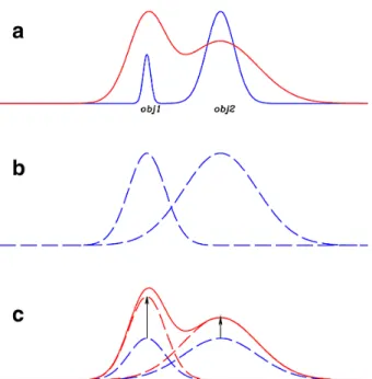
is outlined in the flowchart given in Fig.2. The following paragraphs give a short description of the pipeline.

Fig. 1.Schematic representation of the PSF-matched algorithm imple-mented in

_{-}

. Top: two objects are clearly detected and separated in the high-resolution detection image (blue line). The same two objects are blended in the low-resolution measurement image and have different colours (red line). Middle: the two objects are isolated in the detection image and are individually smoothed to the PSF of the measurement image, to obtain normalized model templates. Bottom: the intensity of each object is scaled to match the global profile of the measurement im-age. The scaling factors are found with a global χ2_{minimization over}

the object areas. Image fromDe Santis et al.(2007).

2.1.1. Input

The input files needed by

_{-}

vary depending on the type(s) of priors used.

If true high-resolution priors are used, e.g. for optical/NIR ground-based or IRAC measurements using HST cutouts,

-

needs

– the detection, high-resolution image (HRI) in .fits format; – the catalogue of the sources in the HRI, obtained using SE

_{}

or similar codes (the required format is de-scribed in Appendix A);

– the segmentation map of the HRI, in .fits format, again obtained using SE

_{}

or similar codes, having the value of the id of each source in the pixels belonging to it, and zero everywhere else;

– a convolution kernel K, in the format of a .fits image or of a .txt file, matching the PSFs of the HRI and the LRI so that PS FLRI= K ∗PS FHRI(∗ is the symbol for convolution).

The kernel must have the HRI pixel scale.

If analytical models are used as priors (e.g. G

_{}

models),

-

needs

– the stamps of the models (one per object, in .fits format); – the catalogue of the models (the required format is described

in Appendix A);

– the convolution kernel K matching the PSFs of the HRI and the LRI, as in the previous case.

If models have more than one component, one separate stamp per component and catalogues for each component are needed (e.g. one catalogue for bulges and one catalogue for disks).

If unresolved, point-like priors are used,

_{-}

needs – the catalogue of positions (the required format is described

in Appendix A);

– the LRI PSF, in the LRI pixel scale.

In this case, a potential limitation to the reliability of the method is given by the fact that the prior density usually needs to be optimized with respect to FIR/sub-mm maps, as discussed in Shu et al. (in prep.) andElbaz et al. (2011) (see also Wang et al.; Bourne et al., in prep.). The optimal number of priors turns out to be around 50–75% of the numbers of beams in the map. The main problem is identifying which of the many potential priors from, for example, an HST catalogue one should use. This is a very complex issue and we do not discuss it in this paper.

If mixed priors are used,

_{-}

obviously needs the input files corresponding to each of the different types of priors in use.

Finally, in all cases

_{-}

needs

– the measure LRI, background subtracted (see next para-graph), in .fits format, with the same orientation as the HRI (i.e. no rotation allowed); the pixel scale can be equal to, or an integer multiple of, the HRI pixel scale, and the origin of one pixel must coincide; it should be in surface brightness units (e.g. counts/s/pixel, or Jy/pixel for FIR images, and not PSF-filtered);

– the LRI rms map, in .fits format, with the same dimen-sions and WCS of the LRI.

Table 1 summarizes the input requirements for the different choices of priors just described.

All the input images must have the following keywords in their headers: CRPIXn, CRVALn, CDn_n, CTYPEn (n= 1, 2). 2.1.2. Background subtraction

As already mentioned, the LRI must be background subtracted before being fed to

_{-}

. This is of particular interest when dealing with FIR/sub-mm images, where the typical standard is to use zero-mean. To estimate the background level in opti-cal/NIR images, one simple possibility is to take advantage of the option to fit point-like sources to measure the flux for a list of positions chosen to fall within void regions. The issue is more problematic in such confusion-limited FIR images where there are no empty sky regions. In such cases, it is important to sep-arate the fitted sources (those listed in the prior catalogue) from the background sources, which contribute to a flat background level behind the sources of interest. The priors should be cho-sen so that these two populations are uncorrelated. The average contribution of the faint background source population can then be estimated for example by i) injecting fake sources into the map and measuring the average offset (output-input) flux; or ii) measuring the modal value in the residual image after a first pass through

_{-}

(see e.g. Bourne et al., in prep.).

2.1.3. Stages

-

goes through “stages”, each of which performs a well-defined task. The best results are obtained by performing two runs (“pass 1” and “pass 2”), the second using locally regis-tered kernels produced during the first. The possible stages are the following:

– priors: creates/organizes stamps for sources as listed in the input priors catalogue(s);

Fig. 2.Schematic representation of the workflow in

_{-}

.

Table 1. Input files needed by

-

for different settings (see text for details).

Real cutouts Analytical models Point-sources Priors HRI Segmentation Catalogue HRI Model Stamps Catalogue Positions Catalogue Transformation Convolution Kernel Convolution Kernel PSFLRI

Measure LRI rmsLRI LRI rmsLRI LRI rmsLRI

– convolve: convolves each high-resolution stamp with the convolution kernel K to obtain models (“templates”) of the sources at LRI resolution. The templates are normalized to unit total flux. If the pixel scale of the images is different, transforms templates accordingly. Convolution is preferably performed in Fourier space, using fast FFTW3 libraries; how-ever the user can choose to perform it in real pixel space, ensuring a more accurate result at the expense of a much slower computation.

– positions: if an input catalogue of unresolved sources is given, creates the PSF-shaped templates listed in it, and merges it with the one produced in the convolve stage; – fit: performs the fitting procedure, solving the linear

sys-tem and obtaining the multiplicative factors to match each template flux with the measured one;

– diags: selects the best fits2 and produces the final format-ted output catalogues with fluxes and errors, plus some other diagnostics, see Sect.2.3;

2 _{Each source is fitted more than once if an arbitrary grid is used, as in}

the standard

_

approach.

– dance: obtains local convolution kernels for the second pass; it can be skipped if the user is only interested in a single-pass run;

– plotdance: plots diagnostics for the dance stage; it can be skipped for any purpose other than diagnostics;

– archive: archives all results in a subdirectory whose name is based on the LRI and the chosen fitting method (to be used only at the end of the second pass).

The exact pipeline followed by the code is specified by a key-word in the input parameter file. See also Appendix A for a more detailed description of the whole procedure.

2.1.4. Solution of the linear system

The search for the LRI fluxes of the objects detected in the HRI is performed by creating a linear system

X m, n I(m, n)=X m, n N X i FiPi(m, n) (1)

where m and n are the pixel indexes, I contains the pixel values of the fluxes in the LRI, Piis the normalized flux of the template

for the ith objects in the (region of the) LRI being fitted, and Fi

is the multiplicative scaling factor for each object. In physical terms, Firepresents the flux of each object in the LRI (i.e. it is

the unknown to be determined).

Once the normalized templates for each object in the LRI (or region of interest within the LRI) have been generated during the convolve stage, the best fit to their fluxes can be simultaneously derived by minimizing a χ2statistic,

χ2₌ " P m, nI(m, n) − M(m, n) σ(m, n) #2 (2) where m and n are the pixel indexes,

M(m, n)=

N

X

i

FiPi(m, n) (3)

and σ is the value of the rms map at the (m, n) pixel position. The output quantities are the best-fit solutions of the mini-mization procedure, i.e. the Fiparameters and their relative

er-rors. They can be obtained by resolving the linear system ∂χ2

∂Fi

= 0 (4)

for i= 0, 1, ..., N.

In practice, the linear system can be rearranged into a matrix equation,

AF= B (5)

where the matrix A contains the coefficients PiPj/σ2, F is a

vec-tor containing the fluxes to be determined, and B is a vecvec-tor given by IiPi/σ2 terms. The matrix equation is solved via one

of three possible methods as described in the next subsection.

2.1.5. Fitting options

-

allows for some different options to perform the fit: – three different methods for solving the linear system are

im-plemented, namely, the LU method (used by default in

_

), the Cholesky method, and the Iterative Biconjugate Gradient method (used by default in

_{}

; for a review on meth-ods to solve sparse linear systems see e.g.Davis 2006). They yield similar results, although the LU method is slightly more stable and faster;

– a threshold can be imposed so that only pixels with a flux higher than this level will be used in the fitting procedure (see Sect.4.1.4);

– sources fitted with a large, unphysical negative flux ( fmeas <

−3σ, where σ is their nominal error, see below) can be ex-cluded from the fit, and in this case a new fitting loop will be performed without considering these sources.

The fit can be performed i) on the entire LRI as a whole, pro-ducing a single matrix containing all the sources (this is the method adopted in

_{}

); ii) subdividing the LRI into an arbitrary grid of (overlapping) small cells, perfoming the fit in each of such cells separately, and then choosing the best fit for each source, using some convenient criteria to select it (because sources will be fitted more than once if the cells overlap; this is the method adopted in

_

); iii) ordering objects by decreasing

flux, building a cell around each source including all its poten-tial contaminants, solving the problem in that cell and assigning to the source the obtained flux (cells-on-objects method; see the Appendix for more details).

While the first method is the safest and more accurate be-cause it does not introduce any bias or arbitrary modifications, it may often be unfeasible to process at once large or very crowded images. Potentially large computational time saving is possible using the cells-on-objects method, depending on the level of blending/confusion in the LRI; if it is very high, most sources will overlap and the cells will end up being very large. This ul-timately results in repeating many times the fit on regions with dimensions comparable to the whole image (a check is imple-mented in the code, to automatically change the method from cells-on-objectsto single fit if this is the case). If the confusion is not dramatic, a saving in computational time up to two orders of magnitude can be achieved. The results obtained using the cells-on-objectsmethod prove to be virtually identical to those obtained with a single fit on the whole image (see Sect.4.1.2). On the other hand, using the arbitrary cells method is normally the fastest option, but can introduce potentially large errors to the flux estimates owing to wrong assignments of peripheral flux from sources located outside a given cell to sources within the cell (again, see Sect.4.1.2and the Appendix B).

2.1.6. Post-fitting stages: kernel registration

After the fitting procedure is completed,

_{-}

will produce the final output catalogues and diagnostic images (see Sect.2.3). Among these, a model image is obtained by adding all the tem-plates, scaled to their correct total flux after fitting, in the po-sitions of the sources. This image will subsequently be used if a second pass is planned; during a stage named dance, a list of positional shifts is computed, and a set of shifted kernels are gen-erated and stored. The dance stage consists of three conceptual steps:

– the LRI is divided into cells of a given size (specified by the keyword dzonesize) and a linear∆x, ∆y shift is computed within each cell, cross-correlating the model image and the LRI in the considered region3;

– interpolated shifts are computed for the regions where the previous registration process gives spuriously large shifts, i.e. above the given input threshold parameter maxshift; – the new set of kernels is created using the computed shifts to

linearly interpolate their positions, while catalogues report-ing the shifts and the paths to kernels are produced.

2.1.7. Second pass

The registered kernels can subsequently be used in the second pass run to obtain more astrometrically precise results.

_{-}

automatically deals with them provided the correct keyword is given in the parameter file. If unresolved priors are used, the list of shifts generated in the dance stage will be used by the positions routine during the second pass to produce correctly shifted PSFs and generate new templates.

3 _{FFT and direct cross-correlations are implemented, the latter being}

the preferred default choice because it gives more precise results at the expense of a slightly slower computation.

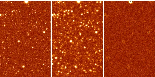
Fig. 3. Example of the results of a standard

-

run using extended priors. Left to right: HRI (FW H M = 0.200

), LRI (FW H M = 1.6600

), and residuals image for a simulated dataset. LRI and residual image are on the same greyscale.

2.2. Error budget

During the fitting stage, the covariance matrix is constructed. Errors for each source are assigned as the square root of the di-agonal element of the covariance matrix relative to that source. It must be pointed out that using any cell method for the fitting rather than the single fitting option will affect this uncertainty budget, since a different matrix will be constructed and resolved in each cell.

It is important to stress that this covariance error budget is a statistical uncertainty, relative to the rms fluctuations in the measurement image, and is not related to any possible systematic error. The latter can instead be estimated by flagging potentially problematic sources, to be identified separately from the fitting procedure. There can be different possible causes for systematic offsets of the measured flux with respect to the true flux of a source.

_{-}

assigns the following flags:

– +1 if the prior has saturated or negative flux;

– +2 if the prior is blended (the check is performed on the segmentation map);

– +4 if the source is at the border of the image (i.e. its segmen-tation reaches the limits of the HRI pixels range).

2.3. Description of the output

-

output files are designed to be very similar in format to those produced by

_

. They provide

– a “best” catalogue containing the following data, listed for each detected source (as reported in the catalogue file header):

– id;

– x and y positions (in LRI pixel scale and reference frame, FITS convention where the first pixel is centred at 1,1); – id of the cell in which the best fit has been obtained (only

relevant for the arbitrary grid fitting method);

– x and y positions of the object in the cell and distance from the centre (always equal to 0 if the cells-on-objects method is adopted);

– fitted flux and its uncertainty (square root of the variance, from the covariance matrix). These are the most impor-tant output quantities;

– flux of the object as given in the input HRI catalogue or, in the case of point-source priors, measured flux of the pixel at the x, y position of the source in the LRI; – flux of the object as determined in the cutout stage

(it can be different to the previous one, e.g. if the

segmentation was dilated); in the case of point-sources priors, measured flux of the pixel at the x, y position of the source in the LRI;

– flag indicating a possible bad source as described in the previous subsection;

– number of fits for the object (only relevant for arbitrary grid fitting method, 1 in all other cases).

– id of the object having the largest covariance with the present source;

– covariance index, i.e. the ratio of the maximum covari-ance to the varicovari-ance of the object itself; this number can be considered an indicator of the reliability of the fit, since large covariances often indicate a possible system-atic offset in the measured flux of the covarying objects (see Sect.4.1.2).

– two catalogues reporting statistics for the fitting cells and the covariance matrices (they are described in the documentation);

– the model .fits image, obtained as a collage of the tem-plates, as already described;

– a diagnostic residual .fits image, obtained by subtracting the model image from the LRI;

– a subdirectory containing all the low-resolution model templates;

– a subdirectory containing the covariance matrices in graphic (.fits) format;

– a few ancillary files relating to the shifts of the kernel for the second pass and a subdirectory containing the shifted kernels.

All fluxes and errors are output in units consistent with the input images.

Figures3–5show three examples of

_{-}

applications on simulated and real data, using the three different options for priors.

3. Assumptions and limitations

The PSF-matching algorithms implemented in

_{-}

and de-scribed in the previous section are prone to some assump-tions and limitaassump-tions. In particular, the following issues must be pointed out.

i) The accuracy of the results strongly depends on the reliabil-ity of the determined PSFs (and consequently of the convo-lution kernel). An error of a few percentage points in the central slope of the PSF light profile might lead to non-negligible systematical deviations in the measured fluxes.

Fig. 4. Example of the results of a standard

-

run using point-source priors. Left to right: LRI (FW H M = 2500

) and residuals im-age (same greyscale) for a simulated dataset. See also Sect.4.1.2.

Fig. 5. Example of the results of a standard

-

run using analytical priors. Left to right: CANDELS COSMOS H-band (HRI), R-band (LRI) and residuals image obtained us-ing G



two-component models. LRI and residual image are on the same greyscale.

Fig. 6.Typical patterns in a residual image created by

_{-}

, caused by inaccurate PSF/kernel determination. In this case, the ring-shaped shadow surrounding a bright central spot is due to an underestimation of the central peak of the LRI PSF, which causes an overestimation of the fit in the outskirts while leaving too much light in the centre.

However, since the fitting algorithm minimizes the residu-als on the basis of a summation over pixels, an incorrect PSF profile will lead to characteristic positive and negative ring-shaped patterns in the residuals (see Fig. 6), and to some extent the summation over pixels will compensate the global flux determination.

ii) When dealing with extended priors, it is assumed that the instrinsic morphology of the objects does not change with the wavelength. Of course, this is usually not the case. The issue is less of a problem when dealing with FIR images, in which the morphological features of the priors are unre-solved by the low-resolution PSF. On the other hand, in the optical and NIR domains this problem may be solved by the

use of multicomponent analytical models as priors. In this approach, each component should be fitted independently, thus allowing the ratio between bulge and disk components to vary between the HRI and LRI. A clear drawback of this approach is that any failure of the fit due to irregular or dif-ficult morphological features (spiral arms, blobs, asymme-tries, etc.) would be propagated into the LRI solution. This functionality is already implemented in

_{-}

and detailed testing is ongoing.

iii) As explained in Sect.2.2,

_{-}

flags priors that are likely to be flawed: sources too close to the borders of the image, saturated objects, and most notably blended priors. The as-sumption that all priors are well separated from one another is crucial, and the method fails when this requirement is not accomplished. Again, this is crucial only when dealing with real priors, while analytical models and unresolved priors are not affected by this limitation.

iv) As anticipated in Sect.2.1.1, FIR images can suffer from an “overfitting” problem, due to the presence of too many priors in each LRI beam if the HRI is deeper than the LRI. In this case, a selection of the priors based on some additional crite-ria (e.g. flux predition from SED fitting) might be necessary to avoid catastrophic outcomes (see also Wang et al.; Bourne et al., in prep.).

4. Validation

To assess the performance of

_{-}

we set up an extensive set of simulations, aimed at various different and complementary goals.

We used S

_

M

_

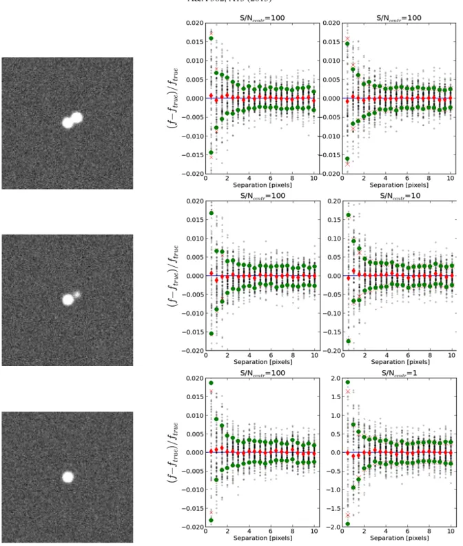
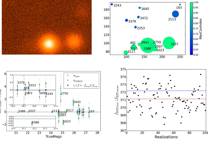
(Bertin 2009), a public software tool, to build synthetic .fits images. The code ensures direct control

Fig. 7.Accuracy check on idealized PSF-shaped objects. 100 realizations of the same image containing two PSF-shaped objects at varying positions and signal-to-noise ratios have been produced and the fluxes have been measured with

_{-}

. In each row, the left image shows one of the 100 realizations with the largest considered separation (10 pixels). On the right, the first panel refers to the central object, and the second (on the right) to the shifted object; central signal-to-noise (S/Ncentr) ratios are, from top to bottom, 100, 100, 100 for the first source and 100, 10, 1 for

the second source. In each panel, as a function of the separation interval between the two sources, the faint grey points show each of the 100 flux measurements (in relative difference with respect to the true input flux), the red diamonds are the averages of the 100 measurements, the red crosses show the nominal error given by the covariance matrix in

_{-}

, and the green dots the standard deviation of the 100 measurements. See text for more details.

on all the observational parameters (the magnitude and positions of the objects, their morphology, the zero point magnitude, the noise level, and the PSF). Model galaxies were built by summing a de Vaucouleurs and an exponential light profile in order to best mimic a realistic distribution of galaxy morphologies. These models were generated using a variety of bulge-to-total light ra-tios, component sizes, and projection angles.

All tests were run using ideal (i.e. synthetic and symmetric) PSFs and kernels.

Moreover, we also performed tests on real datasets taken from the CANDELS survey (in these cases using real PSFs).

Some of the tests were performed using both

_{-}

and



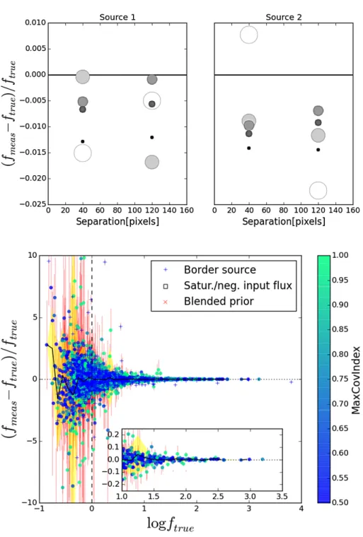
, to cross-check the results, ensuring the perfect equiva-lency of the results given by the two codes when used with the

Fig. 8.Effects of different segmentation areas

on the measured flux of two isolated objects with identical flux and signal-to-noise ratio, at two possible separations of 40 and 120 pixels. Each panel shows the flux error in one of the objects at each separation distance. The shades and dimensions of the dots is a function of the radius of the segmentation, with darker and smaller dots corresponding to smaller segmen-tations. See text for more details.

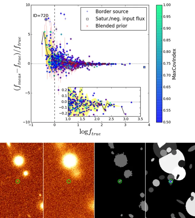
Fig. 9. Accuracy of the flux determination in a simulation containing non-overlapping, PSF-shaped sources and “perfect” detection. Relative measured flux difference ( fmeas −

ftrue)/ ftrueis plotted versus logarithm of the

in-put flux ftrue, for a simulated image populated

with PSF-shaped sources (FW H M = 1.6600

). Each dot corresponds to a single source, with different symbols and colours referring to vari-ous diagnostics as explained in the legend and in the colourbar. The black solid line is the aver-age in bins, the yellow shade is the standard de-viation. The vertical dashed line shows the lim-iting flux at 1σ, f = 1. The inner panel shows a magnification of the brighter end of the dis-tribution. The fit was performed on the whole image at once. See text for more details.

same parameter sets, and showing how appropriate settings of the

_{-}

parameters can ensure remarkable improvements.

For simplicity, here we only show the results from a re-stricted selection of the test dataset, which are representative of the performance of

_{-}

in standard situations. The results of the other simulations resemble overall the ones we present, and are omitted for the sake of conciseness.

4.1. Code performance and reliability on simulated images 4.1.1. Basic tests

As a first test, we checked the performance of the basic method by measuring the flux of two PSF-shaped synthetic sources, with varying separation and signal-to-noise ratios. One hun-dred realizations with different noise maps of each parameter set were prepared, and the averages on the measured fluxes were

computed. The aims of this test were twofold: on the one hand, to check the precision to which the fitting method can retrieve true fluxes in the simplest possible case - two sources with ideal PSF shape; on the other hand, to check the reliability of the nom-inal error budget given by the covariance matrix, comparing it to the real rms of the 100 measurements. Figure7shows three ex-amples of the set-up and the results of this test. Clearly, in both aspects the results are reassuring: the average of the 100 mea-surements (red diamonds) is always in very good agreement with the true value, with offset in relative error always well under the 1/(S/N)centrlimit ((S/N)centris the value of the signal-to-noise

ra-tio in the central pixel of the source, corresponding to roughly one third of the total S/N); and the nominal error (red crosses) given by the covariance matrix is always in good agreement with the rms of the 100 measurements (red circles).

When dealing with extended objects rather than with point-like sources, one must consider the additional problem that the

Fig. 10.Analysis of a small region including a strongly covarying group of sources. Upper left panel: one of the 100 realizations with different noise maps of the region. Upper right panel: true spatial position of all the sources in the region (the colour of the dots refer to the covariance index of the sources, as indicated in the colourbar, while their size is proportional to their true flux). Bottom left panel: relative deviation of measured flux from the true flux for each source in the region, as a function of their true magnitude (big dots show the average relative deviation, and their colours refer to their covariance index as in the previous panel; green squares show the nominal uncertainty given by

_{-}

, to be compared with the rms of the distribution of the 100 measurements (diamonds); small grey dots are the 100 measurements. The insets show magnifications of regions of interest). Bottom right panel: each dot shows the sum of the measured fluxes for each of the 100 realizations, and the average of this sum (red line) to be compared with the true sum (blue line), showing that an overall consistency is guaranteed by the method. See text for more details.

entire profile of the source cannot be measured exactly be-cause the segmentation is limited by the lowest signal-to-noise isophote. The extension of the segmentation therefore plays a crucial role and defining it correctly is a very subtle problem. Simply taking the isophotal area as reported by SE

_{}

as ISOAREA often underestimates the real extension of the ob-jects. Accordingly, the segmentation of the sources should some-how be enlarged to include the faint wings of sources. To this aim, specific software called D

_{}

was developed at OAR and used in the CANDELS pipeline for the photometric analysis of GOODS-S and UDS IRAC data (Galametz et al. 2013). D

_{}

enlarges the segmentation by a given factor, depending on the original area; it has proven to be reasonably robust in minimiz-ing the effects of underestimated segmentated areas.

Figure8shows the effects of artificially varying the dimen-sions of the segmentation relative to two bright, extended and isolated sources in a simulated HRI, on the flux measured for that source in a companion simulated LRI. It is important to note how enlarging the segmented area normally results in larger measured fluxes, because more and more light from the faint wings of the source are included in the fit. However, beyond a certain limit the measurements begin to lose accuracy owing to the inclusion of noisy, too low signal-to-noise regions (which may cause a lower flux measurement).

In principle, using extended analytical models rather than real high-resolution cutouts should cure this problem more e ffi-ciently, because models have extended wings that are not signal-to-noise limited. Tests are ongoing to check the performance of this approach, and will be presented in a forthcoming paper.

4.1.2. Tests on realistic simulations

The next tests were aimed at investigating less idealized sit-uations, and have been designed to provide a robust analysis of the performance of the code on realistic datasets. We used the code G

_

C

_

(Schreiber et al., in prep.) to produce mock catalogues of synthetic extragalactic sources, with reasonable morphological features and flux distribution4_{. Then, a set of} images were produced using such catalogues as an input for

4 _G



C

_

is another software package developed within the

-

project. It uses GOODS-S CANDELS statistics to generate a realistic distribution of masses at all redshifts, for two populations of galaxies (active and passive), consistently with observed mass func-tions. All the other physical properties of the mock galaxies are then estimated using analytical recipes from literature: each source is as-signed a morphology (bulge-to-total ratio, disk and bulge scale lengths, inclination etc.), star formation rate, attenuation, optical and infrared rest-frame, and observed magnitudes. Each source is finally assigned a

Fig. 11.Accuracy of the flux determination in a simulation containing extended objects, overlapping priors, and SE



detection. Top: relative flux difference ( fmeas− ftrue)/ ftrueversus logarithm of the input flux ftruefor a simulated image populated with extended sources (FW H M=

1.6600

). Symbols and colours are as in Fig.9. The inner panel shows a magnification of the brighter end of the distribution. The outlier marked with the open black circle, ID= 720, is shown in the bottom panel: left to right, HRI (FWHM = 0.200_{), LRI, SE}



segmentation map and “true” segmentation map. The green circles show the object detected via SE

_{}

, while the blue cross shows its “true” position. See text for more details.

S

_

M

_

. A “detection” HRI mimicking an HST H-band ob-servation (FW H M = 0.200) was generated from the G

_

C

_

catalogue using output parameters to characterize the objects’ extended properties. Then a set of measure LRIs were pro-duced: the first was populated with PSF-shaped sources, having FW H M = 1.6600 _{(the typical IRAC-ch1/ch2 resolution, a key}

application for

_{-}

), while other LRIs were created from the input catalogue, mimicking different ground-based or IRAC full

sky-projected position mimicking the clustering properties of the real CANDELS data.

width at half maxima (FWHMs). Finally, we created another HRI catalogue removing all of the overlapping sources5. This “non-overlapping” catalogue was used to create parallel detec-tion and measurement images in order to obtain insight into the complications given by the presence of overlapping priors. In

5 _{We proceeded as follows. First, we created a “true” segmentation}

image using the input catalogue and assigning to each object all the pixels in which the flux was 1.005 × fbackground. Then, starting from the

beginning of the list, we included each source in the new catalogue if its segmented area did not overlap the segmented area of another already inserted source.

Fig. 12.Accuracy of the flux determination in a FIR-like simulation (Herschel SPIRE 250 µm, FW H M = 2500

, 3.600

pixel scale), using un-resolved priors. The symbols have the same meaning as in Fig.11. See text for more details.

all these images, the limiting magnitude was set equal to the as-signed zero point, so that the limiting flux at 1σ is 1. In addition, the fits were always performed on the LRI as a whole, if not otherwise specified.

Figure9shows the results relative to the first test, i.e. the fit on the image containing non-overlapping, PSF-shaped sources, with a “perfect” detection (i.e. the priors catalogue contains all sources above the detection limit), obtained with a single fit on the whole image. The figure shows the relative error in the mea-sured flux of the sources, ( fmeas − ftrue)/ ftrue, versus the log of

the real input flux ftrue; the different symbols refer to the flag

assigned to each object, while the colour is a proxy for the co-variance index.

In this case, the only source of uncertainty in the measure-ment is given by the noise fluctuations, which clearly become dominant at the faint end of the distribution. Looking at the er-ror bars of the sources, which are given by the nominal erer-ror assigned by

_{-}

from the covariance matrix, one can see that almost all sources have measured flux within 2σ from their true flux, with only strongly covariant sources (covariance index '1, greener colours) having | fmeas− ftrue|/ ftrue> 1σ. The only

notice-able exceptions are sources that have been flagged as potentially unreliable, as described in Sect.2.2. We also note how the av-erage ∆ f / f (solid black line) is consistent with zero down to

ftrue= S/N ' 0.63.

Figure10 shows the analysis of a case study in which the fluxes of a clump of highly covariant objects are measured with poor accuracy, and some of the nominal uncertainties are under-estimated: a very bright source (ID 3386, mtrue= 21.17) shows a

relative difference ( fmeas− ftrue)/ ftrue > 3σ. To cast light on the

reason for such a discrepancy, the region surrounding the object was replicated 100 times with different noise realizations, and the results were analysed and compared. The upper panels show (left) one of the 100 measurement images and (right) the position of all the sources in the region (many of which are close to the detection limit). The colour code refers to the covariance index of the sources. The bottom left panel shows the relative error in the measured flux for all the sources in the region, with the in-ner panels showing magnifications relative to the object ID 3386

and to the bunch of objects with mtrue ∼ 26.5. Looking at the

colours of their symbols, many objects in the region turn out to be strongly covariant. Indeed, while the bluer sources in the up-per part of the region all have covariant indexes lower than 0.5, the greener ones in the crowded lower part all have covariance index larger than 1 (indeed larger than 2 in many cases). This means that their flux measurements are subject to uncertainties not only from noise fluctuations, but also from systematic errors due to their extremely close and bright neighbours. As clearly demonstrated here, the covariance index can give a clue to which measurements can be safely trusted.

The bottom right panel gives the sum of the measured fluxes of all sources in each of the 100 realizations (the blue line is the true total flux and the red line is the mean of the 100 measured total fluxes). It can be seen that the total flux measured in the region is always consistent with the expected true one to within '1% of its value.

Although it is not possible to postulate a one-to-one rela-tion (because in most cases sources having a large covariance index have a relatively good flux estimate, see Fig.9), the bot-tom line of this analysis is that the covariance index, together with the flagging code outputted by

_{-}

, can give clues about the reliability of measured flux, and should be taken into consid-eration during the analysis of the data. Measurements relative to sources having a covariance index larger than 1 should be treated with caution.

In a subsequent more realistic test, we considered extended objects (including morphologies of objects from the G

_

C

_

catalogue, using FW H MHRI = 0.200 and FW H MLRI = 1.6600

and imposing mtrue,LRI = mtrue,HRI = mH160,GenCat for

simplic-ity) and allowed for overlapping priors. To be consistent with the standard procedure adopted for real images, for this case we proceeded by producing an SE

_{}

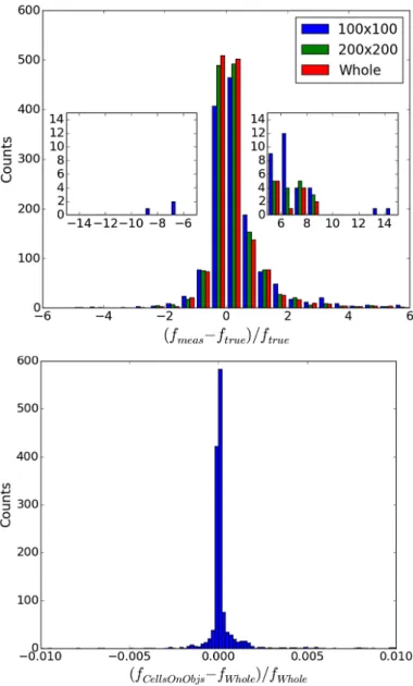
catalogue and seg-mentation map, which were then spatially cross-correlated with the “true” input catalogue. The results for this test are shown in Fig.11. Even in this much more complex situation, the re-sults are reassuring; there is an overall good agreement between measured and input fluxes for bright (log S/N > 1) sources, with only a few flagged objects clearly showing large deviations

Fig. 13.Accuracy of the flux determination. Top panel: for the same simulation described in Fig. 11, the histograms show the results for three different fitting methods: regular grid 100 × 100 pixels (standard



approach), regular grid 200 × 200, single fit on the whole image. The small boxes show the extended wings of the histograms, magnified for better viewing. The accuracy increases by enlarging the cells and, reaches the best result with the single fit on the whole image. Bottom panel: the histogram shows the relative measured flux difference be-tween the single fit on the whole image and the cells-on-objects method. Differences above 1% are very rare.

from the expected value, and a reasonably good average agree-ment down to log S/N = 0. However, all bright fluxes are mea-sured '5% fainter than the true values (see the inner box in the same figure); this is very likely the effect of the limited segmen-tation extension, as already discussed in the previous section. On the other hand, faint sources tend to have systematically overestimated fluxes, arguably because of contamination from undetected sources. To confirm this, we focus our attention on a single case study (the source marked as ID 720) which shows a large discrepancy from its true flux, but has a relatively small co-variance index. An analysis of the real segmentation map shows how the detected object is actually a superposition of two differ-ent sources that have been detected as a single one, so that the measured flux is of course higher than expected. One should also

note that the uncertainties on the measured fluxes are smaller in this test, because there are fewer priors (only the ones detected by SE

_{}

are now present), implying a lower rank of the covariance matrix and a lower number of detected neighbours blending in the LRI. This causes a global underestimation of the errors.

To check the performance of

_{-}

at FIR wavelengths, we also run a test on a simulated Herschel SPIRE 250 µm im-age (FW H M = 2500, 3.600 pixel scale). The simulated image (shown alongside with the obtained residuals in Fig.4) mim-ics real images from the GOODS-Herschel program, the deep-est Herschel images ever obtained. This image was produced with the technique presented in Leiton et al. (2015); we first derived (predicted) flux densities for all the 24 µm detections

(F24 µm > 20 µJy) in GOODS-North, which are dependent

on their redshift and flux densities at shorter wavelengths, and then we injected these sources into the real noise maps from GOODS-Herschel imaging. Additional positional uncertainties, typically 0.500, were also applied to mimic real images. As shown

inLeiton et al.(2015), these simulated images have similar pixel

value distributions to real images (see also Wang et al., in prep., for more details). For this test,

_{-}

was run using the list of all the 24 µm sources as unresolved priors. The results of the test are plotted in Fig.12, and they show that even in this case

-

can recover the input fluxes of the sources with great statistical accuracy (the mean of the relative deviation from the expected measurements, i.e. the black solid line in the plot, is consistent with zero down to the faintest fluxes). The results are equivalent to those obtained on the same datasets with other pub-lic software specifically developed for FIR photometry, such as

F

_

P

_

(Béthermin et al. 2010).

4.1.3. Testing different fitting options: cell dimensions We then proceeded to check the performance of the different fitting techniques that can be used in

_{-}

. To this aim, we repeated the test on the 1.6600 LRI with extended priors and SE

_{}

priors, described in Sect. 4.1.2, with different fitting methods: using a regular grid of cells of 100 × 100 pixels, a regular grid of cells of 200 × 200 pixels, and the cells-on-objects method, comparing the results with those from the fit of the whole image at once. The results of the tests are shown in Figs.13and14. The first figure compares the distributions of the relative errors in measured flux for the runs performed on the 100 × 100 pixels grid, on the 200 × 200 pixels grid, and on the whole image at once. Clearly, using any regular grid of cells worsens the results, as anticipated in Sect.2.1.5. Enlarging the sizes of the cells improves the situation, but does not completely solve the problem. We note that the adoption of an arbitary grid of cells of any dimension in principle is prone to the introduction of potentially large errors, because (possibly bright) contaminating objects may contribute to the brightness measured in the cell, without being included as con-tributing sources. A mathematical sketch of this issue is ex-plained in the Appendix B (see also Sect.4.2). The second his-togram compares the differences between the fit on the whole image and the fit with the cells-on-objects method. Almost all the sources yield identical results with the two methods, within ( fmeas− ftrue)/ ftrue< 0.001, which proves that the cells-on-objects

method can be considered a reliable alternative to the single-fit method. Finally, Fig. 14 compares the HRI, the LRI, and the residual images obtained with the four methods and their distri-butions of relative errors, showing quantitatively the difference between the analyzed cases.

Fig. 14.Accuracy of the flux determination. For the same simulation described in Fig.11, the plots show the results for four different fitting methods. Top panel, left to right: HRI (FW H M= 0.200

), LRI (FW H M= 1.6600

), residuals using a regular grid of 100 × 100 pixels cells (standard



approach), a regular grid of 200 × 200 pixels cells, a single fit on the whole image, and the cells-on-objects method. The spurious fluctuations in the last two panels are due to segmentation inaccuracies, as in Fig.11. Bottom panels, left to right and top to bottom: relative measured flux differences with respect to true fluxes, same order as above. The values of the covariance index are different in each case because of the varying sizes of the cells (and therefore of the relative matrix).

In summary, it is clear that an incautious choice of cell size may lead to unsatisfactory and catastrophic outcomes. On the other hand, the advantages of using a single fit, and the equivalence of the results obtained with the single-fit and the cells-on-objectstechniques, are evident. As already anticipated, one should bear in mind that the cells-on-objects method is only convenient if the overlapping of sources is not dramatic, as in ground-based optical observations. For IRAC and FIR images, on the other hand, the extreme blending of sources would cause the cells to be extended over regions approaching the size of the whole image, so that a single fit would be more convenient, al-though often still CPU-time consuming.

4.1.4. Testing different fitting options: threshold fitting

As described in Sect.2.1.5,

_{-}

includes the option of impos-ing a lower threshold on the normalized fluxes of templates so as to exclude low signal-to-noise pixels from the fit. Figure 15

shows a comparison of the relative errors obtained with three different values of the THRESHOLD parameter: t = 0, t = 0.5, and t = 0.9 (whic means that only pixels with normalized flux

fnorm > t × fpeakin the convolved template will be used in the

fitting procedure). The differences are quite small; however, a non-negligible global effect can be noticed: all sources tend to slightly decrease their measurement of flux when using a thresh-old limit. This brings faint sources (generally overestimated without using the threshold) closer to their true value, at the same time making bright sources too faint. This effect deserves care-ful investigation, which is beyond the scope of this study, and is postponed to a future paper.

4.1.5. Colours

A final test was run introducing realistic colours, i.e. assign-ing fluxes to the sources in the LRI consistent with a realistic SED (as output by G

_{C}

, see Sect.4.1.2), instead of impos-ing them to be equal to the HRI fluxes. We took IRAC-ch1 as a reference filter for the LRI, consistently with the chosen FWHM of 1.6600_{. Furthermore, we allowed for variations in the}

bulge-to-disc ratios of the sources to take possible effects of colour gradients into account. We compared the results obtained with

Fig. 15. Effects of threshold fitting (Sect. 4.1.4). Mean relative error (black line) and standard devia-tion (yellow shaded area) for three simuladevia-tions with different threshold values (0.0, 0.5, 0.9). Only pix-els with normalized flux higher than the threshold values are included in the fit. Larger threshold val-ues result in more accurate measurements for faint sources, at the expense of a systematic underesti-mation of the flux for brighter ones.

Fig. 16.Top: measured magnitude differences (mmeas−

mtrue) versus “true” input magnitudes mtrue, for two

sim-ulated images popsim-ulated with extended sources (HRI has FW H M = 0.200

and HST H-band-like fluxes, LRI has FW H M = 1.6600 _{and IRACch1-like fluxes),}

us-ing three different methods: SEdual-mode aperture, SE

_{}

dual-mode “best”, and

_{-}

. Vertical lines show the 5σ (dashed) and 1σ (dotted) limits of the simulated LRI. Bottom: magnification of the top panel, showing only

_{-}

results, colour-coded as a function of the covariance index. See text for more details.

determine the magnitudes of the sources in the LRI: namely, SE

_{}

dual mode aperture and MAG_BEST photometry (with HRI as detection image). The differences between mea-sured and input magnitudes in the LRI, mmeas–mtrue, are plotted

in Fig.16. Clearly,

_{-}

ensures the best results, with much less scatter in the measurements than both of the other two meth-ods, and very few outliers.

4.2. Performance on real datasets

It is instructive to check how

_{-}

performs on real datasets, in addition to simulations. To this aim, we run two different tests. In the first, we compared the results of the

_

CANDELS anal-ysis on the UDS CANDELS I-band (Galametz et al. 2013) to a

_{-}

run obtained using the cells-on-objects method and different parameters in the kernel registration stage. Figure 17

shows the histograms of the differences in the photometric mea-surements between

_

and

_{-}

. Many sources end up with a substantially different flux, because of the two cited factors (a better kernel registration and the different fitting procedure). We note that the majority of the sources have fainter fluxes with respect to the previous measurements, precisely because of the effect described in Sect.4.1.2: fitting using a grid of cells

Fig. 17.UDS I-band



versus

-

comparison. Top panel: com-pared measured fluxes. Bottom panel: histogram of relative measured flux difference.

Fig. 18. UDS I-band

_

versus

_{-}

comparison. The panels on the left show two small patches of the official CANDELS residual image obtained using

-

. The residual images of the same regions are showed in the right panels, this time ob-tained using

_{-}

with cells-on-objects method and improved local kernel registra-tion. We note the disappearence of many spu-rious black spots.

introduces systematic errors assigning light from sources that are not listed in a given cell, but overlap with it to the objects recog-nized as belonging to the cell. To further check this point, Fig.18

shows some examples of the difference between the residuals obtained with

_

(official catalogue) and those obtained with this

_{-}

run using cells-on-objects method, also introducing better registration parameters in the dance stage. Clearly, the re-sults are substantially different, and many black spots (sources with spurious overestimated fluxes) have disappeared. Also, the registrations appear to be generally improved.

The second test was run on FIR/sub-mm SCUBA-2 (450 µm, FW H M = 7.500_{) and Herschel (500 µm, FW H M = 36}00₎

im-ages of the COSMOS-CANDELS field. In both cases, a list of 24+ 850 µm sources was used as unresolved priors. Figure19

shows the original images in the top row, and the residuals in the bottom row. The model has removed all significant sources from the 450 µm map and the majority from the 500 µm map. Figure 20 shows a comparison of the fluxes measured in the

-

fits to the 450 µm and 500 µm maps at 24+ 850 µm prior positions, with the error bars combining the errors on both flux measurements. Agreement within the errors implies successful deconfusion of the Herschel image to reproduce the fluxes mea-sured in the higher resolution SCUBA-2 image. This typology of analysis is very complex and we do not want to address here the subtleties of the process; we refer the reader to Wang et al. (in prep.) and Bourne et al. (in prep.) for detailed discussions on the definition of a robust and reliable approach to measure FIR and sub-mm fluxes. These simple tests, however, clearly show that

_{-}

is successful at recovering the fluxes of tar-get sources even in cases of extreme confusion and blending, within the accuracy limits of the method.

5. Computational times

As anticipated,

_{-}

ensures a large saving of computa-tional time compared to similar codes like

_

and

_{}

Fig. 19.Results from a test run using

-

with unresolved priors on FIR/sub-mm real dataset. Upper row, left to right: SCUBA-2 450 µm (FW H M= 7.500

) and Herschel 500 µm (FW H M= 3600

) images of the COSMOS-CANDELS fields. Lower row, left to right: residuals for the two fields, obtained with

_{-}

runs using a list of 24+ 850 µm priors. See text for details.

Fig. 20.Accuracy of the flux determination for the dataset described in Fig. 19: measured Herschel 500 µm (FW H M = 3600

) fluxes f500 are compared

to the fluxes obtained for the SCUBA-2 450 µm (FW H M= 7.500

) f450, considered as reference fluxes

(using 24+ 850 µm unresolved priors in both cases). The symbols have the same meaning as in Fig.11; the error bars now include the measured error on the reference flux. See text for more details.

when used with identical input parameters. For example, a com-plete, double-pass run on the whole CANDELS UDS field at once (I-band; ∼35 000 prior sources; LRI 30 720 × 12 800 ' 400 million pixels; standard

_

parameters and grid fitting) is completed without memory swaps in about 2 h (i.e. 1 h per pass) on a standard workstation (I

_

i5, 3.20 GHz, RAM 8 Gb). A complete, double-pass run on the GOODS-S Hawk-I W1 field (∼17 500 prior sources, LRHawk-I 10 700 × 10 600 ' 100 millions pixels, identical parameters) is completed in ∼20 min. For comparison,

_

may require many hours (∼24) to complete a single pass on this Hawk-I field on the same ma-chine. It must be said that

_

by default produces cutouts and templates for all the sources in the HRI image; selecting the ones belonging to the LRI field and inputting an ad hoc cata-logue would have reduced the computing time by a factor of two (i.e. 11 h for a single pass). It was not possible to process large images like the UDS field in a single run, because of RAM memory failure.

_{}

timings and memory problems are similar to those of

_

, although they have different causes (be-ing written in C, computation is generally faster, but it employs a slower convolution method and the solution of the linear system in performed as a single fit instead of grid fitting like in

_

, being much more time consuming).

Adopting the cells-on-objects (Sect.2.1.5) method increases the computational time with respect to the

_

standard cell ap-proach, but it is still far more convenient than the

_{}

standard single-fit approach, and gives nearly identical results.

Table 2 summarizes the computational times for extended tests on a set of simulated images having different detection depths (and therefore number of sources) and dimensions, with LRI FW H M = 1.6600. The simulations were run on the same machine described above, using three different methods: whole image fitting, cells-on-objects, and 100 × 100 pixels cells fitting. 6. Summary and conclusions

We have presented

_{-}

, a new software package developed within the

_{}

project.

_{-}

is a robust and versatile tool, aimed at the photometric analysis of deep extragalactic

fields at different wavelengths and spatial resolution, deconfus-ing blended sources in low-resolution images.

-

uses priors obtained from a high-resolution detec-tion image to obtain normalized templates at the lower resolu-tion of a measurement image, and minimizes a χ2 problem to retrieve the multiplicative factor relative to each source, which is the searched quantity, i.e. the flux in the LRI. The priors can be either real cutouts from the HRI, or a list of positions to be fitted as PSF-shaped sources, or analytical 2D models, or a mix of the three types. Different options for the fitting stage are given, including a cells-on-objects method, which is compu-tationally efficient while yielding accurate results for relatively small FWHMs.

_{-}

ensures a large saving of computational time as well as increased robustness with respect to similar pub-lic codes like its direct predecessors

_

and

_{}

. With an appropriate choice of the parameter settings, greater accuracy is also achieved.

As a final remark, it should be pointed out that the analysis presented in this work deals with idealized situations, namely simulations or comparisons with the performances of other codes on real datasets. There are a number of subtle issues re-garding complex aspects of the PSF-matching techinque, which become of crucial importance when working on real data. A sim-ple foretaste of such comsim-plexity can be obtained by considering the problem described in Sect.4, i.e. the correct amplitude to be assigned to the segmented area of a source. Work on this is on-going, and the full discussion will be presented in a subsequent companion paper.

As we have shown,

_{-}

is an efficient tool for the pho-tometric measurements of images on a very broad range of wavelengths, from UV to sub-mm, and is currently being rou-tinely used by the A

_{}

community to analyse data from different surveys (e.g. CANDELS, Frontier Fields, AEGIS). Its main advantages with respect to similar codes like

_

or



can be summarized as follows:

– when used with the same parameter settings of

_

,

_{-}

is many times faster (up to hundreds of times), and the