HAL Id: hal-00305027
https://hal.archives-ouvertes.fr/hal-00305027
Submitted on 30 Oct 2006
HAL is a multi-disciplinary open access
archive for the deposit and dissemination of
sci-entific research documents, whether they are
pub-lished or not. The documents may come from
teaching and research institutions in France or
abroad, or from public or private research centers.
L’archive ouverte pluridisciplinaire HAL, est
destinée au dépôt et à la diffusion de documents
scientifiques de niveau recherche, publiés ou non,
émanant des établissements d’enseignement et de
recherche français ou étrangers, des laboratoires
publics ou privés.
Pattern dynamics, pattern hierarchies, and forecasting
in complex multi-scale earth systems
J. B. Rundle, D. L. Turcotte, P. B. Rundle, R. Shcherbakov, G. Yakovlev, A.
Donnellan, W. Klein
To cite this version:
J. B. Rundle, D. L. Turcotte, P. B. Rundle, R. Shcherbakov, G. Yakovlev, et al.. Pattern
dynam-ics, pattern hierarchies, and forecasting in complex multi-scale earth systems. Hydrology and Earth
System Sciences Discussions, European Geosciences Union, 2006, 10 (6), pp.789-796. �hal-00305027�
www.hydrol-earth-syst-sci.net/10/789/2006/ © Author(s) 2006. This work is licensed under a Creative Commons License.
Earth System
Sciences
Pattern dynamics, pattern hierarchies, and forecasting in complex
multi-scale earth systems
J. B. Rundle1,2, D. L. Turcotte3, P. B. Rundle1,2, R. Shcherbakov2,3, G. Yakovlev2, A. Donnellan4, and W. Klein5
1Department of Physics, University of California, Davis, CA, USA
2Computational Science and Engineering Center, University of California, Davis, CA, USA 3Geology Department, University of California, Davis, CA, USA
4Earth and Space Science Division, Jet Propulsion Laboratory, Pasadena, CA, USA 5Department of Physics, Boston University, Boston, MA, USA
Received: 9 February 2006 – Published in Hydrol. Earth Syst. Sci. Discuss.: 20 June 2006 Revised: 5 October 2006 – Accepted: 10 October 2006 – Published: 30 October 2006
Abstract. Catastrophic disasters afflicting human society are
often triggered by tsunamis, earthquakes, widespread flood-ing, and weather and climate events. As human populations increasingly move into geographic areas affected by these earth system hazards, forecasting the onset of these large and damaging events has become increasingly urgent. In this pa-per we consider the fundamental problem of forecasting in complex multi-scale earth systems when the basic dynam-ical variables are either unobservable or incompletely ob-served. In such cases, the forecaster must rely on incom-pletely determined, but “tunable” models to interpret able space-time patterns of events. The sequence of observ-able patterns constitute an apparent pattern dynamics, which is related to the underlying but hidden dynamics by a com-plex dimensional reduction process. As an example, we ex-amine the problem of earthquakes, which must utilize cur-rent and past observations of observables such as seismicity and surface strain to produce forecasts of future activity. We show that numerical simulations of earthquake fault systems are needed in order to relate the fundamentally unobserv-able nonlinear dynamics to the readily observunobserv-able pattern dy-namics. We also show that the space-time patterns produced by the simulations lead to a scale-invariant hierarchy of pat-terns, similar to other nonlinear systems. We point out that a similar program of simulations has been very successful in weather forecasting, in which current and past observations of weather patterns are routinely extrapolated forward in time via numerical simulations in order to forecast future weather patterns.
Correspondence to: J. B. Rundle //([email protected])
1 Introduction
The critical need to forecast natural hazards has been under-scored by the 26 December 2004 M ∼ 9.3 Sumatra earth-quake and tsunami that led to the deaths of more than 275 000 persons (Lay et al., 20051); Hurricane Katrina, a category 5 storm (winds of more than 155 mph) that weakened to a cate-gory 3 storm before flooding New Orleans and the Gulf Coast of the United States on August 29, 2005, causing as much as $130 billion in damages and killing more than 1000 persons (Travis, 20052); and the M ∼ 7.6 Pakistan earthquake of 8 October 2005 with estimated fatalities of more than 87 000 persons3. Secondary disasters can also occur such as land-slides, flooding, and tornadoes.
Given the spatial scales of these events, and the rapid onset of their most severe effects, the development of a physics-based understanding of these hazards must be a high priority, especially since human populations are increasingly moving into the areas most likely to be affected by these disasters. A physical understanding of these dynamical processes leads to the possibility of forecasting and prediction, based upon the use of numerical simulations, similar to the methods by which progress has been made in the field of weather and climate forecasting during the past few decades.
Earthquakes are an example of a threshold system, in which the stress on a fault increases persistently due to plate tectonic forces. In general, driven nonlinear threshold sys-tems are comprised of interacting spatial networks of statis-tically similar, nonlinear units or cells that are subjected to a persistent driving force or current. A cell “fires” or “fails” when the force, electrical potential, or other physical variable
1http://earthquake.usgs.gov/eqcenter/eqinthenews/2004/usslav/ 2http://www.nhc.noaa.gov/archive/2005/tws/MIATWSAT aug.
shtml
790 J. B. Rundle et al.: Pattern dynamics, pattern hierarchies, and forecasting
σ (x, t ) in a cell at position x and time t reaches a predefined
force threshold σF. The result is an increase in an internal state variable s(x, t) of the cell, as well as a decrease in the force or potential sustained by the cell to a residual value
σR. Thresholds, residual stresses, and internal states may be modified by the presence of quenched disorder, and the dynamics also may be modified by the presence of noise or disorder. Interactions between cells may be excitatory (pos-itive) in the sense that failure of connected neighbors brings a cell closer to firing, or inhibiting (negative) in the opposite case.
In the case of earthquake fault systems, the cell or site represents a location x on a fault; the state variable σ (x, t) represents the stress; the force threshold σF is the static fric-tional strength; the residual value σR is the fault stress at the conclusion of sliding; and the state variable s(x, t ) is a time dependent displacement field. In earthquake fault sys-tems, the fault slips when the static frictional threshold is reached, in a process that reduces the stress to a lower, resid-ual value. As a result of the earthquake, a portion of the stress is lost during the event, and the remainder is redistributed to other faults and regions in the system. If the redistributed stress leads to a state of supercritical stress on other faults, an avalanche of triggered failures may occur, increasing the magnitude of the earthquake. Other examples of threshold systems are common in nature, and include the occurrence of floods in river networks, landslides, volcanic eruptions, eco-logical systems, saturation and soil moisture, and bioeco-logical epidemics. Threshold systems are also seen in other science and engineering applications, such as depinning transitions in charge density waves and superconductors, magnetized domains in ferromagnets, sandpiles, and foams (Rundle et al., 2000, 2002a). As another example, for neural networks a cell is a neuron, σ (x, t) represents the cellular electrical po-tential, σF is the firing potential, and σRis the potential after the cell discharges.
The failure of the levees when Hurricane Katrina struck New Orleans was also an example of a threshold process. Here the large amounts of rainfall and the storm surges led to overfilling of Lake Ponchartrain and the catastrophic fail-ure of the levee system that protected the sections of the city lying below sea level.
Both weather and seismicity are complex, chaotic phe-nomena. Current weather patterns are routinely extrapolated forward in order to forecast the weather several days into the future. These forecasts utilize numerical simulations of at-mospheric behavior. A specific example concerns the future tracks of hurricanes. The standard approach is to utilize en-semble forecasting. Forecasts are made using a variety of nu-merical simulations. If these simulations converge on similar tracks, then the forecast is considered robust. The question is whether a similar approach can be developed for earth-quake forecasting, and whether it can then be extended to other driven systems common in geomorphology and hydrol-ogy.
Among the fields of research that have recently made sig-nificant progress in recognizing, interpreting, and predicting such patterns are weather forecasting, specifically predic-tions in the onset of El Nino-Southern Oscillation (ENSO) events. These methods utilize variations of Principal Com-ponent Analysis, Principal Oscillation Pattern Analysis, and Singular Spectrum Analysis (Preisendorfer, 1988; Penland, 1989; Penland and Sardeshmukh, 1995; Penland and Man-gorian, 1993; Broomhead and King, 1986; Vautard and Ghil, 1989). Prediction of pattern development and evolution is complicated by the presence of noise, nonlinear mode inter-actions, and a variety of other factors, but progress has been made in recent years as exemplified by the successful pre-diction of the El Nino weather event of 1998. In most of these methods, it is assumed that the observed time series have Markov characteristics, so that the observed state of the system at time t + 1t depends only on the observed state of the system at time t, where 1t is a coarse-grained time step. There are typically many time scales in the dynamics, some of which can be as small as 1t, and others that can be much longer.
However, in making El Nino forecasts for a year in ad-vance, it is typical to focus on processes, such as sea surface warming off the Pacific coast of South America, that take place over the preceding weeks to months. This assumption of a relatively small range in time scale evidently holds rea-sonably well for El Nino events.
An additional important assumption made by some inves-tigators is that the space-time patterns of El Nino events can be considered to be described by a linear stochastic equation (Penland and Matrosova, 2006; Penland and Sardeshmukh, 1995), which is used to forecast the future occurrence and evolution of El Nino events.
2 Threshold systems
Driven threshold systems are complex systems that are char-acterized by both sudden observable events, such as earth-quakes, as well as an underlying dynamics that is largely un-observable, as well as being subject to unobservable stochas-tic perturbations. It is important to note that the events do not represent the true dynamics that governs evolution of the system, they are only a product of the dynamics. Exam-ples of such systems include not only earthquakes, but also landslides and avalanches, floods, and other non-geological systems including neural networks, and magnetic depinning transitions in superconductors. In these cases, the observ-able events are impulsive phenomena that are the result of the persistent forcing of the underlying dynamics (Rundle et al., 2000). While the time scale for the forcing is often relatively long, the time scale for the observable events is usually short. Since we cannot observe the underlying dy-namics, we usually have no choice but to interpret, and to try to forecast, the evolution of the system on the basis of
the observable events. We are therefore led to define a state vector S(x, t ) representing the rate of occurrence of the im-pulsive events within a small, coarse-grained region centered on the location x (Rundle et al., 2000). One example of such a coarse-graining would be to cover a geographic area such as southern California with a lattice of small regions (boxes) of a certain small size, for example boxes of size 0.1◦ (Lat-itude) by 0.1◦(Longitude). This procedure has been carried out in recent work on earthquake forecasting (Holliday et al., 2006). For the simulations we discuss below, x represents the location of the center of a fault segment. For these sim-ulations, S(x, t ) = 1 if the segment slips at time t , and zero otherwise (Rundle et al., 2000). For observed data, S(x, t ) may have any real integer value at time t .
For threshold systems driven at a constant rate, systems that are large compared to the spatial scale of the impulsive events can often be considered to execute small fluctuations around a steady state. This assumption has been shown to hold for earthquakes (Turcotte, 1997; Tiampo et al., 2003).
If we regard the system state S(x, t) as representing the real part of a complex-valued function ψ (x, t), then we have shown in previous work (Rundle et al., 2000) that ψ(x, t ) can be written as: 9(t ) ≡ ψ (x, t) = N X n=1 αnei ωntφn(x) (1)
where the φn(x) are eigenfunctions, or “eigenpatterns”, the
ωnare eigenfrequencies, N is the number of coarse-grained regions or boxes, and the expansion coefficients αn satisfy the constraint:
N
X
n=1
|αn|2= 1 (2)
The notation 9(t) = ψ(x, t) emphasizes that ψ (x, t ) should be regarded as an N -dimensional vector function in a Hilbert space of the N coarse-grained boxes that we also denote by
9(t )(Jordan, 1969). In this picture, the state vectors of the system oscillate around a steady state, and therefore the pat-tern states can be represented by sums of complex exponen-tials (Holmes et al., 1996). The eigenfunctions are therefore complex, and it is possible that a precursor to a future large earthquake may have a large imaginary part and a small real part, meaning that the precursor might be difficult to detect. This effect would produce a signal with a weak observational amplitude.
Given our inability to observe the true dynamics, we there-fore seek to define an apparent pattern dynamics for the sys-tem. Our goal is to define a pattern dynamics operator PD(t ). In previous work (Rundle et al., 2000), we conjectured that such an operator can be constructed by the use of the equal-time correlation operator (matrix) D. D(x, y) is obtained by cross-correlating the observed real time series S(x, t ) and
S(y, t ) over a time interval [0, T ]. A more rigorous definition
of PD(t )has been developed in Klein et al. (2006)4, which is found to be related to the inverse of D, D−1. Details of
this construction are left to Klein et al. (2006)4 and future publications.
For the present, we illustrate the general types of pat-terns revealed by this analysis by plotting eigenvectors of
D, which represents the correlation of activity, considering
S(x, t) and S(y, t ) as a Brownian “noise”.
To compute the equal-time correlation operator D(x, y), we evaluate: D(x, y) ≡ 1 T T Z 0 S(x, t ) S(y, t ) dt (3)
If we consider x to be the spatial coordinate centered on the coarse-grained (box) location xi, and y to be the spatial coor-dinate on the coarse-grained (box) location xj, then we have the N × N square, symmetric matrix Dij, which can be di-agonalized by standard techniques of singular value decom-position (Rundle et al., 2000):
D =Q 32QT (4)
Here Q is an N × N matrix of orthonormal eigenvectors; QT is its transpose; and 32is a diagonal N × N matrix of eigen-values λ2n, n = 1,...,N . The eigenvectors qn(x) comprise the columns of Q. The N positive eigenvalues of Dijare written in Eq. (4) as the square of the diagonal elements of 3.
3 Numerical simulations and Virtual California
Numerical simulations are needed in the study of driven threshold systems due to the wide range of temporal and spa-tial scales involved, and because the true dynamics are funda-mentally unobservable. Simulations are typically carried out on computers ranging from workstations to supercomputers, and can be used to determine both the spatial and temporal eigenpatterns that characterize the activity, and the pattern dynamics, or pattern evolution operator PD(t ).
Here we give a brief example of this approach using the Virtual California simulation for earthquakes. Virtual Cal-ifornia, which was originally developed by Rundle (1988), includes stress accumulation and release, as well as stress in-teractions between the San Andreas and other adjacent faults. The model is based on a set of mapped faults with estimated slip rates, prescribed long term rates of fault slip, parameter-izations of friction laws based on laboratory experiments and historic earthquake occurrence, and elastic interactions. An updated version of Virtual California (Rundle et al., 2001, 2002a, 2004, 2006a, b) is used in this paper. The geologic data on average rates of offset in the model is discussed in
4Klein, W., Gulbahce, N., Gould, H., Rundle, J. B., and Tiampo,
K. F.: Precursors to earthquake and nucleation, Phys. Rev. Lett., submitted, 2006.
792 J. B. Rundle et al.: Pattern dynamics, pattern hierarchies, and forecasting
Figure 1: Rundle et al 2006, HESS
Fig. 1. Fault segments making up Virtual California. The model has
650 strike-slip fault segments, each approximately 10 km in length along strike and 15 km in depth.
full detail in Rundle et al., 2006. The faults in the model are those that have been active in recent geologic history. Earth-quake activity data and slip rates on these model faults are obtained from geologic databases of earthquake activity on the northern San Andreas fault. A similar type of simula-tion has been developed by Ward and Goes (1993) and Ward (1996, 2000). A consequence of the size of the fault seg-ments used in this version of Virtual California is that the simulations do not generate earthquakes having magnitudes less than about M ≈ 5.8.
Virtual California is a backslip model – the loading of each fault segment occurs due to the accumulation of a slip deficit at the prescribed slip rate of the segment. The vertical rectan-gular fault segments interact elastically, the interaction coef-ficients are computed by means of boundary element meth-ods (Crouch and Starfield, 1983). Segment slip and earth-quake initiation is controlled by a friction law that has its basis in laboratory-derived physics (Tullis, 1996; Karner and Marone, 2000; Rundle et al., 2004, 2006a,b). Onset of initial instability is controlled by a static coefficient of friction. Seg-ment sliding, once begun, continues until a residual stress is reached, plus or minus a random overshoot or undershoot of typically 10%. Onset of instability is also possible by means of a stress-rate dependent effect, in that segment sliding can initiate if stress on a segment increases faster than a pre-scribed value due to failure of a nearby segment. Finally, the friction law used in Virtual California also includes a term that promotes a small amount of stable segment sliding as stress increases. This latter term has been shown to promote stress-field smoothing along neighboring segments, offset-ting the stress-roughening effects of increasing fault com-plexity, and allowing larger earthquakes to occur. To pre-scribe the friction coefficients we use historical earthquakes having moment magnitudes M ≥ 5.0 in California during the last ∼200 years (Rundle et al., 2004, 2006a, b).
Virtual California includes the major strike-slip faults in
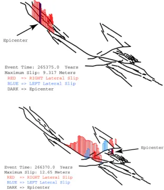
Event Time: 265375.0 Years Maximum Slip: 9.317 Meters
RED => RIGHT Lateral Slip
BLUE => LEFT Lateral Slip
DARK => Epicenter Epicenter
Figure 2a: Rundle et al 2006, HESS
Event Time: 266370.0 Years Maximum Slip: 12.65 Meters
RED => RIGHT Lateral Slip BLUE => LEFT Lateral Slip DARK => Epicenter
Epicenter
Figure 2b: Rundle et al 2006, HESS
Fig. 2. Illustration of simulated earthquakes on the San Andreas
fault. Two large earthquakes are shown. Panel (a) is an event that is reminiscent of the San Francisco earthquake of 1906 on the northern San Andreas fault. Panel (b) is an event that is similar to the Fort Tejon earthquake of 1857 on the southern San Andreas fault near the Big Bend between Fort Tejon and Wrightwood.
California and is illustrated in Fig. 1. In this version of the model, Virtual California is composed of 650 fault segments, each of which has a width of 10 km and a depth of 15 km. A much more detailed treatment and explanation of the dy-namics and equations solved numerically for Virtual Califor-nia simulations can be found in (Rundle et al., 2004, 2005, 2006a,b, and references therein).
An example of results from Virtual California is shown in Figs. 2a, b in which we show two large earthquakes, one rem-iniscent of the San Francisco earthquake of 1906 (Fig. 2a) on the northern San Andreas fault, and one similar to the Fort Tejon earthquake of 1857 on the southern San Andreas fault near the Big Bend between Fort Tejon and Wrightwood (Fig. 2b). In both Figs. 2a, b, red vertical bars represent “right lateral slip” (opposite side of the fault moves to the right) and blue vertical bars represent “left lateral slip”.
It can be seen in Fig. 2a that the earthquake on the North-ern San Andreas fault, where most of the slip occurs, also involves triggered slip on the Hayward, Rogers Creek and Maacama faults (these are the faults to the east of – “behind” – the main trace of the San Andreas fault). The dark bar on the San Andreas fault represents the epicentral segment, the segment that was the first to slip in the event. The maximum amplitude of slip, as shown in the figure, is 9.3 m.
Figure 2b shows a large event in southern California sim-ilar in extent and magnitude to the 1857 Fort Tejon earth-quake. It can be seen that while most of the slip occurs on the main trace of the San Andreas fault, where the maximum amplitude of slip is 12.6 m, other triggered slip occurs on the Big Pine fault, the Garlock fault, the San Gabriel fault, and faults in the Mojave desert and Owens Valley to the east. In fact, it is extremely interesting that all of this activity be-gan with initial slip on a small fault in the Mojave desert, as shown by the location of the dark epicentral vertical slip bar.
4 Patterns in Virtual California
We used 10 000 years of simulation data from Virtual Cal-ifornia to compute the N = 650 spatial patterns of activ-ity for the simulation. These patterns reveal which are the most dominant and important modes of correlated activity, and which are less important. The eigenvectors (spectrum) indicate the fraction of the eigenvectors that are present, on average, in the activity during the simulation. More specifi-cally, pn=λ2n, is the fraction of eigenvector qn(x) of the or-thonormal N × N matrix Q of Eq. (4) is present, on average, in the activity. Note that
N
P
n=1
pn=1. Using a frequency in-terpretation for probability, we can say that on average, over the 10 000 years of simulation data, the probability of finding eigenvector qn(x) in the data is on average pn.
In Figs. 3a, b, c, d we show the first four orthonormal cor-relation eigenvectors qn(x), again for the same 10 000 years of simulation data. In these figures, the red and blue bars cor-respond to locations where the value of qn(x) is significantly different from 0. The heights of the red and blue bars repre-sent the values of qn(x), and can take on values between −1. and +1. Red bars represent positive values of qn(x) between 10−3and 1, and blue bars represent negative values of qn(x) between −1 and −10−3. Green dashed lines are locations where |qn(x)| has a value less than 10−3, which is roughly the amplitude of the numerical error. The physical meaning of the red and blue colors for a particular eigenvector qn(x), which represents a particular fundamental pattern of activity is:
– Red sites tend to be active when other red sites are
ac-tive, so that activity at red sites is positively correlated with activity at other red sites;
– Blue sites tend to be active when other blue sites are
ac-tive, so that activity at blue sites is positively correlated with activity at other blue sites;
– Red sites tend to be inactive when the blue sites are
ac-tive and vice-versa, so that activity at red sites is nega-tively correlated with activity at other blue sites. Figure 3a is an eigenvector that represents the most important pattern of activity in the 10 000 years of simulation data. This
Figure 3a: Rundle et al 2006, HESS
Figure 3b: Rundle et al 2006, HESS
Figure 3c: Rundle et al 2006, HESS
Figure 3d: Rundle et al 2006, HESS
Fig. 3. This figure shows the first (and most important) four
corre-lation eigenvectors for 10 000 years of simucorre-lation data. The color-coding of the vertical bars is that: 1) Red sites tend to be active when other red sites are active, so that activity at red sites is positively cor-related with activity at other red sites; 2) Blue sites tend to be active when other blue sites are active, so that activity at blue sites is posi-tively correlated with activity at other blue sites; 3) Red sites tend to be inactive when the blue sites are active and vice-versa, so that ac-tivity at red sites is negatively correlated with acac-tivity at other blue sites.
794 J. B. Rundle et al.: Pattern dynamics, pattern hierarchies, and forecasting
Figure 4: Rundle et al 2006, HESS
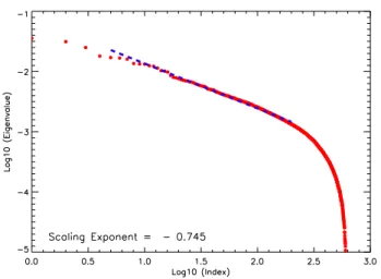
Fig. 4. Plot of the eigenvalue spectrum pn on a log-log plot.
Log10pnis plotted as a function of Log10n, where n is the index
number of the eigenvector (n=1 has the largest value of pn, and the
rest are ordered by descending values of pn).
pattern of activity comprises p1 =3.5%, on average, of the
activity over 10 000 years of simulations. It bears a strong resemblance to Fig. 2b, the 1857-type event. From Fig. 3a, it can be seen that this pattern is associated with correlated activity on the San Andreas, the Garlock and Big Pine, the Northern Mojave, the Owens Valley and Death Valley faults. If one were to expand the pattern of slip in Fig. 2b as a sum of the eigenvectors qn(x), the expansion coefficient q1(x) would
represent the most important term.
Figure 3b shows the second-most important eigenvector
q2(x). Here we primarily see strongly correlated activity
on the northern San Andreas, the Hayward-Rogers Creek-Maacama, the Calaveras and Bartlett Springs fault systems. This pattern of activity is seen in 3.1% of the activity over the 10 000 years of simulations. This eigenvector also resembles the event shown in Fig. 2a, the 1906-type event.
It is interesting that these first two patterns of activity are effectively decoupled between northern and southern Cali-fornia. The physical explanation for the decoupling is proba-bly related to the existence of the creeping zone of the central San Andreas fault. This zone is the ∼ 100 km long part of the San Andreas fault just to the north of the large slipped region in Fig. 2b. Earthquakes do not occur in the creeping zone, rather a steady aseismic slip is observed at a rate cor-responding to the long-term rate of plate motion across the fault, 35 mm/yr (Table 1). The creeping zone appears to act as a kind of “shock absorber” for the largest events, effec-tively eliminating the correlation of these events in the north and south.
Eigenvectors 3 and 4 are shown in Figs. 3c and d. Fig-ure 3c shows a pattern, representing 2.4% of the activity, characterized by correlated slip on the southernmost part of the faults of the San Andreas system, together with slip
ac-tivity on the eastern Garlock fault. Figure 3d is an interest-ing pattern, in which a kind of higher “pattern harmonic” of the activity on the faults of the northern San Andreas fault. Comparing Figs. 3b and d, eigenvector 4 (1.8% of the activ-ity) shows an anticorrelation between activity on the extreme northern end of the San Andreas system with the faults near the San Francisco Bay region (refer to Fig. 1 for locations relative to San Francisco). Eigenvector 4 also shows the be-ginnings of correlations between activity in northern Califor-nia with activity south of the creeping zone, on the eastern Garlock fault in the Mojave desert. Evidently the decoupling effect of activity in the north and south by the creeping zone of the San Andreas decreases as the higher pattern harmonics appear.
Figure 4 shows the eigenvalue spectrum pn. An index n enumerates all eigenmodes with decreasing importance as n increases. Here we plot log10(pn)as a function of log10(n).
We observe that there is a region of scaling or power-law behavior at values of n in the interval between n ∼ 10 and
n ∼200:
log10(pn) ∝ −.75 log10(n) (10 ≤ n ≤ 200) (5)
To understand this, we suppose that we can define a “char-acteristic wavelength” λn for each pattern according to the approximate ansatz:
λn∼ 2π L
n (6)
where L represents the linear size (length) of the largest events in the simulations. Then the scaling region shown in Fig. 4 must be an expression of the hierarchical nature of the spatial scale of the patterns generated by the fault system dy-namics:
pn∼λαn ∼n−α (7) The reason for the particular value of the scaling exponent
α = 0.745 ± 0.004 ≈ 0.75 is not at present known, but its value, which is nearly equal to the ratio of integers 3/4, would lead to the conjecture that it is related to the mean field nature of the dynamics (Rundle, 1989; Rundle and Klein, 1993; Tiampo et al., 2002a). In mean field dynamics, it is frequently the case that the scaling exponents are ratios of integers (see Klein et al., 2000).
We note that similar types of overall behavior for patterns has been observed in seismicity data (Tiampo et al., 2002b).
5 Conclusions
Forecasting in systems such as ENSO and earthquakes de-pends on the interpretation of observable space-time patterns, since the true stress-strain rate and stress-strain dynamics cannot be observed. It is likely that similar methods can be used for both systems, based upon the identification of pat-terns as eigenvectors of a dynamical correlation operator. We
note that these are linear descriptions of fundamentally non-linear dynamical systems. However, there are important ex-amples of probability distributions for nonlinear systems that are known to obey linear Fokker-Planck equations (Haken, 1983). Moreover, Klein et al. (2006)4show that the evolution of patterns in driven threshold systems can be characterized by correlation functions that have the properties discussed above.
We may speculate that hierarchical patterns that are ob-served in other nonlinear earth systems may be described in by similar methods. For example, it is known that in hydrol-ogy, river networks are observed to display scaling patterns that arise from purely local dynamics. These local dynam-ics include hill slope and topography, surface winds and ero-sion, and rainfall. Yet these local effects are often the product of long range interactions, i.e., correlation of hill slope and topography, and rainfall patterns over long distances (Tur-cotte, 1997). Moreover, the tree-like nature of river networks leads also to the conjecture that pattern hierarchies may have a mean field character, inasmuch as tree-like networks are of-ten found to be mean field constructs, such as the Bethe lat-tice in percolation theory (Stauffer and Aharony, 1994). Un-derstanding how these hierarchies of pattern scales develop and evolve doubtless holds the key to forecasting the future dynamical states of these systems.
Acknowledgements. This work has been supported by grant DE-FG02-04ER15568 from the U.S. Department of Energy, Office of Basic Energy Sciences to the University of California, Davis (J. B. Rundle, P. B. Rundle, G. Yakovlev); by grant DE-FG02-95ER14498 from the U.S. Department of Energy, Office of Basic Energy Sciences to the Boston University (W. Klein); grant ATM 0327558 from the National Science Foundation (D. L. Turcotte, R. Shcherbakov); and by grants from the Computational Technolo-gies Program of NASA’s Earth-Sun System Technology Office to the Jet Propulsion Laboratory, the University of California, Davis (J. B. Rundle, P. B. Rundle, A. Donnellan).
Edited by: M. Sivapalan
References
Broomhead, D. S. and King, G. P.: Extracting qualitative dynamics from experimental data, Physica D, 20, 217–236, 1986. Crouch, S. L. and Starfield, A. M.: Boundary Element Methods
in Solid Mechanics: with Applications in Rock Mechanics and Geological Engineering, George Allen & Unwin, London, 1983. Farrell, B.: Optimal excitation of neutral Rossby waves, J. Atmos.
Sci., 45, 163–172, 1988.
Haken, H.: Synergetics: An Introduction, Springer-Verlag, Berlin, 1983.
Holliday, J. R., Chen, C. C., Tiampo, K. F., Rundle, J. B., Turcotte, D. L., and Donnellan, A.: A RELM earthquake forecast based on pattern informatics, Seism. Res. Lett., in press, 2006.
Holmes, P., Lumley, J. L., and Berkooz, G.: Turbulence, Coherent Structures, Dynamical Systems and Symmetry, Cambridge Uni-versity Press, Cambridge, UK, 1996.
Jordan, T. F.: Linear Operators for Quantum Mechanics, John Wi-ley, New York, 1969.
Karner, S. L. and Marone, C.: Effects of loading rate and normal stress on stress drop and stick-slip recurrence interval, in: Geo-Complexity and the Physics of Earthquakes, edited by: Rundle, J. B., Turcotte, D. L., and Klein, W., Geophysical Monograph, 120, pp. 187–198, American Geophysical Union, Washington, D.C., 2000.
Klein, W., Anghel, M., Ferguson, C. D., Rundle, J. B., and Martins, J. S. S.: Statistical analysis of a model for earthquake faults with long-range stress transfer, in: GeoComplexity and the Physics of Earthquakes, edited by: Rundle, J. B., Turcotte, D. L., and Klein, W., Geophysical Monograph, 120, pp. 187–198, American Geo-physical Union, Washington, D.C., 2000.
Lay, T., Kanamori, H., Ammon, C. J., Nettles, M., Ward, S. N., Aster, R. C., Beck, S. L., Bilek, S. L., Brudzinski, M. R., But-ler, R., DeShon, H. R., Ekstrom, G., Satake, K., and Sipkin, S.: The great Sumatra-Andaman earthquake of 26 December, 2004, Science, 308, 1127–1133, 2005.
Penland, C.: Random forcing and forecasting using principal os-cillation pattern-analysis, Mon. Weather Rev., 117, 2165–2185, 1989.
Penland, C. and Sardeshmukh, P.: The optimal growth of tropi-cal sea surface temperature anomalies, J. Climate, 8, 1999–2024, 1995.
Penland, C. and Magorian, T.: Prediction of Nino 3 sea surface temperatures using linear inverse modeling, J. Climate, 6, 1067– 1075, 1993.
Penland, C. and Matrosova, L.: Studies of El Nino and inter-decadal variability in tropical sea surface temperatures using a non-normal filter, J. Climate, in press, 2006.
Preisendorfer, R. W.: Principal Component Analysis in Meteorol-ogy and Oceanography, edited by: Mobley, C. D., Develop. At-mos. Sci., 17, Elsevier, Amsterdam, 1988.
Rundle, J. B.: A physical model for earthquakes, 2, Application to southern California, J. Geophys. Res., 93, 6255–6274, 1988. Rundle, J. B.: A physical model for earthquakes: 3.
Thermodynam-ical approach and its relation to nonclassThermodynam-ical theories of nucle-ation, J. Geophys. Res., 94, 2839–2855, 1989.
Rundle, J. B. and Klein, W.: Scaling and critical phenomena in a class of slider block cellular automaton models for earthquakes, J. Stat. Phys., 72, 405–412, 1993.
Rundle, J. B., Klein, W., Tiampo, K. F., and Gross, S.: Linear pat-tern dynamics in nonlinear threshold systems, Phys. Rev. E., 61, 2418–2431, 2000.
Rundle, J. B., Tiampo, K. F., Klein, W., and Martins, J. S. S.: Self-organization in leaky threshold systems: The influence of near-mean field dynamics and its implications for earthquakes, neuro-biology, and forecasting, Proc. Nat. Acad. Sci., USA, 99, 2514– 2521., Suppl. 1, 2002a.
Rundle, J. B., Rundle, P. B., Klein, W., Martins, J. S. S., Tiampo, K. F., Donnellan, A., and Kellogg, L. H.: GEM Plate boundary simulations for the Plate Boundary Observatory: A program for understanding the physics of earthquakes on complex fault net-works via observations, theory and numerical simulation, Pure Appl. Geophys., 159, 2357–2381, 2002b.
Rundle, J. B., Rundle, P. B., Donnellan, A., and Fox, G.: Gutenberg-Richter statistics in topologically realistic system-level earth-quake stress-evolution simulations, Earth Planets Space, 56,
796 J. B. Rundle et al.: Pattern dynamics, pattern hierarchies, and forecasting 761–771, 2004.
Rundle, J. B., Rundle, P. B., Donnellan, A., Turcotte, D., Shcherbakov, R., Li, P., Malamud, B. D., Grant, L. B., Fox, G. C., McLeod, D., Yakovlev, G., Parker, J., Klein, W., and Tiampo, K. F.: A simulation-based approach to forecasting the next great San Francisco earthquake, Proc. Nat. Acad. Sci., 102, 15 363– 15 367, 2005.
Rundle, J. B., Rundle, P. B., Donnellan, A., Li, P., Klein, W., Mor-ein, G., Turcotte, D. L., and Grant, L.: Stress Transfer in Earth-quakes and Forecasting: Inferences from Numerical Simulations, Tectonophysics, 413, 109–125, doi:10.1016/j.tecto.2005.10031, 2006a.
Rundle, P. B., Rundle, J. B., Tiampo, K. F., Donnellan, A., and Tur-cotte, D. L.: Virtual California: Fault model, frictional param-eters, applications, Pure Appl. Geophys., doi:10.1007/s00024-006-0099-x, 2006b.
Rundle, P. B., Rundle, J. B., Tiampo, K. F., Martins, J. S. S., McGin-nis, S., and Klein, W.: Nonlinear network dynamics on earth-quake fault systems, Phys. Rev. Lett., 8714, Art. No. 148501, 2001.
Stauffer, D. and Aharony, A.: Introduction to Percolation Theory, Taylor and Francis, Bristol, PA, 1994.
Tiampo, K. F., Rundle, J. B., McGinnis, S., Gross, S., and Klein, W.: Mean field threshold systems and phase dynamics: An applica-tion to earthquake fault systems, Europhys. Lett., 60, 481–487, 2002a.
Tiampo, K. F., Rundle, J. B., Gross, S. J., McGinnis, S., and Klein, W.: Eigenpatterns in southern California seismicity, J. Geophys. Res., 107, B12, 2354, doi:10.1029/2001JB000562, 2002b. Tiampo, K. F., Rundle, J. B., Klein, W., Martins, J. S. S., and
Fer-guson, C. D.: Ergodic dynamics in a natural threshold system, Phys. Rev. Lett., 91, 238 501(1–4), 2003.
Travis, J.: Scientists’ fears come true as hurricane floods New Or-leans, Science, 309, 1656–1659, 2005.
Tullis, T. E.: Rock friction and its implications for earthquake pre-diction examined via models of Parkfield earthquakes, Proc. Nat. Acad. Sci. USA, 93, 3803–3810, 1996.
Turcotte, D. L.: Fractals and Chaos in Geology and Geophysics, 2nd Edition, Cambridge University Press, Cambridge, UK, 1997. Vautard, R. and Ghil, M.: Singular spectrum analysis in nonlinear dynamics, with applications to paleoclimate time series, Physica D, 35, 395–424, 1989.
Ward, S. N.: A synthetic seismicity model for southern California: Cycles, probabilities, hazards, J. Geophys. Res., 101, 22 393– 22 418, 1996.
Ward, S. N.: San Francisco Bay Area earthquake simulations: A step toward a standard physical earthquake model, Bull. Seis. Soc. Am., 90, 370–386, 2000.
Ward, S. N. and Goes, S. D. B.: How regularly do earthquakes re-cur – A synthetic seismicity model for the San Andreas fault, Geophys. Res. Lett., 20, 2131–2134, 1993.