Abstracts of the 2014 Brains, Minds, and Machines Summer School

(1)

CBMM Memo No. 024 September 26, 2014

Abstracts of the 2014 Brains, Minds, and Machines

Summer School

by

Nadav Amir, Tarek R. Besold, Rafaello Camoriano, Goker Erdogan, Thomas Flynn, Grant Gillary, Jesse Gomez, Ariel Herbert-Voss, Gladia Hotan, Jonathan Kadmon, Scott W. Linderman, Tina T.

Liu, Andrew Marantan, Joseph Olson, Garrick Orchard, Dipan K. Pal, Giulia Pasquale, Honi Sanders, Carina Silberer, Kevin A. Smith, Carlos Stein N. de Briton, Jordan W. Suchow, M.H.

Tessler, Guillaume Viejo, Drew Walker, and Leila Wehbe

Abstract: A compilation of abstracts from the student projects of the 2014 Brains, Minds, and Machines Summer School, held at Woods Hole Marine Biological Lab, May 29 - June 12, 2014.

This work was supported by the Center for Brains, Minds and Machines (CBMM), funded by NSF STC award CCF-1231216.

(2)

Abstracts of the

Brains, Minds, and Machines

2014 Summer School

Edited by

Andrei Barbu

Computer Science and Artificial Intelligence Laboratory, MIT

abarbu@mit.edu

Leyla Isik

Computational and Systems Biology, MIT

lisik@mit.edu

Emily Mackevicius

Brain and Cognitive Sciences, MIT

elm@mit.edu

Yasmine Meroz

School of Engineering and Applied Science, Harvard University

ymeroz@seas.harvard.edu

This work was supported by the Center for Brains, Minds and Machines (CBMM), funded by NSF STC award CCF-1231216.

(3)

Acknowledgments

We would like to thank all the instructors, speakers, and teaching fellows who participated in the Brains, Minds, and Machines course: Tomaso Poggio, L. Mahadevan, Gabriel Kreiman, Josh Tenenbaum, Nancy Kanwisher, Boris Katz, Shimon Ullman, Rebecca Saxe, Laura Schultz, Matt Wilson, Robert Desimone, Jim DiCarlo, Ed Boyden, Ken Nakayama, Patrick Winston, Lorenzo Rosasco, Sam Gershman, Lindsey Powell, Jed Singer, Jean Jacques Soltine, Marge Livingstone, Stefano Fusi, Larry Jackel, Cheston Tan, Tomer Ullman, Max Siegle, Ethan Meyers, Hanlin Tang, Hector Penagos, Andrei Barbu, Danny Harari, Alex Kell, Sam Norman-Haignere, Ben Deen, Stefano Anzellotti, Fabio Anselmi, Georgios Evangelopoulos, Carlo Ciliberto, and Orit Peleg.

We would also like to thank Grace Cho, Kathleen Sullivan, and Neelum Wong, as well as the Woods Hole Marine Biological Laboratory for all their hard work in organizing the course.

(4)

1 Modeling social reasoning using probabilistic

pro-grams

M. H. Tessler Jordan W. Suchow Goker Erdogan Stanford University Harvard University University of Rochester

Social inferences are at the core of human intelligence. We continually reason about the thoughts and goals of others — in teaching and learning, in cooperation and competition, and in writing and conversing, to name just a few. People are quick to make rich social inferences from even the sparsest data [2]. In this work, we draw on recent developments in probabilistic programming to describe social reasoning about hidden variables (such as goals and beliefs) from observed actions.

We consider the problem of inferring agents’ goals from their actions in a multi-agent setup where agents may or may not have shared interests. For example, suppose we observe that Alice and Bob go to the same meeting spot. Why did they do that? Were they trying to coordinate with each other? Or was Alice trying to avoid Bob, but was mistaken about where Bob was going to go? Or did Alice know where Bob usually went, but failed to realize that he was trying to avoid her, too? Some of these combinations of preferences and beliefs correspond to classic economic games — including coordination, anti-coordination, and discoordination games [3,4] — but the possibility of false beliefs and recursive reasoning allow for considerably richer scenarios and inferences, where agents reason not only about others’ actions in a given game [5], but also about the structure of the game itself.

To represent the richly structured knowledge that people bring to bear on social inferences, we built models using the probabilistic programming language Church [1]. For background and details on this form of model representation, seehttp://probmods.org.

We use a simplified setting where an agent selects actions according to a prior distribution. A utility function can then be used to update this prior distribution over actions into a posterior distribution; from a posterior distri-bution, a decision rule (e.g. probability matching or soft-max) can be used to generate actions. This is the process of inferring the action from planning for some goal, or generally, maximizing utility. In Church we could represent this as the following:

(def ine ( alice ) ( query

(def ine a l i c e - a c t i o n ( a c t i o n - p r i o r ) ) a l i c e - a c t i o n

( m a x - u t i l i t y ? a l i c e - a c t i o n ) ) )

where query is a special function in Church that performs conditioning. The first arguments to a query function are a generative model: definitions or background knowledge that we endow to the reasoning agent. Here, the generative model is very simple: aliceis trying to decide what action to take and she samples an action from a prior distribution over actions,(action-prior), which could be e.g. a uniform distribution over going out for Italian, Chinese, or Mexican food. The second argument, called the query expression, is the aspect of the computation about which we are interested; it is what we want to know. In this case, we want to know what Alice will do: what alice-actionwill be. The final argument, the conditioning expression, is the information with which we update our beliefs; it is what we know. Here, Alice is choosingalice-actionsuch thatmax-utility?is satisfied. We can define max-utilitylater to reflect Alice’s actual utility structure, whatever it may be.

In social situations, Alice’s utility may depend not only on her action, but what she thinks another person— let’s call him Bob—is likely to do. This could be formalized in the following way:(max-utility? alice-action (bob)). Because Bob is himself a reasoning agent, Alice’s model of Bob can be represented as a query function, just like our model of Alice.

(6)

(def ine ( bob depth ) ( query (def ine b o b - a c t i o n ( b o b - p r i o r ) ) b o b - a c t i o n (if (= depth 0) ( s e l f i s h - u t i l i t y ? b o b - a c t i o n ) ( m a x - u t i l i t y ? b o b - a c t i o n ( alice depth ) ) ) ) )

In this setup, Bob takes in an argument calleddepth, which specifies Alice’s depth of reasoning. If(= depth 0), Alice believes Bob will act according to the selfish part of his utility alone — he does what he wants without taking into account other people. If(= depth 1), Alice believes Bob is reasoning about what Alice will do, and her reasoning is of course dependent on what she thinks the selfish Bob will do. In this way, the probabilistic program is able to capture the recursive reasoning necessary for social cognitive tasks, e.g. coordination games.

We are interested not only in what actors will do but also what people will infer about the actors given their actions. We define anobserverfunction which reasons about Bob and Alice, and their intentions (here as utilities). (def ine o b s e r v e r

( query

(def ine a l i c e - u t i l i t i e s ( u t i l i t i e s - p r i o r ) ) (def ine b o b - u t i l i t i e s ( u t i l i t i e s - p r i o r ) ) (def ine ( alice depth ) ...)

(def ine ( bob depth ) ...) b o b - u t i l i t i e s

(and (= ( alice ...) o b s e r v e d - a l i c e ) (= ( bob ...) o b s e r v e d - b o b )

(= a l i c e - u t i l i t i e s r e v e a l e d - a l i c e - u t i l i t i e s ) ) ) )

Here, we are trying to inferbob-utilitiesfrom some observed actions:observed-aliceandobserved-bob, as well as what Alice has revealed to the observer in terms of her utilities. In these functions, we could substitute in that Bob has just gone to Alice’s favorite restaurant and/or that Alice has told us that she really wants to eat Italian. In this way, we are able to model inferences about a recursive reasoning process after observing some data. This basic model could be a foundation from which we construct intuitive theories of in-groups and out-groups, by inferring the intentions (which possibly could derive from group membership) of actors based on actions that themselves derive from intuitive theories of how others will behave.

References

[1] Noah D Goodman, Vikash K Mansinghka, Daniel M Roy, Keith Bonawitz, and Joshua B Tenenbaum. Church : a language for generative models Uncertainty in Artificial Intelligence, 2008.

[2] Fritz Heider and Marianne Simmel. An experimental study of apparent behavior. American Journal of Psychology, 57(2):243–259, 1944.

[3] Thomas C Schelling. The strategy of conflict. Harvard university press, 1980. [4] Colin Camerer. Behavioral game theory. New Age International, 2010.

(7)

2 Massive insights in infancy: Discovering mass &

mo-mentum

Kevin A. Smith Drew Walker Tarek R. Besold Tomer Ullman University of California University of California University of Osnabrück MIT

San Diego San Diego

By the time we are adults, we understand that some objects are heavier or denser than others, and how this "mass" property affects collisions between objects. For instance, based on only observing two objects colliding with one another, people can infer which is the more massive object in a way consistent with Bayesian inference over accurate, Newtonian physics (Sanborn, Mansinghka, & Griffiths, 2013). However, this rich knowledge of mass appears to be unavailable to newborns and infants. From the age of 3 months until 5 to 6 months, infants are not sensitive to relative sizes or masses – they expect any collision between a moving and resting object to send the resting object into motion equally (Baillargeon, 1998). By 9 months infants have an understanding of weight (preferring to play with lighter toys), but it is not until 11 months that they can infer the weight of an object based on how it interacts with other objects (e.g., how much it depresses a pillow it is resting on; Houf, Paulus, & Baillargeon, 2012). How do infants learn about the existence of hidden properties like mass during this period?

Here, we investigate what sorts of physical knowledge adults and infants must have to make the sorts of judgments that we know they are capable of. Recent research has suggested that people use an intuitive physics engine (IPE) that allows us to simulate how the world might unfold under various conditions of uncertainty, and make judgments based on those simulations (Battaglia, Hamrick, & Tenenbaum, 2013; Gerstenberg, Goodman, Lagnado, & Tenenbaum, 2012; Smith, Dechter, Tenenbaum, & Vul, 2013; Smith & Vul, 2013). We can therefore ask what object properties must be represented in an IPE to describe human judgments of mass. The IPE used here was implemented in Church (Goodman, Mansinghka, Roy, Bonawitz, & Tenenbaum, 2008) to allow for inference over latent attributes. In its fullest form, we assumed that people could noisily observe the position, size, and velocity of all objects on screen, but would need to infer the density and coefficients of friction and restitution (elasticity) by observing how those objects interact (see Figure1a).

We first tested whether this model could explain adults’ judgments of mass similarly to the model of Sanborn et al (2013): based on observing the incoming and outgoing velocities of two objects colliding, which of the two objects was heavier? Because the stimuli that Sanborn et al used were top-down views of direct collisions between boxes with no friction (following Todd & Warren, 1982), they used basic momentum transfer equations to describe the inference process people were using. An IPE would simplify to these equations given frictionless collisions, but we wanted to generalize these findings to somewhat more realistic stimuli: two balls colliding on a table with friction, from a side-on view. We therefore allowed the IPE model to observe collisions in which one ball would approach from the left and hit a stationary ball. In all cases, both balls were the same size, but the incoming ball was always heavier by one of four ratios (from Todd & Warren, 1982) – 1.25, 1.5, 2, or 3 times heavier. Likewise, we varied the elasticity of the collision to be 0.1 (very inelastic), 0.5, or 0.9 (very elastic). We could ask our IPE model to infer the mass of each ball based on the collision, and could then make probabilistic judgments about which ball was heavier. Despite the differences in the types of stimuli and the addition of friction, inference using an IPE shows a very similar pattern of results both to people (from Todd & Warren, 1982) and to the Sanborn et al (2013) model (see Figure1b-d).

While this suggests that the IPE can explain adults’ judgments of physics, it cannot explain the failures in physical reasoning that infants demonstrate. We therefore next ask what would be the minimum amount of physical knowledge needed to explain how infants make physical judgments. We focus initially on the finding that infants at 5-6 months are surprised when a smaller object launches a reference object farther than a larger one (Baillargeon, 1998). To do this, we presented the IPE model with two scenes in which a ball – larger in one scene and smaller in the other (see Figure2a) – hits a reference ball and asked the engine in which scene it believed the reference ball would travel farther. However, we also stripped out all latent attributes (density, friction, and elasticity) from

(8)

Figure 1: (a) Diagram of the intuitive physics engine. People observe noisy information about the position, size, and velocity each object and must infer mass (density), friction, and the coefficient of restitution based on how objects interact. (b-d) Probability of judging one object as heavier than another (y-axis) based on how much more massive that object is in reality (x-axis) after observing them collide. People (a) are biased by how elastic the collision is, which can be explained by the Sanborn et al (2013) model (c) and the IPE model (d).

this infant IPE. Instead, the infant IPE assumed that collision force was simply proportional to the size of the incoming ball (this is equivalent to assuming that all objects have the same density). Even with these simplifying assumptions, the infant IPE correctly judged that the bigger ball should cause the reference ball to go further, and this judgment became more accurate as the ratio of sizes between the two balls was increased (Figure2b).

However, such a simplified model cannot perform the rich physical inferences that adults and even older infants are capable of. If adults are shown videos of two collisions – one of a reference ball launching a large ball and one of the same reference ball bouncing off of a small ball (Figure3a) – they will naturally assume that the smaller ball is made of a dense material and the larger ball is made of something lighter. Since adults are inferring a general latent property (mass), they can use these inferences to answer many further questions about the balls in new environments.

We therefore propose a simple, novel experiment to test this idea. After seeing these collision events, adults would be able to transfer their knowledge of the masses of the balls and judge which would be more likely to knock down a tower of blocks if it rolled into it (e.g., Figure3b). However, if infants use size (not mass) to judge the force imparted in collisions, then they should be unable to make the same judgment. After infants transition to understanding that there is a latent mass or density attribute that objects have, on the other hand, they should be able to infer the differences between the balls and make the same judgment that the smaller, dense ball will be more likely to knock the tower down (as the IPE model can; Figure 3c). The ability to pass this predicted but undocumented developmental stage should correlate with the ability to perform other tasks related to mass inference (e.g, Houf et al., 2012).

While this work presents one potential trajectory along which knowledge of mass within collisions might develop, there remain significant outstanding questions about infants’ core conception of mass. Do infants initially understand that objects have mass that determines how they transfer momentum during collisions, but must learn about which objects are more or less massive? Or do infants need to learn that objects have the latent property of mass in the first place? It is only through further studies of infants’ physical understanding – such as the mass transfer experiment we suggested – that we will begin to understand how knowledge of our physical world develops into the useful, calibrated form that all adults have.

(9)

Figure 2: (a) The two scenes shown to the infant IPE model. The model was asked to "imagine" how the dynamics would unfold and judge which scene would cause the reference (right) ball to travel further. (b) The proportion of time the infant IPE model would judge the ball to travel farther in the first scene was a function of the ratio of the radii of the two launching balls.

Figure 3: (a) Two collisions are observed: a reference ball striking a larger ball and sending it quickly to the right, and the same reference ball striking a smaller ball and bouncing off. (b) The IPE model is then asked to imagine those same balls striking a tower and determine the probability that tower would fall. (c) The IPE model infers that the smaller, dense ball is much more likely to knock the tower down, as it judges that ball to have a much higher mass than both the reference ball (1 on the y-axis) and the larger, light ball.

(10)

References

Baillargeon, R. (1998). Infants’ understanding of the physical world. In M. Sabourin, F. Craik and M. Robert (Eds.), Advances in psychological science (Vol. 2, pp. 503-529). London: Psychology Press.

Battaglia, P., Hamrick, J., and Tenenbaum, J. (2013). Simulation as an engine of physical scene understanding. Proceedings of the National Academy of Sciences, 110(45), 18327-18332.

Gerstenberg, T., Goodman, N., Lagnado, D. A., and Tenenbaum, J. (2012). Noisy Newtons: Unifying process and dependency accounts of causal attribution. Paper presented at the Proceedings of the 34th Annual Meeting of the Cognitive Science Society, Sapporo, Japan.

Goodman, N., Mansinghka, V. K., Roy, D., Bonawitz, K., and Tenenbaum, J. B. (2008). Church: A language for generative models. Uncertainty in artificial intelligence.

Houf, P., Paulus, M., and Baillargeon, R. (2012). Infants use compression information to infer objects’ weights: Examining cognition, exploration, and prospective action in a preferential-reaching task. Child Development, 83(6), 1978-1995.

Sanborn, A. N., Mansinghka, V. K., and Griffiths, T. L. (2013). Reconciling intuitive physics and Newtonian mechanics for colliding objects. Psychological Review, 120(2), 411-437.

Smith, K. A., Dechter, E., Tenenbaum, J. B., and Vul, E. (2013). Physical predictions over time. Paper presented at the Proceedings of the 35th Annual Conference of the Cognitive Science Society, Berlin, Germany.

Smith, K. A., and Vul, E. (2013). Sources of uncertainty in intuitive physics. Topics in Cognitive Science, 5(1), 185-199.

Todd, J. T., and Warren, W. H. (1982). Visual perception of relative mass in dynamic events. Perception, 11, 325-335.

(11)

3 Aligning different imaging modalities when the

exper-imental paradigms do not necessarily match

Leila Wehbe Carnegie Mellon University

It is difficult to span a large portion of the stimulus space in a typical neuroimaging experiment because of the time constraints and the need to repeat stimuli to average out noise. Additionally, imaging modalities have different tradeoffs and none of them is strictly superior to the others. Magnetoencephalography (MEG) is a non-invasive tool that records the change in the magnetic field on the surface of the head and therefore has a very coarse spatial resolution. Intracranial Field Potentials (IFP) sample directly from the location of interest, but are invasive and only possible for use in humans when subjects are already undergoing surgery. As a result, there is a need to combine data from multiple experiments to increase the stimulus variety and benefit from the strengths of different modalities.

When different experiments do not share the same stimuli, the same modalities and the same subjects, how is it possible to combine them? Starting with an IFP and an MEG visual perception experiments that have similar but not the same stimuli, we show that we can align the two datasets by using the only dimension they have in common: time. This is a very first step towards integrating the two modalities and we compare between the alignment based on the time course and the one based on the stimuli properties.

Figure 4:[Left] Stimulus set for the IFP experiment in [3]. [Right] Stimulus set for the MEG experiment in [1].

Representational Similarity Analysis (RSA) [2] is a recent method to compare and find similarities in the rep-resentations of the same stimuli from different realms (for example, reprep-resentations of stimuli in a computational vision model versus in the human visual system). It relies on forming similarity matrices in both realms and com-puting their similarities. These square matrices have the same dimensions and each entry (i, j) corresponds to the similarity between stimuli i and j. It is therefore not possible to use this method with our datasets. Instead we compute a temporal similarity matrix: we bin the signal from both modalities into 10ms windows starting 100ms before stimulus presentation and ending 550ms after. For each sensor, we compute a similarity matrix in which each entry (i, j) corresponds to the similarity between time windows i and j, computed over all stimuli. Figure5

shows an example of these matrices for an IFP sensor and an MEG sensor. We then compute the similarities of the similarity matrices for each pair of IFP sensor and MEG sensor, effectively performing a Temporal Similarity Analysis (TSA).

Figure6 [Left] shows the results of the TSA between the MEG sensors and a middle occipital IFP sensor and an occipital pole IFP sensor. We notice that the same clusters of MEG sensors in the left visual regions are temporally related to the two relatively distant IFP electrodes, reflecting the fact that the MEG sensors sample from a large set of location.

The two datasets are not entirely different: we find in both pictures of faces, vegetables and vehicles. We can therefore do an approximate RSA by considering the three stimulus classes are the same in both experiments.

(12)

Figure6[Right] shows the results of this approximate RSA. We notice that now the two IFP sensors map to many regions in the brain. These different regions lie on different stages of the visual processing pathway and have a distinct representation for the three stimulus which is similar to the representation in the IFP sensors, perhaps because of the small sample size (3 stimulus classes). We conclude that TSA might be a more suitable approach to combine multimodal data.

Figure 5:Temporal similarity matrices for an IFP sensor (left) and an MEG sensor (right).

Figure 6: [Left] TSA between IFP and MEG data. Each box represents a different MEG sensor location compared to an IFP sensor (middle occipital or occipital pole (blue-red correspond to a scale from low-high, the lower part of the graph corresponds to the back of the head, left corresponds to left). [Right] Approximative RSA between the same middle temporal IFP sensor and occipital pole IFP sensor and different MEG sensor locations.

Acknowledgments

We thank Pablo Polosecki, Leyla Isik, Gabriel Kreiman, and Hanlin Tang.

References

[1] Leyla Isik, Ethan M Meyers, Joel Z Leibo, and Tomaso Poggio. The dynamics of invariant object recognition in the human visual system. Journal of neurophysiology, 111(1):91–102, 2014.

[2] Nikolaus Kriegeskorte, Marieke Mur, and Peter Bandettini. Representational similarity analysis–connecting the branches of systems neuroscience. Frontiers in systems neuroscience, 2, 2008.

[3] Hesheng Liu, Yigal Agam, Joseph R Madsen, and Gabriel Kreiman. Timing, timing, timing: fast decoding of object information from intracranial field potentials in human visual cortex. Neuron, 62(2):281–290, 2009.

(13)

4 Population dynamics in aIT underlying repetition

sup-pression

Jesse Gomez Stanford University

While the differences between circuits of computer and cortex are shrinking, primate visual cortex is still hallmarked by its plastic properties, able to update and alter its neural encoding scheme based on experience both recent and past. This is especially manifest in visual cortex, where repetitive presentation of a stimulus results in decreased neuronal firing and blood-oxygenation as measured with fMRI. This phenomenon, repetition suppression (RS), results in either unchanged or enhanced visual activity. The neural mechanisms underlying this counterintuitive relationship – diminished cortical activity and improved behavior – remain unclear. Using single-unit recordings from macaque anterior inferotemporal cortex (aIT), this project seeks to elucidate the dynamics of cortical activity induced by RS and link these plastic properties to invariant information processing within cortex.

Figure 7

A macaque was trained to passively fixate for 500ms before one of seven possible objects (guitar, car, couch, kiwi, flower, hand, face) was presented randomly in one of three peripheral locations (see Zhang et al., 2011). Each stimulus was presented 60 times for each of 132 sampled neurons. To examine the response time course as a function of stimulus repetition, we compare the smoothed summed population response for each. As illustrated in the top of Figure7 (responses to a guitar image shown for simplicity), there is a clear effect of RS whereby successive presentations result in a gradually decreasing peak of neural activity (darkest shade = first 10

(14)

presen-tations). Despite this attenuation in signal, a Poisson Naive Bayes classifier (Meyers, 2013) shows equivalent, if not enhanced, ability to categorize guitar trials in the first versus last 20 presentations (Figure 7, middle). One potential explanation for a global decrease in mean signal yet unimpaired classification is a reduction in variability, or increase in synchrony of neurons selective for a given stimulus. To test this, neural spike rates were calculated using the number of spikes of each guitar-selective neuron within a 300ms time window after stimulus onset. The correlations of the spike rates between different trials at the beginning of the experiment (first 20 trials) versus the end of the experiment (last 20 trials) were compared. The covariance of population-level activity across stimulus presentations was significantly higher in the late (r=.82) versus early (r=.74) presentations. An implication of de-creased variability is a drop in entropy. Calculating mutual information normalized by the number of spikes across the population across time (Figure 7, bottom) reveals that RS serves to enhance the amount of information per spike, allowing the population to enter a less metabolically demanding state while maintaining robust information about stimulus category. These findings were not observed for face stimuli (a category of stimulus for which this population of neurons was not selective). Thus, a drop in classification performance of non-preferred stimuli across repetition, and the concomitant decrease in uncertainty per spike for preferred stimuli, may offer evidence for a fatigue-sharpening model of RS whereby a global decrease in spike frequency with increased synchrony amongst neurons selective for the repeated stimulus may account for the phenomenon of RS.

(15)

5 Analysis of feature representation through similarity

matrices

Carlos Stein N. de Brito

Ecole Polytechnique Federale de Lausanne

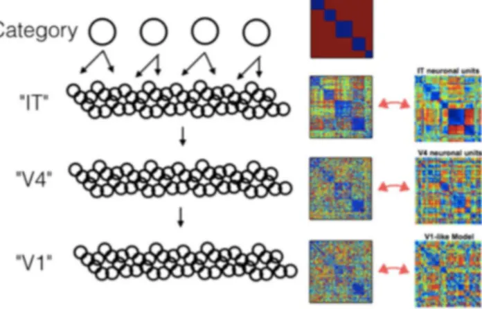
Multilayer, or deep, neural networks have succeeded in difficult object recognition tasks by mapping their input into high dimensional spaces, through a series of nonlinearities. The representation of the modeled neurons becomes more selective and invariant at each layer, from pixel representation, to textures and shapes, to object categories. Interestingly, through similarity matrices (SM), one can compare the representation of each layer to different cortical areas, e.g. V1, V4 and IT, upholding the idea that deep networks may be performing similar computations to the brain.

SMs estimate the distance between the representations of different input images for a model or population of neurons, and the comparison of SMs of different networks is used as a measure of representation similarity. Although an interesting measure, it is not clear what SM similarity tells us about neural representations. One cannot discard that indirect features, such as familiarity, object size or symmetry, could be the cause of different activations. Would networks with same architecture, but random connectivity, give the same results? Can neurons representing very different feature spaces have similar SMs? To be able to claim similar SMs as an indication of similar representations, one must have better understanding of its limitations.

We calculated the SM for different systems, including an ECoG dataset, a generative toy model and a high performance deep network. The ECoG data (Liu et al., 2009) for multi-trial exposure to five different visual stimuli shows that a block diagonal structure in the SM, indicating similar brain activity to the same stimulus category, peaks at 350ms after stimulus onset (Figure8). Although it indicates that the stimuli could be discriminated better at this time delay, it is agnostic as to what feature representation this brain activity signals.

To explore which kind of features would imply different SM structures, we implemented a simple multi-layer generative model. The model is a deep belief network with binary units, with the upper layer sampled first, from a mixture model (exactly one unit active), representing the stimulus category. Each unit has random sparse inputs from the lower layer, representing features. The same structure is repeated for each subsequent lower layer, with four in total, each having a factorial conditional probability distribution given the upper layer. This structure implies that units on upper layer are mostly active for single stimulus categories, while units in lower layers activate for multiple categories. The SM for trials ordered by stimulus category shows that the block diagonal structure is clear in the two highest layers, and dissipates gradually at each lower layer (Figure9).

(16)

Figure 9: SMs for a toy generative model and comparison with single unit data for visual stimuli (right column adapted from Yamins et al., 2014).

Figure 10: SMs for different layers of a deep network, with randomization between layer 3 and 4 at the bottom row.

We compare the model SMs to the SM of monkey single unit recordings at different stages of the visual cortex (Yamins et al., 2014). Higher visual areas are qualitatively similar to the higher layers of the generative model: both have block diagonal structure. This demonstrates how a feature class that has elements that are mostly active for a single category, as in the second upper layer of the toy model or in the monkey IT area, will imply a block diagonal structure, no matter which features have been sampled (the model’s features are abstract and random). Lower layers, in which features may be active for multiple categories, lose this property gradually.

Additionally, we ran a state-of-art 8-layer deep network (Krizhevsky et al., 2012, code from libccv.org), trained for object recognition, for five different object categories from ImageNet, and calculated the SM at each layer. As expected, a block structure gradually develops at higher layers. To test the importance of the specific representation, which is implemented in the connectivity, we randomized the connections between the third and forth layers (Figure

10). The new SMs have a similar structure at the forth layer, but fail to reproduce the block structure development later, in accordance with the probable loss of object recognition performance. Thus, having multi-layer network architecture is not enough to match neural SMs, and one must have the complex features that are discriminative.

These results indicate that the qualitative structure of the SM is an indication of the hierarchical level of representation, but does not specify which specific features are represented, as block diagonal structures appear for totally unrelated systems and stimuli sets. It does require that higher level features of the stimuli are represented, since random connectivity impedes the block diagonal structure. We may separate the two uses of SM comparison, as a qualitative visual similarity tool or quantitative distance measure. As a visual tool it serves as an indication of level of clustering across hierarchies, and should be compared to low-dimensional projections as a visualization of category clustering. Its power as a quantitative measure has not been investigated here, and it is still unclear what separates it from other linear projection measures, for example based on singular value decomposition. Further exploration should resolve these issues to precisely understand the power and limitations of SMs for representation comparison.

(17)

6 On Handling Occlusions Using HMAX

Thomas Flynn Joseph Olson Garrick Orchard

City University of New York Harvard University National University of Singapore

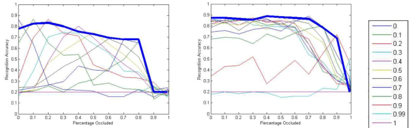
Recent years have seen great advances in visual object recognition with the availability of large training datasets and increased computational power making deep learning methods feasible. However, many object recognition models are still not robust to occlusions. Nevertheless, humans can robustly recognize objects under partial occlu-sion and we therefore know that the task is possible. This project was an initial approach to investigate the use of a bio-inspired model (HMAX) to handle occlusions. Five categories from the popular Caltech 101 database were chosen to investigate the performance of HMAX under occlusion. These categories were: Airplanes, Background, Cars, Faces, and Motorcycles. A common argument about recognition using the Caltech 101 database is that al-gorithms are not necessarily recognizing the objects themselves, but might be recognizing the scenes instead. For example, the algorithm may recognize roads rather than cars, and will use this to discriminate the Car class from others. To investigate whether HMAX was relying more on the background or objects themselves, we performed tests using two different types of occlusions. One which occludes the center of the image, and another which occludes the periphery. Figure11shows the different occlusions.

The standard HMAX model (Serre et al, 2007) was used to extract features which were then classified using a multiclass SVM classifier. 50 images were used per class, with 25 for training and 25 for testing. The results of classification are shown in Figure12. For central occlusions (Figure 12left) the classifiers always work best on images which have the same percentage occlusion as the examples they were trained on. However, the same is not true for peripheral occlusions (Figure12right), where most classifiers perform similarly well regardless of the percentage occlusion they were trained on.

The results suggest that the classifiers are relying more heavily on features extracted from the center of the image, which relates to the object (objects in the Caltech 101 database are always centered in the image). Accuracy of the classifiers degrades as the object in the image becomes more occluded. For central occlusions an increase in occlusion size causes a significant decrease in accuracy. However, for peripheral occlusions, increasing the occlusion size has little effect until the occlusion percentage surpasses 70%, at which stage the object in the center of the image is starting to be occluded.

For both types of occlusions, training the classifier using examples from all different percentages of occlusions provides the best overall results (thick blue lines in Figure12).

Occlusions themselves can introduce new features to the image. In the case of our occlusions, their edges elicit a strong response from the Gabor filters used in the first layer of HMAX. To reduce the effect of these introduced features, we post-processed the occluded images to "fill in" the occlusions. This was achieved by randomly selecting occluded pixels on the boundary and assigning to them the nearest non-occluded pixel value. This process was repeated until the entire occlusion was filled in. An example of a filled in occlusion is shown in

Figure 11: Illustration of the two different types of occlusion used. Far-Left: a Face image from the Caltech 101 database. Middle-Left: The same Face image occluded at the center. Middle-Right: the same Face image occluded at the periphery. Far-Right: a central occluded image with the occlusion later artificially filled in.

(18)

Figure 12: Accuracy of the HMAX model of a 5 class classification problem under varying percentages of oc-clusion. The left figure shows results for the center occlusion and the right figure shows results for periphery occlusion. The legend on the far right shows the percentage of occlusion on which the classifier was trained (re-sults for each classifier are shown as a separate plot). Thick blue lines indicate re(re-sults for a classifier trained on examples from from all different percentages of occlusion. Horizontal axis shows the percentage of the image occluded during testing.

Figure11.

To test on filled in occlusions, we trained the HMAX model with the procedure described above, and one image from each category was randomly chosen. All 5 of these images were initially classified correctly. Central occlusions were introduced to each image and the size of the occlusions were increased until the image was misclassified. For all 5 images the percentage occlusion at which classification failed roughly doubled when the occlusions were filled in.

Tang et al. (2014) measured field potential responses from neurons in the ventral visual stream to occluded images. They found that neurons responded 100ms later in the occluded condition compared to the whole condi-tion. This implies that the brain may need to perform recurrent processing in order to classify occluded objects. Motivated by this evidence, we tested if incorporating a recurrent Hopfield neural network as a top layer of the HMAX model would improve computational accuracy in classifying occluded objects (Hopfield, 1982).

We used Matlab’s built in Hopfield network program "Newhop". We seeded the network with 125 attractors – 25 for each class. The attracting points correspond to the C1 feature vectors extracted from HMAX. These vectors are 1024 dimensional. We then calculated nearest neighbor classification on 125 different test C1 feature vectors after allowing each vector to evolve in the network. We expected each test vector would converge onto one of the fixed attractors in the network. However, we observed the system to be unstable. The attractors themselves would not remain fixed, causing strange dynamics in the network. One consequence was that all of the test vectors would converge onto the same attractor resulting in 20% classification accuracy. We attribute this error to a flaw in our implementation of the Newhop program. We did confirm the program worked well when seeded with fewer (and lower dimensional) attractors. We repeated this analysis using features extracted from images with varying levels of occlusion as shown in Figure13.

We then computed nearest neighbor classification with the neighbor points being the points where our unstable attractors evolved to. This improved accuracy but, as seen in Figure13, this classification still performed no better than nearest neighbor classification directly on the C1 feature vectors without applying the Hopfield network. As Figure13also shows, increasing the amount of iterations within the Hopfield network before computing nearest neighbor actually decreases accuracy.

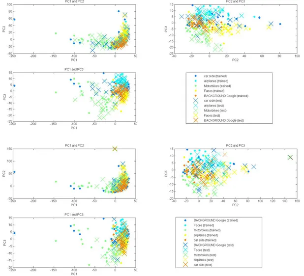
To make sure our C1 features made sense, we performed PCA on the features and found sufficient clustering of the vectors into classes – with the exception of the "background" class which was not clustered as expected due to the large variation in this class’ image content. We also performed PCA on occluded images and still observed clustering but the vectors moved towards the origin in PCA space. Presumably, as occlusion increases

(19)

Figure 13: Depicts the accuracy of the Hopfield network classifier as a function of the percent occluded images. Curves are shown for nearest neighbor classification (n.n.c.) directly on C1 feature vectors, n.n.c. after applying two steps of a Hopfield network, n.n.c. after two steps of an evolving Hopfield network where the set of nearest neighbors is now the points where the attractors moved to, and n.n.c. after ten steps of an evolving Hopfield network.

(20)

Figure 14: Top four: PCA analysis on the 125 (0% occluded) attractors represented by X’s and the 125 (0% oc-cluded) test vectors represented by dots. Bottom four: PCA analysis for 0% occluded attractors and 30% occcluded test vectors.

the vectors would move closer to the origin until they are fully occluded (they have no features) bringing them to the origin. The PCA plots are shown in Figure 14. We also calculated nearest neighbor classification using the PCA transformed vectors and accuracy was not improved (plots not shown). For future work, we recommend also incorporating other models of recurrent networks beyond the Hopfield network.

References

Serre T., Oliva A., Poggio T. A feedforward architecture accounts for rapid categorization (2007). Proceedings of the National Academy of Sciences 104 (15), 6424-6429

Tang, H, Buia, C, Madhavan, R, Crone, N, Madsen, J, Anderson, W.S., Kreiman, G. Spatiotemporal dynamics underlying object completion in human ventral visual cortex (2014). Neuron.

Hopfield, J.J. Neural networks and physical systems with emergent collective computational abilities (1982), Proceedings of the National Academy of Sciences of the USA, vol. 79 no. 8 pp. 2554–2558, April 1982.

(21)

7 What will happen next? Sequential representations in

the rat hippocampus

Nadav Amir Guillaume Viejo

The Hebrew University of Jerusalem Institut des Systèmes Intelligenets et de Robotique

The rat hippocampus has conventionally been known to provide information about the animal’s position in space via the firing rate of its place cells. However, more recent observations at finer time-scales suggest that the activity of these place cells provides information about sequences of locations as well. In this project we will explore the representation of sequential information in the rat hippocampus and more specifically ask whether the temporal pattern of activity in its cells contains information about the upcoming positions of the rat (i.e. "what will happen next?"). During the awake state, the rat hippocampus is known to exhibit two distinct "modes" of activity: sinusoidal EEG oscillations at 8-12Hz called theta rhythm and short-lasting (∼50-120ms) high-frequency (∼200Hz) oscillations called sharp wave ripples. The theta rhythm occurs when the rat is navigating or otherwise actively exploring its environment. Sharp wave ripples occur during periods of rest or immobility. In the first part of this project we study the sequential activity of hippocampal cells during theta oscillations and in the second part we explore the phenomena of "replay sequences": rapid, firing sequences occurring during the sharp wave ripples.

7.1 Phase Precession and Theta Sequences

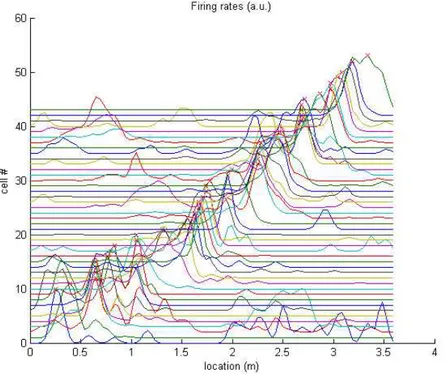
We first studied the phenomenon of hippocampal theta sequences using electrophysiological data (LFP and single unit spikes) recorded from the hippocampus of a rat navigating a linear track. It is well known that the activity of neurons in the hippocampus is spatially localized such that each neuron is active only when the rat occupies a certain area of the environment known as the cell’s place field (Figure15).

Figure 15: Firing rates of hippocampal place cells normalized and ordered by the maximal firing rate. More recently, it has been shown that the activity of these neurons ("place cells") exhibits a particular temporal relationship with the hippocampal theta rhythm (a 8-12Hz oscillatory EEG signal occurring at the hippocampus),

(22)

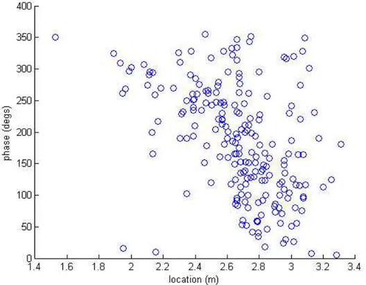
Figure 16: Relationship between spatial receptive field and theta rhythm for an example hippocampal neuron. Each point represents the phase of the theta oscillation and the rat’s position for an action potential fired by a place cell.

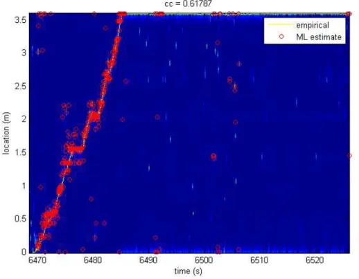
in which the spikes fired by each neuron occur at progressively earlier phases of the theta rhythm as the animal traverses the place field (Figure16). This relationship has been called phase precession and is believed to contribute to the occurrence of so called forward theta sequences: ordered sequences of place cell action potentials in which a portion of the animal’s spatial experience is played out in forwards order. Here we implemented a method for identifying the occurrence of standard (forward) as well as inverse (backwards) theta sequences based on the maximum likelihood estimate of the rat’s location. To estimate the rat’s location, we used the firing rate levels of the different place cells to and assuming they behave as independent Poisson neurons (Figure 17). Unlike the standard method of locating sequence events using correlation between time and cell order (in the place field sequence described earlier), here we defined forward sequences as four or more monotonically increasing place cell estimates occurring in the direction of the rat’s movement and backward sequences as four or more consecutive place cell estimates occurring in reverse order relative to the rat’s movement direction.

According to this new method of defining sequence events, it appears that forward sequences occur less of-ten than backward sequences (183 forward vs. 390 backward events). While the difference between number of forward and backward sequences is substantial, further analysis is required to compare the occurrence level of these sequences to chance levels. This could be done by counting the number of all other sequence permutations1 and checking whether forward and backward sequences occur significantly more (or less) frequently than other kinds of sequences. Furthermore, sequences should ideally be counted only when theta activity is actually present (i.e. when the power spectrum level of the Local Field Potential signal at the theta frequency range is above some threshold). In this preliminary study we used a velocity threshold criterion as a proxy for theta activity.

(23)

Figure 17: Empirical (solid lines) and maximum likelihood reconstruction (red circles) of the rat’s location. Note that location reconstruction is limited to periods in which the rat is moving.

7.2 Replay Sequences

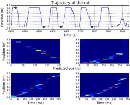
Previous studies have shown that when the rat is stationary at each end of the track, an activation of place cells occurs in a very short period of time. In the second part of this project, we applied the same (maximum-likelihood) decoding method used in the first part to the spiking activity that occurs during those periods of rest. As shown in Figure18, the decoding method predicts that the rat is running along the track in less than 400 milliseconds. Although the rat is stationary, these replay events have been characterized by several studies. For each replay event, we ordered the cells according to the position of their place fields along the track. The results are displayed in the top panel of Figure19. Clearly, the sequence of spikes follows the same order of the place fields when the rat is running along the track. The local field potential, filtered between 150 and 200 Hz, is also shown in Figure19. Consistent with previous studies, during replay events, we observed hippocampal ripples.

While the function of sequential activity in the hippocampus is still unknown, there appears to be ongoing place cell activity related to past events both during movement (in the form of backward theta sequences) and rest (in the form of replay sequences). While previous studies have emphasized the occurrence of forward sequences, hypothesizing they may relate to prediction of future events, the analysis carried out here indicates that back-ward sequences may be more common than forback-ward ones. However, further analysis is needed to determine the experimental conditions under which this observation holds, and the significance of each of these types of events.

(24)

Figure 18: Top panel: Position of the rat along the track as a function of time. Middle and bottom panel: Prediction of the position of the rat according to maximum likelihood reconstruction. The rat is stationary during times of rest, marked by green dots. Note that when the rat is at the right hand side of the track the sequence goes from right to left and vice versa.

Figure 19: Spiking activity (top panel) and local field potential (bottom panel) during a replay event. Note the correspondence between relative spike timings and the distribution of place fields from Figure15. Coincident with hippocampal replay, the LFP displays increased high frequency oscillations.

(25)

8 Discovering Latent States of the Hippocampus with

Bayesian Hidden Markov Models

Scott W. Linderman Harvard University

How do populations of neurons encode information about the external world? One hypothesis is that the firing rates of a population of neurons collectively encode states of information. As we interact with the world, gathering information and performing computations, these states are updated accordingly. A central question in neuroscience is how such states could be inferred from observations of spike trains, either by experimentalists studying neural recordings or by downstream populations receiving those spike trains as input.

This question has received significant attention in the hippocampus – a brain region known to encode infor-mation about spatial location [1]. Hippocampal “place cells” have the remarkable property that they spike when an animal is in a particular location in their environment. In this brief report, we analyze a 9 minute recording of 47 place cells taken from a rat exploring a circular open field environment roughly 1.2 meters in diameter. We first describe a sequence of Bayesian hidden Markov models (HMMs) of increasing sophistication and then show that: (i) these models capture latent structure in the data and achieve improved predictive performance over static models; (ii) nonparametric Bayesian models yield further improvements by dynamically inferring the number of states; (iii) even more improvement is obtained by modeling the durations between state transitions with a hidden semi-Markov model; and (iv) as expected, the latent states of the hippocampus correspond to spatial locations and can be used to decode the rat’s location in the environment.

Models

The fundamental building block of our spike train models is the hidden Markov model (HMM). It consists of a set of K latent states, an initial state distribution π, and a stochastic transition matrix A ∈ [0, 1]K×K. The proba-bility of transitioning from state k to state k0 is given by entry Ak,k0. The latent state in the t-th time bin is given

by zt∈ {1, . . . , K}. We observe a sequence of vectors xt ∈ ZN where xn,t specifies the number of spikes emitted by the n-th neuron during the t-th time bin. The spike counts are modeled as Poisson random variables whose means depend upon the latent state. We represent these rates with a vector λ(k)∈ RN _{where λ}(k)

n denotes the expected number of spikes emitted by neuron n when the population is in latent state k. Collectively, let Λ = {λ(k)}K

k=1. Together these specify a joint probability distribution,

p({xt, zt}tT=1| π, A, Λ) = p(z1| π) T

∏

t=2 p(zt| zt−1, A) T

∏

t=1 p(xt| zt, {λ(k)}Kk=1), p(z1| π) = Multinomial(z1| π), p(zt| zt−1, A) = Multinomial(zt| Azt−1,:), p(xt| zt, Λ) = N

∏

n=1 Poisson(xn,t| λ(znt)).

In order to specify our uncertainty over the parameters of this model, we use a Bayesian model with the following conjugate prior distributions,

π ∼ Dirichlet(α1), Ak,:∼ Dirichlet(α1), λ(k)n ∼ Gamma(a, b). We refer to this model as the Bayesian HMM.

(26)

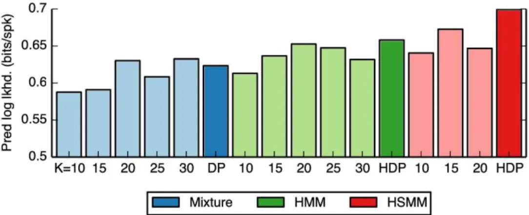
Figure 20: Predictive log likelihood of mixture models, hidden Markov models, and hidden semi-Markov models measured in bits per spike improvement over a baseline of independent time-homogeneous Poisson processes.

Typically, we also need to infer the number of latent states, K. One way to do so is to fit the Bayesian HMM for a variety of K and then choose the model with the best performance on a held-out validation dataset. An alternative approach is to use nonparametric Bayesian models such as the hierarchical Dirichlet process (HDP) as a prior distribution on the number of states. We omit the details of this model here and remark only that there exist a variety of approximate inference algorithms for fitting such models.

The final model variation that we consider is the hidden semi-Markov model (HSMM). In a standard HMM, the amount of time spent in state k is geometrically distributed as a function of Ak,k. In many real-world examples, however, the state durations may follow more interesting distributions. The negative binomial distribution provides a more flexible model for these state durations that can specify both the mean and the variance of how long we stay in a particular state. We can also derive a nonparametric extension called the HDP-HSMM with similarly efficient inference algorithms. An excellent description of these models and the algorithms for fitting them can be found in [2].

Results

With the HMM, we are expressing our underlying hypothesis that the hippocampus transitions between discrete states corresponding to different population firing rates. We test this hypothesis by training the model with 80% of the data (∼ 7 minutes) and testing on the remaining 20% (∼ 2 minutes). We measure performance with the predictive log likelihood, that is

log p(xtest| xtrain) = log

Z

π,A,Λ

p(xtest| π, A, Λ) p(π, A, Λ | xtrain) dπ dA dΛ.

For comparison, our baseline model is a set of independent, Poisson neurons with constant firing rate. The firing rate of each neuron is set to the total number of spikes observed during the training period divided by the time duration of the training period, in other words, the maximum likelihood estimate.

We also compare against a static “mixture of Poissons” model. In this model we have K mixture components characterized by firing rate vectors {λ(k)}K

k=1, and a component probability vector π ∈ [0, 1]

K _{that specifies how} likely each component is. This is essentially a hidden Markov model without couplings between the states at times t and t + 1, which is why we call this a “static” model. If this model were to perform as well as the HMM it would suggest that little information is encoded in the state transitions. As with the HMMs, we can incorporate a nonparametric, Dirichlet process prior on the number of components as well.

Figure20shows the results of our predictive log likelihood comparison. We find that the mixture models (blue bars) provide substantial gains over the baseline model, indicating that the firing rates are neither constant nor independent. Instead, there are a relatively small number of discrete “states” corresponding to different population

(27)

Figure 21: Top three states of the HDP-HSMM as measured by percentage of time spent in state. The left half of each plot shows the firing rate vectors, λ(k), with color intensities ranging from 0 to 16Hz. The right side shows the locations of the rat while in state k (black dots) along with their empirical probability density (shading) and the empirical mean (large colored circle). Clearly, the states are not uniformly distributed in space, but rather are localized to specific regions of the circular environment, as we would expect from a population of place cells.

firing rates. Incorporating Markovian transition dynamics between states with an HMM yields further improve-ments in predictive log likelihood (green bars), demonstrating that the state at time t can help predict the state in the next time step. Finally, modeling the duration of time spent in the same state with a hidden semi-Markov model yields even greater predictive performance (red bars). This likely corrects for a tendency of HMMs to quickly switch between states by allowing for some “stickiness” of the latent states. In this case we used a negative bi-nomial model for the state durations, which allows for durations that peak after some minimum time spent in the state.

Furthermore, we find that Bayesian nonparametric priors on the number of states (bold colored bars) outper-form their finite counterparts (lightly shaded bars) for the HMM and HSMM. Dirichlet process (DP) priors for the mixture models and hierarchical Dirichlet process (HDP) priors in the case of the HMM and HSMM automatically choose the number of states required to explain the data, and infer models that yield improved predictive perfor-mance. Interestingly, though the nonparametric models may effectively utilize the same number of states, they are inherently biased toward reusing latent states. This tendency can lead to better performance, even compared to finite models with the same number of utilized states.

How should we interpret the latent states of the HMMs? Since we are recording from hippocampal place fields, we expect these states to carry information about the rat’s location in his environment, and indeed that is what we find. Figure 21shows the empirical distribution over locations of the rat for each of the top three states of the HDP-HSMM, the model with the highest predictive performance. We see that when the rat is inferred to be in state k, it is typically located in a specific region of its circular environment. The black dots show the true location, and the colored shading indicates the empirical probability density obtained by binning those points in a circular distribution. The large, colored dots denote the mean of the empirical distributions. On the left of each plot we show the firing rate vector, λ(k)to illustrate the population firing rates in these states.

Given that these latent states correspond to the locations of the rat, we next investigate the “decoding” perfor-mance of the model, as in [3]. For each sample from the posterior distribution over HDP-HSMM parameters, we evaluate the marginal probability of each latent state for each test time bin. This tells us how likely each latent state is at each moment in time. Combining this with the empirical location distributions derived from the training data, illustrated in Figure21, we compute a distribution over the expected location of the rate during the test period. Finally, we average over samples from the posterior to derive the HDP-HSMM’s posterior mean estimate of the rat’s location during testing.

Figure22shows this posterior mean estimate in polar coordinates. Overall, the HDP-HSMM’s estimate (red line) does a fair job of tracking the rat’s true location (black line). It seems to estimate the angular position, θ(t), with higher accuracy than it does the distance from the center of the arena, r(t). Whether this discrepancy is due to the information content of the hippocampal spike trains remains an open question.

(28)

Figure 22: Decoded location of the rat during the held-out testing data, represented in polar coordinates.

We compare the decoding performance of the HDP-HSMM to an optimal linear decoder (blue line). In this model, the rat’s location (in Cartesian coordinates) is linearly regressed onto the spike trains. The resulting model fit accounts for correlations in the spike trains, and is the optimal linear decoder in that it minimizes mean squared error between the true and estimated training locations [4]. To be fair, when the linear model predicts a location outside the circular arena we project its estimate to the nearest point on the perimeter. Still, the posterior mean of the HDP-HSMM is a better decoder than the linear model, as can be seen by eye in Figure 22, and quantified in terms of mean squared error in the table below.

Model MSE

HDP-HSMM (posterior mean) 288cm2 Linear model 518cm2

Finally, in Figure 23 we investigate the HDP-HSMM’s predictive distributions over the rat’s instantaneous location. We look at three subsets of the testing data beginning at 15, 30, at 45 seconds into the testing period, respectively. For each subset, we plot the instantaneous location distribution taken at one second intervals. We show the instantaneous distribution over the location in colored shading, as well as the rat’s true location in five previous time bins (recall that the time bins are 250ms in duration) as black dots of increasing size and intensity. The largest dot indicates the true location at time t. We see that the instantaneous distributions are generally centered the rat’s true location, however, the spread of these instantaneous distributions suggests that the posterior mean estimator belies a fair amount of uncertainty. Whether this uncertainty arises from insufficient data, genuine uncertainty in location, or a misinterpretation of what these latent states truly encode, is a fascinating question for future study.

Conclusion

How the spiking activity of populations of neurons encodes information is largely an open question. This report has shown that there are statistically significant and predictable patterns in hippocampal spike trains that are well described by hidden Markov models. These models capture nonstationarities in neural firing rates and patterns in how firing rates transition from one time step to the next. Furthermore, by augmenting the HMM with two natural extensions — a nonparametric prior that effectively promotes the reuse of previous states, and a tendency to stick in the same state for extended periods of time — the models achieve even greater predictive performance. Finally, upon inspection of the inferred states of the HMM, we find that they correspond to locations in the rat’s circular environment, as we expected for this population of hippocampal place cells. With this observation, we can decode the rat’s location from spike trains alone.

A number of important scientific questions remain, however. Paramount among these is the question of model selection: how do we choose an appropriate model for spike trains? We have proceeded by hypothesizing models

(29)

Figure 23: Examples of the HDP-HSMM’s distribution of the instantaneous location of the rat during the testing period. Three sequences are shown; each sequence shows the instantaneous distribution evolving as the rat explores the environment. The black dots show the rat’s trajectory over the past second, with the largest, darkest dot showing the location at time t and the smallest dot showing the location at time t − 1. We see that the mean of the HDP-HSMM’s estimate is often close to the true location, but this may mask substantial uncertainty about the location.

of increasing sophistication to express our intuitions about how the hippocampus could encode different states of information. Our final model incorporates the likelihood of transitions between states, a bias toward reusing common states, and a tendency to persist in a particular state, but just because this model outperforms our other hypotheses does not mean it is optimal. For example, if we assume a priori that the population is representing location, then the model could leverage the constraints of a three dimensional world to inform the prior distribution over transition matrices.

Alternatively, if we begin with the assumption that this population is representing location, linear dynamical systems (also known as Kalman filters) are a natural alternative to HMMs. Essentially, linear dynamical systems are hidden Markov models with a continuous rather than a discrete latent state. As in this report, linear dynamical systems could be compared with HMMs in terms of predictive log likelihood and decoding accuracy to determine which better fits the data.

There are also technical questions related to how we should fit, or infer, the parameters of these models. Briefly, there are two main approaches, Markov chain Monte Carlo (MCMC), which we used here, and stochastic variational inference (SVI). Each has pros and cons in terms of computational cost and statistical accuracy that are

(30)

worth investigating in this application. From a neural perspective, these competing inference algorithms may also provide some insight into how a downstream population of neurons could interpret the hippocampal spike trains.

As we record from increasingly large populations of neurons, data driven tools for discovering latent structure in spike trains become increasingly vital. We have demonstrated how hidden Markov models and their extensions can discover significant, predictable, and interpretable latent structure in hippocampal spike trains. Armed with these tools, we can formulate and test hypotheses about neural encoding and computation in a general, flexible, and easily extensible manner.

Acknowledgments I would like to thank Zhe Chen and Matthew Wilson, with whom I have been collaborating on an extended version of this project, as well as Matt Johnson, who has given great advice and developed the excellent codebase that I built upon in this work. Finally, thank you to Tommy Poggio, L. Mahadevan, and the CBMM course TA’s for organizing an excellent summer school.

References

[1] John O’Keefe. A review of the hippocampal place cells Progress in neurobiology, 13(4):419–439, 1979.

[2] Matthew Johnson and Alan Willsky. Stochastic Variational Inference for Bayesian Time Series Models. Proceedings of The 31st International Conference on Machine Learning, 1854–1862, 2014.

[3] Emery N Brown, Loren M Frank, and Dengda Tang, and Michael C Quirk, and Matthew A Wilson. A statistical paradigm for neural spike train decoding applied to position prediction from ensemble firing patterns of rat hippocampal place cells. The Journal of Neuroscience,18(18):7411–7425, 1998.

[4] David K Warland, Pamela Reinagel, and Marcus Meister. Decoding visual information from a population of retinal ganglion cells. Journal of Neurophysiology,78(5):2336–2350, 1997.

(31)

9 Models of grounded language learning

Gladia Hotan Carina Silberer Honi Sanders Institute for Infocomm Research University of Edinburgh Brandeis University

Computational models of grounded language learning elucidate how humans learn language and can be used to develop image- and video-search systems that respond to natural language queries. We present a computational model which learns the meanings of verbs and nouns by mapping sentences to ‘perceived’ object tracks in natural videos, thus extracting meaningful linguistic representations from natural scenes. The computational task is to recognize whether a sentence describes the action shown in a particular video. Our approach assumes that all objects participating in the action of the video scene have already been recognized. We furthermore assume that the objects are represented as object tracks consisting of bounding boxes in each time frame. We focus on the recognition of transitive verbs and leave the recognition of prepositions, adjectives and adverbs for future work. In order to learn the meaning of verbs, we can train a HMM with three states. These states could be interpreted as the beginning, middle and end of an action. Likewise, we represent an object as another HMM with one state. Each state of the HMMs is associated with a probability distribution over observations, which we encode as features, such as the velocity of an object or the distance between two objects. We compute the feature values from the bounding boxes of the objects.

The video data consists of 97 videos, the bounding boxes of the detected tracks of four objects in total (back-pack, person, chair and ash-tray), and 259 sentence descriptions for the videos. For each verb, we train one HMM on all video-sentence pairs containing the corresponding verb, and it finds states and defines the emission prob-abilities (i.e. the relationship of that state with the features we observe) and the transition probprob-abilities between the states. This process results in states that are similar to those that a human would describe when defining that verb (Figure24). Thus the meanings of verbs are learned from labeled examples without predefining the relevant features.

Figure 24: The learned multidimensional gaussian distributions of observations for each state in the HMM for a verb are represented as a contour mesh at probability density=0.9. The observations corresponding to those states are similar to human descriptions of the verbs. For example, "approach" could be described as "first the objects are far from each other and not moving, then one object starts moving, and finally the objects are close to each other and not moving." The HMM also accurately identifies y-velocity as irrelevant for "approach" and x-velocity as irrelevant for "put down".

(32)

Figure 25: At each time point, the observations in the video can be compared with the emission probabilities of the states of the nodes in the factorial HMM to calculate the probability that the factorial HMM corresponding to the given sentence actually produced the observations from the given video.

Figure 26: Confusion matrix for the recognition of sentences containing a specific verb.

HMM, the identity of the nouns involved in the action are related to the observed features. The nouns can be trained independently and learn that the given object label is the most relevant parameter to object identity. Once the HMMs for individual verbs and nouns are trained independently, they can be put together given any sentence. The factorial HMM should then give a probability that the sentence describes the video.

In order to assess how well the factorial HMMs can learn to recognize sentences, we conducted an evaluation with 2-fold cross-validation. That is, we distributed the correct video-sentence pairs for each verb (36 each) to two sets and trained an HMM on one set. We tested the trained HMM on the other set plus all video-sentence pairs whose sentences are a false description of the video they are paired with. Afterwards we repeated the process with training and test sets swapped. Figure26shows the confusion matrix for the verbs approach and put down. The learnt HMMs are able to recognize almost all correct sentence descriptions for a given video and rejects almost all negative sentences which contain the respective other verb (second number in cell false-false). However, it fails to reject sentences with the correct verb but incorrect action participants.