HAL Id: ird-02063037
https://hal.ird.fr/ird-02063037
Submitted on 10 Mar 2019
HAL is a multi-disciplinary open access
archive for the deposit and dissemination of sci-entific research documents, whether they are pub-lished or not. The documents may come from teaching and research institutions in France or
L’archive ouverte pluridisciplinaire HAL, est destinée au dépôt et à la diffusion de documents scientifiques de niveau recherche, publiés ou non, émanant des établissements d’enseignement et de recherche français ou étrangers, des laboratoires
Can extinction rates be estimated without fossils?
Emmanuel Paradis
To cite this version:
Emmanuel Paradis. Can extinction rates be estimated without fossils?. Journal of Theoretical Biology, Elsevier, 2004, 229 (1), pp.19-30. �10.1016/j.jtbi.2004.02.018�. �ird-02063037�
Can extinction rates be estimated without fossils?
Emmanuel Paradis
∗Laboratoire de Pal´eontologie, Pal´eobiologie & Phylog´enie,
Institut des Sciences de l’ ´
Evolution,
Universit´e Montpellier II,
F-34095 Montpellier c´edex 05, France
Abstract
There is considerable interest in the possibility of using molecular phylogenies to estimate extinction rates. The present study aims at assessing the statistical performance of the birth–death model fitting approach to estimate speciation and extinction rates by comparison to the approach considering fossil data. A simulation-based approach was used. The diversification of a large number of lineages was simulated under a wide range of speciation and extinction rate values. The estimators obtained with fossils performed better than those without fossils. In the absence of fossils (e.g., with a molecular
phylogeny), the speciation rate was correctly estimated in a wide range of situations; the bias of the corresponding estimator was close to zero for the largest trees. However, this estimator was substantially biased when the simulated extinction rate was high. On the other hand the estimator of extinction rate was biased in a wide range of situations. Surprisingly, this bias was lesser with medium-sized trees. Some recommendations for interpreting results from a diversification analysis are given.
Keywords: Diversity; Estimation; Extinction; Maximum likelihood; Phylogeny;
1. Introduction
The tempo and mode of evolution has been one of the fundamental questions in evolutionary biology (Simpson, 1953). Recent advances in phylogenetics have given a fresh look at this issue (Barraclough and Nee, 2001). The reconstruction of the
relationships among species allows one to test whether the shape of the reconstructed phylogeny agrees with a given model of diversification (e.g., Kirkpatrick and Slatkin, 1993; Slowinski and Guyer, 1993; McKenzie and Steel, 2000). In the situation where the branches of the phylogeny have estimated lengths, it is possible to fit models in order to estimate the rates of diversification of the studied lineage (Nee et al., 1994b; Paradis, 1997).
Conceptually, the diversification of a lineage may be seen as a series of speciation and extinction events through time. Speciation events give birth to new species, and extinction events result in the death of species. This representation is practical for modelling the diversification of lineages since, with some further assumptions, this agrees with the birth-and-death processes which have been extensively studied in the past (Kendall, 1948a,b, 1949; Darwin, 1956; Keiding, 1975).
Nee et al. (1994b) proposed a method to estimate both speciation and extinction rates of a lineage using the reconstructed phylogenetic relationships of the living species, for instance using molecular data. They developed a likelihood-based approach to estimate both speciation and extinction rates. It follows that the extinction rate of a lineage could be estimated even in the absence of fossils, and thus without observing any event of extinction (Nee et al., 1995). This conjecture may seem counterintuitive since the information on extinction comes from extinct species: for instance, when a phylogeny with fossils is analysed, the estimation of extinction rate is done with the ratio of the number of extinction events on the cumulative numbers of species. Clearly, the number of extinction events cannot be observed without fossils.
Kubo and Iwasa (1995) developed a method close to Nee et al.’s (1994b): they used the same birth–death model but they fitted this model with a polytope algorithm instead of maximum likelihood. Kubo and Iwasa (1995) then showed, using simulations, that the estimator of extinction rates has a too large variance to be reliable.
It is important to assess the precision of the method introduced by Nee et al. (1994b) since it could have many potential applications in the study of organisms poorly
represented in the fossil record, such as soft-bodied organisms. This method may be used also to study the dynamics of viral populations (Nee et al., 1995). The goal of the present study is to assess the statistical performance of this method in a wide range of parameter values. Nee et al.’s (1994b) method performance was compared to the performance of the method where fossils, and thus past extinction events, are observed.
2. Methods
A large number of phylogenies were simulated with different values of speciation and extinction probabilities. The approach adopted was to simulate the speciation and extinction events, rather than generate sets of branching times from theoretical distributions, in order to mimic as close as possible the evolutionary process.
Simulations were started with a single species. At each time step, each species living in the lineage had a probability (denoted µ) to die. If it survived, each species had then a probability (denotedλ) to generate two daughter-species, otherwise it simply survived to the next time step. This process was simulated during 1000 time steps; all speciation and extinction events were recorded.
The probability of speciationλvaried between 0.0001 and 0.005 with a step of 0.0001, and for each of these values, µ varied between 0 andλ− 0.0001 with the same
step of 0.0001. The constraintλ> µ was imposed so that the risk of extinction of the
simulation was replicated 1000 times. Thus, a total of 2,500,000 simulations were started (50 values ofλ× 50 values of µ × 1000 replicates). Since the simulations were
fully stochastic, so were the number of species at any time step. The lineages with 0, 1, or 2 living species at the end of the simulation were discarded. For the other lineages, two phylogenies were recorded: the first one with all speciation and extinction events so that the extinct species are included, and the second one with only the species living at the end of the simulation.
The phylogenies with only the living species were analysed with Nee et al.’s (1994b) method. This method fits a birth–death process (Kendall, 1948b) to the set of branching times calculated from the phylogeny. A re-parametrization is needed to allow the model fitting so that the parameters under consideration are r =λ− µ, and a = µ/λ(see Nee et al., 1994b). The model is then fitted by maximum likelihood to give the estimates of both parameters, denoted ˆr and ˆa, respectively.
The phylogenies with the living and the extinct species were analysed with the method described by Keiding (1975) who gave the following two maximum likelihood estimators of the speciation and extinction rates:
ˆb = BT Z T 0 Xtdt , d =ˆ Z TDT 0 Xtdt , (1)
where BT is the number of speciation events between time 0 and T , DT is the number of
extinction events during the same time, and Xt is the number of species living at time t.
The integral at the denominators of eqn (1) was calculated as the sum of the branch lengths of the phylogeny.
The analyses of the simulated data were all done with R (Ihaka and Gentleman, 1996; R Development Core Team, 2003) using a package specially developed for phylogenetic analyses (Paradis et al., 2004). For all simulated lineages, the estimates ˆr, ˆa, ˆb, and ˆd
phylogeny without fossils (age of the youngest common ancestor of all living species). Note that the depth of the phylogeny with fossils was always 1000 time steps.
The relative error of each estimated parameter was calculated using: ˆr − (λ− µ) λ− µ , ˆ a − µ/λ µ/λ , ˆb −λ λ , ˆ d − µ µ . (2)
Using relative errors avoids having large errors due to the fact that the values of the parameter are large as well. In the simulations with µ = 0, the relative error of ˆa could
not be calculated and was replaced by its absolute error: ˆa − µ/λ. On the other hand, when µ = 0 the relative error of ˆd was not considered because there was no extinction
event (DT = 0), and thus ˆd = 0 in all replications.
Giving the very large amount of simulated data, summary statistics of the results were computed. The variations in the relative errors of the estimated parameters were investigated with respect to four variables: the true values ofλand µ, the number of tips of the phylogenies, and its depth. To give a picture of how the mean tendency and the dispersion of the relative errors varied, the results were summarized using
box-and-whiskers plots. The relative errors were first dispatched in different categories with respect to: (i) each value ofλ, (ii) each value of µ, (iii) an interval of the number of tips, or (iv) an interval of the depth of the tree. For the number of tips and the depth of the tree, the intervals were created with an algorithm in R in order to make categories with approximately similar numbers. The numbers of phylogenies analysed in each category are given in the Appendix.
In a second step, for each category a box-and-whiskers was drawn where the box represents the lower and upper quartiles (thus 50 % of the data are within the box), the median being indicated by a horizontal line inside the box. The upper and lower limits of the whiskers extend up to the quantiles Q0.05and Q0.95, respectively (so that 90 % of the
extreme outliers, particularly towards the positive values (data not shown), showing the extreme of these distributions with the whiskers (as usually done with such plots, Venables and Ripley 2002) would increase the range of the y-axis by several orders of magnitude, and would result in tiny unmeaningful boxes. These summary statistics were computed for each category ofλ, of µ, of the phylogeny depth, and of the number of tips of the phylogeny without fossils for the relative error of ˆr and the absolute error of ˆa.
They were also computed for each category ofλ, of µ, and of the number of tips of the phylogeny with fossils for the relative errors of ˆb and of ˆd.
To allow a more direct comparison of both kinds of estimators, estimates of the speciation and extinction rates without fossils (denoted ˆboand ˆdo, respectively) were
computed by back transformation of ˆr and ˆa:
ˆ do= ˆr ˆa 1 − ˆa, ˆ bo= ˆr + ˆdo. (3)
The relative errors of ˆboand ˆdowere calculated in the same way than for ˆb and ˆd.
To give a global picture of the bias in ˆboand ˆdo, the relative errors of these estimates
were plotted with respect to the number of tips of the analysed tree for different values of
λand of µ. Five values ofλwere selected (0.003, 0.0035, 0.004, 0.0045, and 0.005), and six values of µ (0, 0.0009, 0.0014, 0.0019, 0.0024, and 0.0029) for this analysis. A local polynomial fit (Venables and Ripley, 2002, p. 230) was performed on each plot.
3. Results
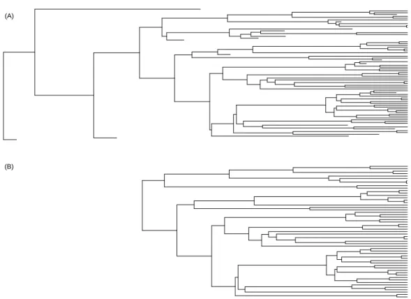
The 2,500,000 simulations yielded 604,165 lineages that were amenable to further analyses (that is they had at least three species living after 1000 times steps). Fig. 1 shows an example of such a simulated lineage with both derived phylogenies. Among the 604,165 phylogenies considering only living species, estimation of r and a was not possible in 112,083 cases (there was no convergence of the fitting algorithm). This
failure was clearly related to the number of tips in the tree: the mean number of tips among these 112,083 trees was 5.73 (sd = 2.94, median = 5, maximum = 32), whereas it was 31.63 (sd = 46.67, median = 16, maximum = 1140) among the 492,082 other trees.
The number of tips varied between 3 and 1140 for the phylogenies without fossils, and between 3 and 1161 for the phylogenies with fossils. In both cases, the distribution had its maximum at the smallest value, and was highly skewed towards the largest ones.
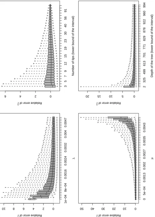
Fig. 2 shows the results for ˆr. There was a positive bias in this estimator for the smallest values ofλ, and the median of the relative error of ˆr converged to zero for increasing values ofλto be close to zero atλ≈ 0.002. The dispersion of the relative
error of ˆr also decreased with increasing values ofλ. The opposite results were observed with respect to the values of µ: the median of the relative error of ˆr was very large for the largest values of µ with a median of about 15 for µ = 0.0049. The median of the relative error of ˆr was somewhat unsensitive to the number of tips with just a small negative bias for the phylogenies with three tips. However, the dispersion of this error was greatly influenced by the number of tips: this dispersion decreased continuously for all
categories of number of tips. A positive bias in ˆr was observed when the depth of the tree was less than about 400 time units. This bias progressively decreased to zero when the depth of the tree increased. The dispersion of relative error of ˆr also decreased when the depth of the tree increased to stabilize at a depth of about 700 time units.
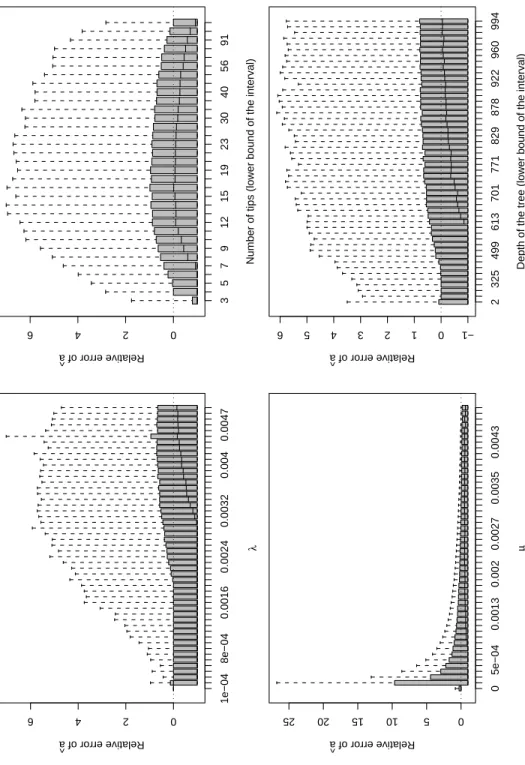
Fig. 3 shows the results for ˆa. With respect toλ, the relative error of ˆa was large for
the small values ofλand slowly converged to zero whenλincreased. The relative error
of ˆa was greatly affected by the value of µ: there was a systematic negative bias in ˆa
meaning that it underestimated the actual value of a in most situations. On the other hand, the dispersion of the relative error of ˆa decreased greatly with increasing values of
µ. The effect of the number of tips of the tree on ˆa was complex: there was a negative
numbers. The median of the relative error of ˆa was 0 for trees with 16 tips, but a negative
bias was observed for trees with more tips. With respect to tree depth, the median relative error of ˆa converged progressively to zero with increasing values of tree depth.
The dispersion of the relative error of ˆa was large for all values of tree depth.
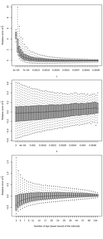
Fig. 4 shows the results for ˆb. The relative error of ˆb was very large for very small values ofλ, and its median quickly converged to zero with increasingλ. It is remarkable that the effect ofλon ˆb was very similar to that on ˆr with two differences, however: the dispersion of the relative error of ˆr was greater (forλ= 0.005, the first and third quartiles
were −0.118, 0.067 for ˆb, and −0.264, 0.160 for ˆr), and the median of the relative error of ˆb converged to zero more quickly though the difference was slight but systematic (for
λ= 0.0016, the median relative errors of ˆb and ˆr were 0.099 and 0.203, respectively).
The relative error in ˆb was only slightly affected by the value of the extinction rate with a small positive bias for the large values of µ. In all cases, the dispersion of ˆb was small with 50 % of the values being between −0.2 and 0.2. As previously for ˆr and ˆa, a
negative bias in ˆb for the smallest numbers of tips was observed. However, the dispersion of the relative error of ˆb was much smaller than for ˆr.
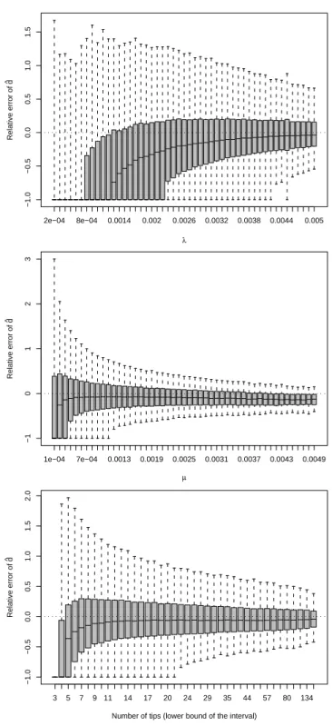
Fig. 5 shows the results for ˆd. The relative error of ˆd was greatly influenced byλ
with a strong negative bias for the smallest values of speciation rate and a progressive convergence of the median with increasing values. With respect to µ, there was a strong negative bias for the smallest values of extinction rate with a quick convergence to zero with increasing µ. However, a negative bias was observed for the largest values of µ. The dispersion of the relative error in ˆd continuously decreased with increasing values of µ.
As for the other estimators, the relative error in ˆd was affected by the number of tips in
the tree, but the dispersion was greater than for ˆb.
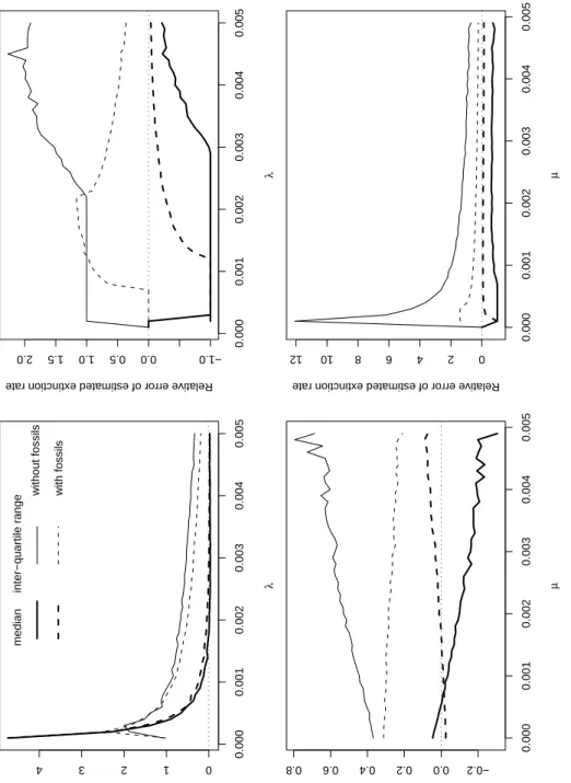
The estimates of speciation rate with (ˆb) and without ( ˆbo) fossils were compared for
estimators were very close except for the very small values ofλwhere the estimates with fossils were somehow better than without, though a positive bias was also observed for the former. In terms of dispersion (as measured by the inter-quartile range), the estimates with fossils were slightly better than without fossils, particularly for the largest values of
λ. With respect to µ, the performances were more contrasted. With fossils, the bias in ˆb was close to zero for all values of µ but showed a positive trend with increasing values of
µ. Without fossils, the bias in ˆboshowed a negative trend, and was much stronger than
for ˆb for the largest values of µ. The contrast was even stronger when considering the dispersion of the estimates: the dispersion of ˆbowas always stronger than the dispersion
of ˆb and increased with increasing values of µ, whereas the dispersion of ˆbodecreased
with increasing values of µ.
The same comparison was done between ˆd and ˆdo(Fig. 6). With respect toλ, there
was always a negative bias for both estimators, and they both converged to zero with increasing values ofλbut the convergence was much quicker for ˆd than for ˆdo. The
dispersion of these estimates showed opposite trends, though the results were somewhat more complicated. With fossils, the dispersion of ˆd increased with increasing values of
λ, but then decreased forλ> 0.0023. On the other hand, the dispersion of ˆdoincreased
for all values ofλ, though it reached a plateau for 0.0003 <λ< 0.0023. With respect to
µ, both estimators showed parallel results but the performances of ˆd were much better
than for ˆdo, in terms of bias (the median of the relative error of ˆd was much closer to zero
than the one of ˆdo) as well as in terms of dispersion of the estimates.
The analysis of the relative error of ˆbowith respect to the number of tips showed very
similar results for the different values ofλand µ (Fig. 7). In all cases the fitted curve was close to zero for a number of tips between 10 and 20 or more. The remarkable difference among the different plots was the maximum number of tips which was clearly related to the differenceλ− µ. All plots also showed similar results for the dispersion of the
relative error of the estimates with a range of values quite similar, and a decrease in dispersion with an increasing number of tips.
The same analysis for ˆdoshowed more complex results (Fig. 8). When µ = 0 the
dispersion of the relative error of ˆdo(as shown by the range of the y-axes) was very low,
and the fitted curves converged to zero with growing numbers of tips. On the other hand, when µ > 0 the fitted curves were almost always negative, increased with growing numbers of tips up to 10–20 tips, and then decreased afterwards. There was a continuous variation though from the smallest to the largest values of µ: positive values of the fitted curves were observed for µ = 0.0009, whereas the fitted curves were well below zero for
µ = 0.0029. The dispersion of the relative error of ˆdodecreased with increasing values of
bothλand µ.
4. Discussion
There is undoubtedly considerable interest in the possibility to use molecular
phylogenies (or any phylogeny inferred from extant species) to estimate extinction rates since this approach does not require to collect data through time. However, it is
necessary to assess the biases and limits of this approach which is the goal of this paper. The assessment of the bias of the estimators with fossils was done mainly for
comparison: since the lineages that went extinct before 1000 time steps were not considered, the biases of these estimators were not correctly estimated.
Overall, the estimators obtained with fossils (ˆb and ˆd) performed better than those
without fossils (ˆr and ˆa): the former had generally smaller bias and smaller variance than
the former. All four estimators performed better with increasing values of speciation rate which is obviously due to the fact that high values ofλresult in more speciation events in the simulated trees eihter with or without fossils. On the other hand, when the extinction rate was high, all estimators were biased since most trees went extinct and
thus only those with a low realized value of µ were effectively analysed.
All estimators behaved generally well with respect to the number of tips: the median errors were close to zero for 15 or more tips. However, the dispersion of all four
estimators was continuously influenced by the number of tips: it was lowest for the largest number of tips. An exception to this pattern was ˆa which showed a negative bias
for the lowest and highest numbers of tips. Clearly, more tips result in more data to analyse, and thus it is expected that the estimators are more accurate (median close to zero, and low dispersion). In the case of ˆa, the negative bias for the highest numbers of
tips may be due to the fact that most large trees were simulated with a low value of µ and a high value ofλ. Consequently, these trees had a very low ratioλ/µ (= a) which
critically affected the relative error of ˆa. It is noteworthy that this negative bias for the
highest numbers of tips was also observed when considering the absolute error of ˆa, but
was much slighter than for the relative error (results not shown).
In the trees without fossils, the most recent common ancestor to all living species (i.e. the root of the tree) varied randomly depending on the simulation. The median relative error of ˆr was close to zero for tree depth values of about 450 or more, whereas a value of about 900 or more was required to obtain a median error of ˆa close to zero. The
depth of a tree is clearly related to extinction rate: the highest the value of µ, the lowest the probability of a species appearing early in the simulation to survive until present.
It should be noted that all the results in this study were obtained with trees, either with or without fossils, which were known without error in terms of unlabelled topology and branch lengths. This is unlikely to be always true in real situations since there are many sources of error in estimating phylogenetic trees as clearly illustrated by various phylogenetic studies (see Whelan et al., 2001, for a review). If these errors in estimating trees are uniformly distributed along the tree, it should be expected that the median errors of the estimators studied here are not affected, though their dispersion are likely to
be increased since a supplementary source of variation is added. On the other hand, if a systematic bias in estimating the trees exists, this will add a bias in the estimators of diversification.
Another assumption of the present study was that all species of the lineage are included in the reconstructed phylogenies. This is likely to be untrue in real situations. With fossils, many species are likely to have not been fossilized and thus cannot be included in a possible phylogenetic study. Without fossils, it is rare to have all living species of a clade to be included in a phylogenetic reconstruction. In the context of testing for temporal variation in diversification, it was shown that missing taxa in phylogenies induce a bias resulting in a substantial increase in the type I error rate (Nee et al., 1994a; Pybus and Harvey, 2000). There has been no assessment of the possible bias of the estimators ˆr and ˆa when a phylogeny is incomplete. However, it could be
speculated from the present study that missing taxa may have an effect on the estimation of r and a. Removing randomly some species from a clade can be seen as similar to analysing a smaller clade with the same parametersλand µ. Thus the effects of missing species can be predicted from the effects of the number of tips observed on Figs. 7 and 8. Consequently, missing taxa in phylogenies are likely to bring about a negative bias in ˆr (and ˆbo), whereas the effect on ˆa (and ˆdo) would be more complex. In both cases, the
bias is likely to be slight if the number of missing species is low.
It appears that accurate estimation of both speciation and extinction rates can be achieved only with fossil data. In the absence of fossils (e.g., with a molecular phylogeny), only the difference between these rates (r) can be estimated with some accuracy in a wide range of situations, notably when the speciation rate is relatively large compared to the extinction rate. On the other hand, the estimation of a was inaccurate in a wide range of situation. This result was anticipated by Darwin (1956, p. 30) who stated that “If N1, . . . , Nk[the cumulative numbers of species] are the only observed quantities,
estimation of µ/λis likely to be very inaccurate since the range of values of µ/λgiving the same set N1, . . . , Nk with a reasonable probability is very large.” The present study
gives some empirical numerical support to Darwin’s logical argument. Remarkably, accurate estimation of a was achieved when the extinction rate was close to zero and the tree depth was close to the actual age of the lineage, suggesting that a may be correctly estimated only when the tree without fossils is close to the tree with fossils (i.e. the ‘real’ tree of the lineage).
An unexpected result comes from the fact that the error in ˆdoincreases with
increasing number of tips in the tree (Figs. 7–8). By contrats to ˆa, this cannot be
explained by the fact that larger trees are produced by larger values ofλ(see above). It seems rather that large trees produced with a moderate value of µ do not show a typical distribution of their branch lengths. This is further evidenced by the fact that trees with a moderate number of tips (≈ 20) gave good results in terms of relative error of ˆdo. Using
the formula for the expected mean number of species in a clade after a time T , e(λ−µ)T (Kendall, 1948b), it can be found that a clade with an expectation of 20 species after
T = 1000 is characterized byλ− µ ≈ 0.003.
5. Conclusions and Recommendations
The results from the present study can be used to define recommendations when
interpreting an analysis of diversification. It is generally not possible to choose between both situations considered here, with or without fossils. Lineages with fossil data are often extinct, and those which are studied with a molecular phylogenetic approach usually have no or a poor fossil record. Indeed, the comparison between both kinds of estimators was not intended to define guidelines but to give a comparison for the estimators without fossils.
introduce a negative bias in the estimation ofλ, and an undetermined bias for µ. A clade with at least 15 species is appropriate to estimateλ. This parameter is likely to be underestimated with smaller trees. Surprinsingly, µ is likely to be well estimated with medium-sized trees (with 10–20 species). However, µ is likely to be underestimated in most situations except if µ ≈ 0 where an overestimation is expected. In the latter case, the bias will be very small though. In all cases, it seems better to consider ˆdoas a lower
bound of µ.
If some informations are available on the age of the studied clade and the age of the most recent common ancestor of the species included in the phylogeny (called tree depth in the present paper), this may be used in interpreting the estimates of speciation and extinction rates. If the ratio of the latter on the former is less than 0.5, then the estimate ofλis likely to be positively biased. If this ratio is less than 0.9, then the estimate of µ is likely to be negatively biased.
The present study is the first extensive analysis of the statistical performance of the birth–death estimators as applied to phylogenetic data. Nee (2001) used simulations to compare the statistical properties of several estimators but he considered only the birth–only model (also called Yule model). Some further studies are clearly needed, particularly to assess the robustness of the birth–death estimators when rates vary through time or across lineages since such situations are likely to be more biologically plausible than the homogeneous rates case considered here.
Acknowledgements
I am grateful to two anonymous referees for their constructive comments on a previous of this paper. This research was financially supported by the Institut Franc¸ais de la Biodiversit´e and the Centre National de la Recherche Scientifique. This is publication 2004-009 of the Institut des Sciences de l’ ´Evolution (Unit´e Mixte de Recherche 5554 du
Centre National de la Recherche Scientifique).
Appendix
T able A1. Number of simulated lineages with respect to each value of speciation rateλ.
λ Number of trees λ Number of trees
0.0001 10 0.0026 12094 0.0002 52 0.0027 12717 0.0003 192 0.0028 13245 0.0004 339 0.0029 13883 0.0005 639 0.003 14553 0.0006 934 0.0031 15066 0.0007 1277 0.0032 15729 0.0008 1690 0.0033 16242 0.0009 2054 0.0034 17044 0.001 2648 0.0035 17528 0.0011 3061 0.0036 18165 0.0012 3602 0.0037 18581 0.0013 4261 0.0038 19304 0.0014 4755 0.0039 19701 0.0015 5346 0.004 20505 0.0016 5998 0.0041 21036 0.0017 6526 0.0042 21535 0.0018 7056 0.0043 21881 0.0019 7707 0.0044 22362 0.002 8331 0.0045 32434 0.0021 8886 0.0046 23821 0.0022 9691 0.0047 24213 0.0023 10194 0.0048 24312 0.0024 10849 0.0049 24990 0.0025 11513 0.005 25613
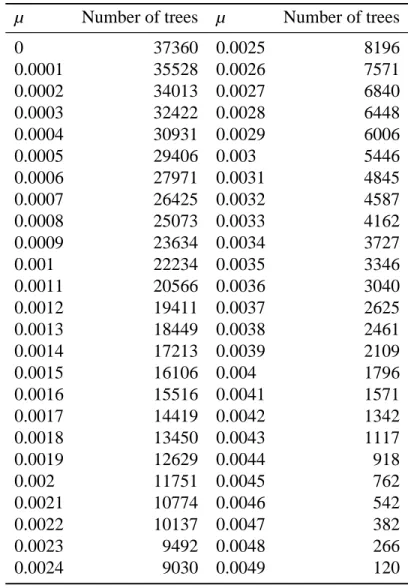
Table A2. Number of simulated lineages with respect to each value of extinction rate µ.
µ Number of trees µ Number of trees
0 37360 0.0025 8196 0.0001 35528 0.0026 7571 0.0002 34013 0.0027 6840 0.0003 32422 0.0028 6448 0.0004 30931 0.0029 6006 0.0005 29406 0.003 5446 0.0006 27971 0.0031 4845 0.0007 26425 0.0032 4587 0.0008 25073 0.0033 4162 0.0009 23634 0.0034 3727 0.001 22234 0.0035 3346 0.0011 20566 0.0036 3040 0.0012 19411 0.0037 2625 0.0013 18449 0.0038 2461 0.0014 17213 0.0039 2109 0.0015 16106 0.004 1796 0.0016 15516 0.0041 1571 0.0017 14419 0.0042 1342 0.0018 13450 0.0043 1117 0.0019 12629 0.0044 918 0.002 11751 0.0045 762 0.0021 10774 0.0046 542 0.0022 10137 0.0047 382 0.0023 9492 0.0048 266 0.0024 9030 0.0049 120
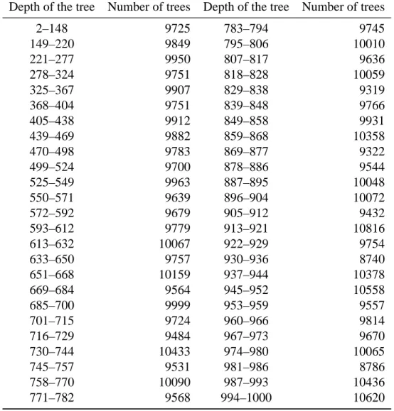
Table A3. Intervals defined to make groups with respect to the depth of the tree for the
phylogenies without fossils.
Depth of the tree Number of trees Depth of the tree Number of trees
2–148 9725 783–794 9745 149–220 9849 795–806 10010 221–277 9950 807–817 9636 278–324 9751 818–828 10059 325–367 9907 829–838 9319 368–404 9751 839–848 9766 405–438 9912 849–858 9931 439–469 9882 859–868 10358 470–498 9783 869–877 9322 499–524 9700 878–886 9544 525–549 9963 887–895 10048 550–571 9639 896–904 10072 572–592 9679 905–912 9432 593–612 9779 913–921 10816 613–632 10067 922–929 9754 633–650 9757 930–936 8740 651–668 10159 937–944 10378 669–684 9564 945–952 10558 685–700 9999 953–959 9557 701–715 9724 960–966 9814 716–729 9484 967–973 9670 730–744 10433 974–980 10065 745–757 9531 981–986 8786 758–770 10090 987–993 10436 771–782 9568 994–1000 10620
Table A4. Intervals defined to make groups with respect to the number of tips for the
phylogenies without fossils.
Number of tips Number of trees
3 59722 4 48139 5 40003 6 33835 7 29442 8 25660 9 22400 10 19911 11 17906 12 16161 13 14633 14 13302 15 12216 16 11239 17–18 20104 19 8789 20–21 16094 22 7146 23–24 13327 25–26 11832 27–29 15463 30–32 13040 33–35 11353 36–39 12918 40–43 11001 44–49 13620 50–55 11029 56–64 13048 65–75 12049 76–90 11885 91–114 12367 115–161 12315 162–1140 12216
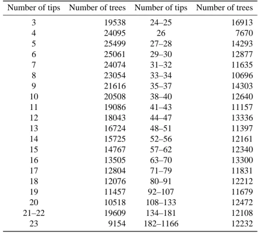
Table A5. Intervals defined to make groups with respect to the number of tips for the
phylogenies with fossils.
Number of tips Number of trees Number of tips Number of trees
3 19538 24–25 16913 4 24095 26 7670 5 25499 27–28 14293 6 25061 29–30 12877 7 24074 31–32 11635 8 23054 33–34 10696 9 21616 35–37 14303 10 20508 38–40 12640 11 19086 41–43 11157 12 18043 44–47 13336 13 16724 48–51 11397 14 15725 52–56 12161 15 14767 57–62 12340 16 13505 63–70 13300 17 12804 71–79 11831 18 12076 80–91 12212 19 11457 92–107 11679 20 10518 108–133 12472 21–22 19609 134–181 12108 23 9154 182–1166 12232 References
Barraclough, T. G., Nee, S., 2001. Phylogenetics and speciation. Trends Ecol. Evol. 16 (7), 391–399.
Darwin, J. H., 1956. The behaviour of an estimator for a simple birth and death process. Biometrika 43, 23–31.
Ihaka, R., Gentleman, R., 1996. R: a language for data analysis and graphics. J. Comput. Graph. Statist. 5 (3), 299–314.
Keiding, N., 1975. Maximum likelihood estimation in the birth-and-death process. Ann. Stat. 3 (2), 363–372.
Kendall, D. G., 1948a. On some modes of population growth leading to R. A. Fisher’s logarithmic series distribution. Biometrika 35 (1), 6–15.
Kendall, D. G., 1948b. On the generalized “birth-and-death” process. Ann. Math. Stat. 19, 1–15.
Kendall, D. G., 1949. Stochastic processes and population growth. J. R. Statist. Soc. B 11 (2), 230–264.
Kirkpatrick, M., Slatkin, M., 1993. Searching for evolutionary patterns in the shape of a phylogenetic tree. Evolution 47 (4), 1171–1181.
Kubo, T., Iwasa, Y., 1995. Inferring the rates of branching and extinction from molecular phylogenies. Evolution 49 (4), 694–704.
McKenzie, A., Steel, M., 2000. Distributions of cherries for two models of trees. Math. Biosci. 164, 81–92.
Nee, S., 2001. Inferring speciation rates from phylogenies. Evolution 55 (4), 661–668. Nee, S., Holmes, E. C., May, R. M., Harvey, P. H., 1994a. Extinction rates can be
estimated from molecular phylogenies. Phil. Trans. R. Soc. Lond. B 344, 77–82. Nee, S., Holmes, E. C., Rambaut, A., Harvey, P. H., 1995. Inferring population history
from molecular phylogenies. Phil. Trans. R. Soc. Lond. B 349 (1327), 25–31.
Nee, S., May, R. M., Harvey, P. H., 1994b. The reconstructed evolutionary process. Phil. Trans. R. Soc. Lond. B 344, 305–311.
Paradis, E., 1997. Assessing temporal variations in diversification rates from phylogenies: estimation and hypothesis testing. Proc. R. Soc. Lond. B 264, 1141–1147.
Paradis, E., Claude, J., Strimmer, K., 2004. APE: analyses of phylogenetics and evolution in R language. Bioinformatics 20 (2), 289–290.
Pybus, O. G., Harvey, P. H., 2000. Testing macro-evolutionary models using incomplete molecular phylogenies. Proc. R. Soc. Lond. B 267, 2267–2272.
R Development Core Team, 2003. R: a language and environment for statistical computing. R Foundation for Statistical Computing, Vienna, Austria, iSBN 3-900051-00-3.
URLhttp://www.R-project.org
Simpson, G. G., 1953. The major features of evolution. Columbia University Press, New York.
Slowinski, J. B., Guyer, C., 1993. Testing whether certain traits have caused amplified diversification: an improved method based on a model of random speciation and extinction. Am. Nat. 142 (6), 1019–1024.
Venables, W. N., Ripley, B. D., 2002. Modern applied statistics with S (fourth edition). Springer, New York.
Whelan, S., Li`o, P., Goldman, N., 2001. Molecular phylogenetics: state-of-the-art methods for looking into the past. Trends Genet. 17 (5), 262–272.
(A)
(B)
Figure 1: Illustration of the two phylogenies derived from the simulation of a lineage with speciation rateλ= 0.005 and extinction rate µ = 0.001. (A) Complete phylogeny
with the extinct species. (B) Phylogeny with only the species living at the end of the simulation. Note that the three most ancient species have disappeared from the data in (B). The parameter estimates for these data are: (A) ˆb = 0.0058, ˆd = 0.0015, and (B)
1e−04 8e−04 0.0016 0.0024 0.0032 0.004 0.0047 0 2 4 6 8 10 λ Relative error of r^ 0 5e−04 0.0013 0.002 0.0027 0.0035 0.0043 0 10 20 30 40 50 µ Relative error of r^ 3579 1 2 1 5 1 9 2 3 3 0 4 0 5 6 9 1 0 2 4 6
Number of tips (lower bound of the interval)
Relative error of r^ 2 325 499 613 701 771 829 878 922 960 994 0 5 10 15 20
Depth of the tree (lower bound of the interval)
Relative error of r^
Figure 2: Results for ˆr. On each plot, the effect is considered alone and the trees are combined for all the different values of the other effects (e.g., the trees with the same value ofλmay have different number of tips).
1e−04 8e−04 0.0016 0.0024 0.0032 0.004 0.0047 0 2 4 6 λ Relative error of a ^ 0 5e−04 0.0013 0.002 0.0027 0.0035 0.0043 0 5 10 15 20 25 µ Relative error of a ^ 3579 1 2 1 5 1 9 2 3 3 0 4 0 5 6 9 1 0 2 4 6
Number of tips (lower bound of the interval)
Relative error of a ^ 2 325 499 613 701 771 829 878 922 960 994 −1 0 1 2 3 4 5 6
Depth of the tree (lower bound of the interval)
Relative error of a ^
Figure 3: Results for ˆa. On each plot, the effect is considered alone and the trees are
combined for all the different values of the other effects (e.g., the trees with the same value ofλmay have different number of tips).
1e−04 7e−04 0.0013 0.0019 0.0025 0.0031 0.0037 0.0043 0.0049 02468 1 0 λ Relative error of b ^ 0 4e−04 0.001 0.0016 0.0022 0.0028 0.0034 0.004 0.0046 −0.6 −0.4 −0.2 0.0 0.2 0.4 0.6 µ Relative error of b ^ 3 5 7 9 11 14 17 20 24 29 35 44 57 80 134 −0.5 0.0 0.5 1.0 1.5
Number of tips (lower bound of the interval)
Relative error of b
^
Figure 4: Results for ˆb. On each plot, the effect is considered alone and the trees are combined for all the different values of the other effects (e.g., the trees with the same value ofλmay have different number of tips).
2e−04 8e−04 0.0014 0.002 0.0026 0.0032 0.0038 0.0044 0.005 −1.0 −0.5 0.0 0.5 1.0 1.5 λ Relative error of d ^ 1e−04 7e−04 0.0013 0.0019 0.0025 0.0031 0.0037 0.0043 0.0049 − 1 0123 µ Relative error of d ^ 3 5 7 9 11 14 17 20 24 29 35 44 57 80 134 −1.0 −0.5 0.0 0.5 1.0 1.5 2.0
Number of tips (lower bound of the interval)
Relative error of d
^
Figure 5: Results for ˆd. On each plot, the effect is considered alone and the trees are
combined for all the different values of the other effects (e.g., the trees with the same value ofλmay have different number of tips).
0.000 0.001 0.002 0.003 0.004 0.005 0 1 2 3 4 λ
Relative error of estimated speciation rate
median inter−quartile range
without fossil s with fossils 0.000 0.001 0.002 0.003 0.004 0.005 −0.2 0.0 0.2 0.4 0.6 0.8 µ
Relative error of estimated speciation rate
0.000 0.001 0.002 0.003 0.004 0.005 −1.0 0.0 0.5 1.0 1.5 2.0 λ
Relative error of estimated extinction rate
0.000 0.001 0.002 0.003 0.004 0.005 0 2 4 6 8 10 12 µ
Relative error of estimated extinction rate
Figure 6: Median and inter-quartile range of relative error of the different estimates of speciation (ˆb and ˆbo) and extinction rates ( ˆd and ˆdo) with respect to the simulated values of
speciation (λ) or extinction rate (µ). The inter-quartile range is a measure of the dispersion of the estimates (difference between the first and the third quartiles).
0 5 0 100 150 −1 1 2 3 4 5 10 20 30 40 50 60 −1 0 1 2 3 4 10 30 50 70 −0.5 0.5 1.5 5 1 01 52 02 53 0 −1 0 1 2 3 4 51 0 1 5 2 0 −1 0 1 2 3 4 5 1 01 52 02 53 0 −1 0 1 2 3 0 5 0 100 150 −1 0 1 2 0 2 0 6 0 100 0 1 2 10 30 50 −1 0 1 2 3 4 10 30 50 70 0 2 4 6 10 20 30 40 0 1 2 3 5 1 02 03 0 −1 1 2 3 4 5 0 5 0 150 250 350 −0.5 0.5 1.5 0 5 0 100 150 −1 0 1 2 3 0 4 0 8 0 120 −1 0 1 2 3 0 2 04 06 08 0 −1 0 1 2 3 10 30 50 70 −1.0 0.0 1.0 2.0 10 20 30 40 50 −1.0 0.0 1.0 2.0 0 200 400 600 0 1 2 3 0 100 200 300 −1 0 1 2 3 0 5 0 100 150 200 −1 1 2 3 4 5 0 2 0 6 0 100 −1 0 1 2 3 4 0 5 0 100 150 0 1 2 3 10 30 50 −1.0 0.0 1.0 2.0 0 200 600 1000 −1 1 2 3 4 5 0 100 300 500 −1.0 0.0 1.0 2.0 0 5 0 150 250 −0.5 0.5 1.5 2.5 0 5 0 150 250 −0.5 0.5 1.0 0 5 0 100 150 −1.0 0.0 1.0 0 2 04 06 08 0 −1.0 0.0 1.0 Number of tips µ= 0 µ= 0.0009 µ= 0.0014 µ= 0.0019 µ= 0.0024 µ= 0.0029 λ= 0.003 0.0035 λ= 0.004 λ= 0.0045 λ= 0.005 λ= Relative of error of b ^ o
Figure 7: Relative error of the estimates of speciation rate without fossils ( ˆbo) with respect
to the number of tips of the analysed tree. The parametersλand µ are the speciation and extinction rates of the simulated trees, and are arranged as rows and columns, respectively.
0 5 0 100 150 0.00 0.04 0.08 0.12 10 20 30 40 50 60 0 5 10 15 10 30 50 70 −1 1 2 3 4 5 5 1 01 52 02 53 0 0 2 4 6 51 0 1 5 2 0 −1 1 2 3 4 5 5 1 01 52 02 53 0 −1 0 1 2 3 0 5 0 100 150 0.000 0.006 0.012 0 2 0 6 0 100 0 5 10 10 30 50 0 2 4 6 8 10 30 50 70 0 5 10 10 20 30 40 −1 1 2 3 4 5 1 02 03 0 0 2 4 6 0 5 0 150 250 350 0.000 0.004 0.008 0 5 0 100 150 0 5 10 0 4 0 8 0 120 0 2 4 6 8 12 0 2 04 06 08 0 0 2 4 6 10 30 50 70 −1 0 1 2 3 4 10 20 30 40 50 −1 0 1 2 3 4 0 200 400 600 0.000 0.010 0 100 200 300 0 5 10 15 0 5 0 100 150 200 0 2 4 6 8 0 2 0 6 0 100 0 2 4 6 8 0 5 0 100 150 0 2 4 6 10 30 50 −1 0 1 2 3 4 0 200 600 1000 0.000 0.015 0.030 0 100 300 500 0 5 10 15 0 5 0 150 250 0 2 4 6 8 0 5 0 150 250 −1 0 1 2 3 4 0 5 0 100 150 −1 0 1 2 3 4 0 2 04 06 08 0 −1 0 1 2 3 Number of tips µ= 0 µ= 0.0009 µ= 0.0014 µ= 0.0019 µ= 0.0024 µ= 0.0029 λ= 0.003 0.0035 λ= 0.004 λ= 0.0045 λ= 0.005 λ= Relative of error of d ^ o
Figure 8: Relative error of the estimates of extinction rate without fossils ( ˆdo) with respect
to the number of tips of the analysed tree. The parametersλand µ are the speciation and extinction rates of the simulated trees, and are arranged as rows and columns, respectively.