Active flows and networks

(1)

Active Flows and Networks

by

Aden Forrow

Submitted to the Department of Mathematics

in partial fulfillment of the requirements for the degree of

Doctor of Philosophy

at the

MASSACHUSETTS INSTITUTE OF TECHNOLOGY

June 2018

0 Massachusetts Institute of Technology 2018. All rights reserved.

A u th or ...

C ertified by ...

Signature redacted

Department of Mathematics

May 4, 2018

Signature redacted

J6rn Dunkel

Assistant Professor

Thesis Supervisor

Accepted by ...

Signature redacted

Jonathan Kelner

Chairman, Department Committee on Graduate Theses

MASSACHUSES INSTITUTE OF TECHNOLOGY

MAY 3

0 2018

LIBRARIES

-Mm

(2)

(3)

Active Flows and Networks

by

Aden Forrow

Submitted to the Department of Mathematics on May 4, 2018, in partial fulfillment of the

requirements for the degree of Doctor of Philosophy

Abstract

Coherent, large scale dynamics in many nonequilibrium physical, biological, or in-formation transport networks are driven by small-scale local energy input. In the first part of this thesis, we introduce and explore two analytically tractable nonlinear models for such active flow networks, drawing motivation from recent microfluidic experiments on bacterial and other microbial suspensions. In contrast to equiparti-tion with thermal driving, we find that active fricequiparti-tion selects discrete states with only a limited number of modes excited at distinct fixed amplitudes. When the active transport network is incompressible, these modes are cycles with constant flow; when it is compressible, they are oscillatory. As is common in such network dynamical sys-tems, the spectrum of the underlying graph Laplacian plays a key role in controlling the flow. Spectral graph theory has traditionally prioritized analyzing Laplacians of unweighted networks with specified adjacency properties. For the second part of the thesis, we introduce a complementary framework, providing a mathematically rigorous positively weighted graph construction that exactly realizes any desired spec-trum. We illustrate the broad applicability of this approach by showing how designer spectra can be used to control the dynamics of three archetypal physical systems. Specifically, we demonstrate that a strategically placed gap induces weak chimera states in Kuramoto-type oscillator networks, tunes or suppresses pattern formation in a generic Swift-Hohenberg model, and leads to persistent localization in a discrete Gross-Pitaevskii quantum network.

Thesis Supervisor: J6rn Dunkel Title: Assistant Professor

(4)

(5)

Acknowledgments

This is a summary of deeply collaborative work, and so I gratefully acknowledge the contributions of everyone who has helped me along the way. Particular thanks go to my advisor, Jbrn Dunkel, who was indispensible both in inspiring and executing these projects and as a wonderful graduate mentor, as well as to our close collaborator Francis Woodhouse without whom we would have far fewer results to share, described less well, with less pretty figures.

My graduate work was generously supported by the National Science Foundation and the MIT Mathematics Department.

(6)

(7)

59 . . . . 60 . . . . 60 . . . . 62 . . . . 64 . . . . 66 . . . . 67 . . . . 69 . . . . 70 . . . . 74 . . . . 74 . . . . 79 . . . . 80 . . . . 82 . . . . 83 . . . . 85 . . . . 85 . . . . 87 . . . . 88 . . . . 89 91 91 93 94 98 99 101 101 105

(9)

4.3.4 Gross-Pitaevskii localization . . . . 109 4.4 Band structure in periodic networks . . . . 112

(10)

(11)

List of Figures

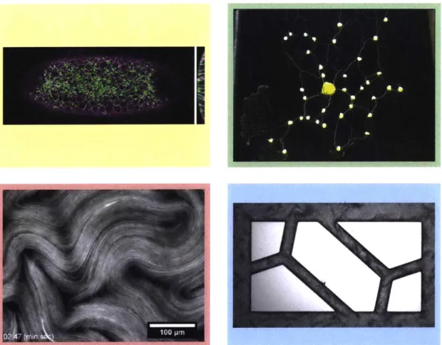
1-1 Active driving interacts with networks in diverse biological systems. (a) In Drosophila embryos, networks of ATP-driven myosin motors (fluo-rescently labeled in green) couple to the cell boundaries (magenta) to control tissue folding

[33].

(b) The slime mold Physarum polycephalum

(yellow) can form complex optimized transport networks to connect food sources like the oat flakes (white dots) shown. Here, the food was placed in roughly the pattern of population centers around Tokyo. The organism's final state is reminiscent of the human-designed rail system [131]. (c) Microtubules and kinesin motors like these from the Dogic lab can be confined to channels where they drive coherent shape-dependent flows

[1471.

(d) Our theoretical work models most closely confined suspensions of swimming microbes. In this picture, from pre-liminary experiments by the Kantsler lab, sperm cells are confined to a network of channels in a microfluidic chamber with barriers (light gray

polygons). . . . . 28

2-1 Stochastic cycle selection in two elementary graphs. (a) Flux-time traces from Eq. 2.4 for each of the three edges in the graph shown, signed according to the edges' arrows, with three different temporary configurations highlighted as indicated by (i)-(iii). A = 2.5, p = 25,

/-- = 0.05. (b) Same as (a), but with an additional edge in the graph.

States are more stable with even-degree vertices, since flux conserving flows are possible with all edges flowing. . . . . 32

(12)

2-2 Noise and activity cause stochastic cycle selection. (a-c) Flux-time traces (b) for each edge of the complete graph on four vertices, K4.

Edge orientations are as in (a). The sub-diagrams in (c) (i-iv) exemplify the flow state in the corresponding regions of the trace. Parameters

A = 2.5, t = 25, 0-1 = 0.05. (d-f) As in (a-c), but for the generalized

Petersen graph P3,1. The same switching behavior results, but now

with more cycle states. (g) Survival function S(t) = P(T > t) of the transition waiting time T for an edge in K4, at regularly-spaced values

of A in 2 < A ( 3 with p = 25, 0-1 = 0.05. Log-scaled vertical; straight

lines imply an exponential distribution at large t. Inset: S(t) at small t with log-scaled vertical, showing non-exponential behavior. (h,i) Slow and fast edge transition rates in K4, with parameters as in (g). Circles

are from fitting T to a mixture of two exponential distributions, lines show best-fit theoretical rates k oc A exp(-3AH) with AH calculated for transitions between 3- and 4-cycles.

(j)

Transition rate k =

(T)-for each set of equivalent edges in P3,1, as per the key, as a function

of A, with t = 25, /- 1 = 0.05. Log-scaled vertical shows exponential

dependence on A. ... ... 38

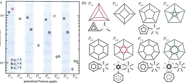
2-3 Transition rates in highly symmetric graphs are determined by cycle structure. (a) Transition rate for edges in the first eight generalized Petersen graphs with A = 2.5, i = 25, -1 = 0.05. The rate was

determined for each edge, then averaged within classes of equivalent edges. Symbols denote the rate for each class, categorized by e-girth g, as in the key. The range of computed rates within each class is smaller than the symbols. (b) The graphs in (a) with their edge equivalence classes when more than one exists. Edges colors denote g, as in (a). Observe that identical e-girth does not imply equivalence of edges. . 43

(13)

2-4 Cycle structure determines edge transition rates in asymmetric graphs. (a) Transition rate for each edge in 20 random asymmetric bridgeless cubic graphs on 21 edges. Markers denote e-girth ge as per the key in (c). A = 2.5, [t = 25, A- 1 = _{0.05. (b) One of the graphs in (a),} corresponding to the marked column (*). Edges colored and labelled according to g.. All 20 graphs are shown in Fig. 2-5. (c) Transition rates k from (a) binned by girth-weighted rate Rg, using best-fit value

a = 1.31, with markers denoting ge as per the key. Horizontal error

bars are range of marker position over 95% confidence interval in a, vertical error bars are 1 standard deviation in k within each group. Solid line is best fit k = -yRg, dashed lines are 95% prediction intervals on k w ith a fixed. . . . . 45 2-5 The 20 non-isomorphic asymmetric cubic graphs in Fig. 2-4. Edges are

colored according to e-girth as indicated in graph 1 and in Fig. 2-4. Graph 19 is that illustrated in Fig. 2-4b. All planar graphs (2, 3, 5, 6, 7, 12, 16 and 19) are shown in a planar embedding. . . . . 46 2-6 Constructing a cycle basis for P4,1. (a) A planar embedding of P4,1, with

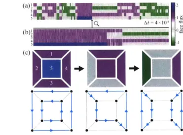
edges numbered and oriented as shown. (b) The dual of the embedding in (a), with dual graph vertices (original graph faces) numbered as shown. Edge orientations depend on those chosen in (a), as described in the text. Vertex 6 and its incident edges, highlighted, correspond to the external face whose flux is fixed at zero. . . . . 50 2-7 Incompressible flow on planar graphs can be represented using a

face-based cycle basis. (a) Flux-time traces for flow about each of the internal faces of P4,1, as labelled in (c), from Eq. (2.11) with A = 2.5,

0-1 = 0.05. (b) Zoom of trace showing a transition between two 8-cycles, which are global minima, via a 6-cycle. (c) Distinct state configurations in (b) of face fluxes (upper) and corresponding edge flow s (low er). . . . . 52

(14)

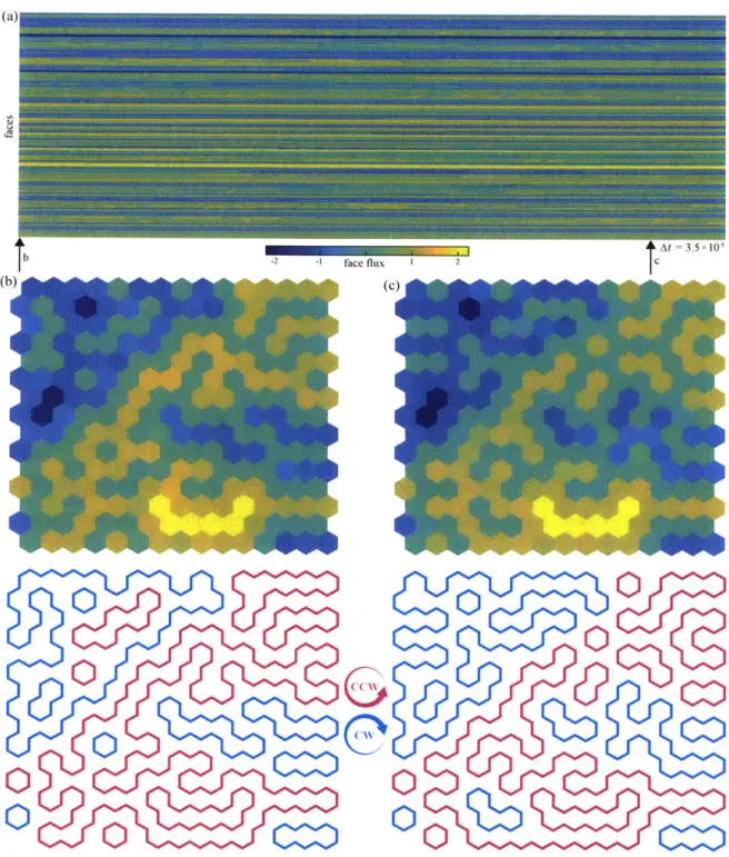
2-8 Incompressible flow on a 15 x 15 hexagonal lattice using the face cycle basis. (a) Plot of flux values over time for each face in an integration on the 15 x 15 lattice, at A = 2.5, p = 25, /#' = 0.05. (b,c) Configurations of the face fluxes at the times marked in (a), along with the cycle configurations they represent. Cycles are colored according to their orientation clockwise (cyan) or counterclockwise (magenta). Faces are ordered in (a) column-wise from bottom-left to top-right of the lattice. 53 2-9 Empirical probability distributions of e-girth determined from ten graph

realizations each from four random 1000-vertex graph ensembles: (a) fixed degree 3, i.e. cubic; (b) uniform with 1500 edges; (c) 'scale free' Barabdsi-Albert with a degree k = 2 vertex added at every step; and

(d) 'small world' Watts-Strogatz with rewiring probability p = 0.5 and

mean degree k = 4. The pseudo-real-life networks of (c) and (d) exhibit distributions with far more small e-girth edges than the more generic

random graphs in (a) and (b). . . . . 55

3-1 Our active network model exhibits behavior similar to the topological edge modes of Ref.

[1241.

(a) A discretized version of the Lieb lat-tice considered in Ref. [124]. Edges shared by adjacent 8-cycles have weight we = 2 to account for the additional width of the correspond-ing channels. The most stable flow on this network consists of a lat-tice of counter-rotating cycles, in which both the active friction term

g(p, qe/ ) and the pressure variations p, are everywhere zero. (b)

This lattice has modes confined to the edges of the domain, allowing sound waves to propagate and decay without scattering into the bulk (cf. discussion in App. I.B of Ref. [1241); one such mode is pictured. Simulations started in this mode as a perturbation to the most stable flow pattern do not cause density changes in the center. The network model allows study of such phenomena without resorting to full scale

(15)

3-2 Activity can select a single dominant oscillation mode on hierarchically weighted networks. (a) The edges in the graph simulated in (b) and (c) are given weights decreasing exponentially with their distance from the central red path. (b) Oscillations in pressure and flux develop primar-ily along the central high-weight path. (c) Edge fluxes

#e

settle into steady synchronized oscillations as exemplified for two edges indicated in (b), one on (017) and one off (#59) the path. (d) Plotting the time-dependent amplitude of each analytically-determined flow eigenmode confirms selection of a single oscillatory mode. The ten modes with the highest average amplitude in this simulation run are pictured; the marked top two rows are oscillatory modes, while the remaining rows are cyclic modes. See Fig. 3-3 for all modes. Simulation parameters are E=0.1,

p=

1, andD= 104 . . . . . 67

3-3 Including all of the modes from the simulation in Fig. 3-2 shows clear single mode selection on this weighted network. Edges a distance d from the central red path were given weight e-. Modes are ordered by frequency from high (top) to low (bottom); the last thirty modes, marked in red, are cycles. The modes pictured in Fig. 3-2 are marked in b lack . . . . . 68

3-4 Steady state amplitudes Ai as a function of activity p for the tree pictured undergo a Hopf bifurcation as p crosses 0. Dots are long-time root-mean-square amplitudes from simulations started in each mode; lines are numerical solutions of Eq. (3.20). Mode A2 is too unstable

to reliably observe in simulations, so it is omitted. For ya < 0, all amplitudes go to zero in simulations; the dot included in that region is at [ = -1 where the friction is purely passive. Some deviations between simulation and analytics are expected because the simulations do not use the Rayleigh friction approximation and c k 0. Parameters

(16)

3-5 First order perturbation theory accurately predicts the stable states on small trees. (a) A five vertex tree possessing four nontrivial modes, as illustrated. (b) On the tree in (a), mode amplitudes settle into one of two stable stationary states, as seen in simulations for three different initial conditions. Modes are ordered by frequency from high (top) to low (bottom). (c) Simulated mode trajectories (rainbow) in (b) match analytic predictions (blue streamlines) in the subspaces of activated modes. There are three possible arrangements of nonzero critical points in each 2D subspace: a saddle point on one axis and a stable node on the other axis (left), a stable node on each axis and a saddle point in the middle (center), or a saddle point on each axis and a stable node in the middle (right). Higher order effects cause both the convergence to a point with A2 > 0 in the left and middle plots

and the oscillations in the trajectories. Parameters used are C = 0.5,

(17)

3-6 States on larger trees possess surprisingly few active modes, which can be inferred from time series with non-zero noise. (a) The mean num-ber of stationary states of Eq. (3.13) grows exponentially with edges

E as 1.7 7E (E 4/5 (solid orange line), close to the upper bound of

2E states (dashed black line), while the mean number of stable states grows as 1.2 (2E)1/4 (solid blue line). We counted states on all nonisomorphic trees with E < 14 edges (filled circles) and on a ran-dom sample of ~ 175 trees per point for 15 < E < 24 (open circles). Averages are over trees with a fixed number of edges. (b) As E in-creases, both the mean and the variance of the distribution of trees with each number of stable states increase rapidly. (c) Distribution of the average number of modes active in a stable state. The mean over trees scales like 0.26E ~ E/4 (solid line), significantly below E/2 expected if modes were selected randomly. (d) Two example trees in-dicated in (a-c) by the corresponding colored symbols. Stable states on paths (x) always only activate one mode; complex trees

(+)

have more modes active. (e) Noisy networks (D > 0) transition stochasti-cally between stable states, exemplified by an amplitude-time trace for the tree shown. Modes are ordered by frequency from high (top) to low (bottom). Simulation parameters are c = 0.5, p = 1, D = 5 x 10-3. (f) States found by vbFRET from simulations on the tree in (e). The second, first, and fifth columns are states seen in (e), indicated by the colored bars above. (g) States predicted by Eq. (3.13) for the tree in (e). The first five states in (f) match those in (g); the sixth column in (f) is likely a transient combination of analytically stable states. . . . 78

(18)

3-7 Slow global oscillations emerge from the fast active dynamics. (a) First order considerations fix a constant mean flow energy; higher order effects cause significant slow oscillations about that mean. Simulation parameters were yu = 1, E = 0.5, and D = 0; the tree used is inset. (b) The mode amplitudes A2 and A3, like the energy, oscillate much

more slowly than the harmonic oscillations of f2 and

f3.

All other mode amplitudes (unlabelled traces) are close to zero. (c) Frequency spectra of the two active modes and the energy H for the simulation in (a) and (b). The energy oscillates due to higher-order interactions between modes at frequencies that are linear combinations of active

mode frequencies, not the harmonic frequencies alone (dashed lines). 81

3-8 Activity causes depth-dependent separation of time scales on a large tree. (a) Most pressure variation occurs near the leaves on large binary trees. (b) The tree in (a) develops an activity-driven steady state with slow oscillations in the center and fast oscillations near the edges, as illustrated by the flux 0, on the three edges labelled in (a). (c) Unnor-malized correlations between the Fourier transforms of the flux through the edges of the tree in (a), with phases ignored. Colors indicate the tree level of the tail vertex of the edge. There are strong correlations within each level and between neighboring levels, but low correlations for edges in widely-separated levels. (d) Frequency spectra of each tree level, computed by taking Fourier transforms of the edge fluxes as in (c) and averaging the magnitudes across all edges at each level. A distinct primary oscillation frequency for each level can be seen, which increases with distance from the tree center. Simulation parameters in all panels are E = 0.5, p = 1, and D = 10-3. (e-h) While adding edges in the center leads to steady flow on cycles there, frequency still increases with distance from the center in the outer, tree-like sections. 86

(19)

3-9 Lower energy modes transition more often for the graph in Fig. 3-6. Modes are ordered by frequency from high (top) to low (bottom). Simulation parameters are 6 = 0.5, p = 1, D = 5 x 10-3, identical to those in Fig. 3-6. Note that rows 7 and 8, the two modes that switch on and off most, are degenerate. . . . . 87

3-10 States on graphs with cycles, like the one shown, tend to be more stable. Modes are ordered by frequency from high (top) to low (bottom). Note that the eight modes at the bottom, which are the only ones active in the lower half of the trace, are all cycles. Simulation parameters are E = 0.5, p = 1, D = 5 x 10-3. . . . . 88

3-11 The emergence of an activity-driven spectral band gap is exhibited by a simulation on a 14-vertex path with (a) all weights equal to 1 and (b) alternating vertex weights 1 and 5. Modes are ordered by frequency from high (top) to low (bottom). Note that in (b) the central n = 7 mode is always active and the low energy states on the right half of the plot are significantly more suppressed than they ever are in (a). The qualitative difference is due to the presence of vertices with unequal weights, not the overall scale of the vertex weights; changing vertex weights uniformly is equivalent to rescaling other parameters. Parameters are p = 1.2, D = 5 x 10--3, and E = 0.5. Both simulations

(20)

4-1 Designing networks from spectra. (a), Schematic of DBG network construction. Given a spectrum of eigenvalues distributed in two (or more) groups, we build a graph with non-negative edge weights that realizes this spectrum exactly (1). Sparsification of this complete DBG network with the Spielman-Srivastava [125] algorithm (2) yields a new network with wider eigenvalue distributions and a smaller gap (3). (b), Example graphs used in applications below: Starting from a DBG graph on 200 vertices with 100 eigenvalues set to i.i.d. K(5, 0.25) and 99 set to i.i.d. A(20, 0.25) (left), sparsification with e = 0.5 creates a new graph (top) with the number of edges reduced from 19900 to 3758. As a control, we also compare to a gapless random graph (bottom) with 362 edges and the same weighted vertex degrees as the original DBG graph. (c), The eigenvalues for the graphs in (b). The mode on the complete DBG network with the k-th largest nonzero eigenvalue is supported on the first k

+1

vertices, counted counterclockwise from the top red vertex, and highly localized on vertex k

+1,

which is colored to match in (b). Grey lines indicate the borders of the unstable region for the Swift-Hohenberg model with the parameters used in Fig. 4-3. (d), Sparsified networks retain a significant gap even for relatively large C. Each point shows the mean number of edges and gap size at fixed E

between 1 (left) and 0.01 (right), starting from a graph on 200 vertices designed to have 100 x eigenvalue 5 and 99 x eigenvalue 20. The solid curve shows the worst-case gap estimate, reduction by a factor 1 - 5C.

Sample size is 1000 for c > 0.1 and 300 for 6 < 0.1. Error bars are 1 standard deviation; horizontal error bars are smaller than the marker size . . . . . 9 7

(21)

4-2 DBG networks lead to staggered synchronization and chimeras.

(a-f), In the Kuramoto model with a = 0, the complete (first row) and

sparsified (second row) graphs synchronize much faster than the ran-dom graph (third row). For the complete graph the gap affects the rate of synchronization, with highly-connected vertices synchronizing faster (a), while on the sparsified graph the gap is only visible in the mode basis (e). (g-i), Weak chimera states appear when a = 1. Both the complete (g) and sparsified (h) graphs have two dominant groups of phase-locked oscillators, with the complete graph more fully synchro-nized. Dynamics on the random graph (i) are much less coherent. Solid black lines indicate the predicted approximate frequency difference for a network with two distinct eigenvalues, 5 and 20. (j-1), Order parame-ter r = I ea I for the simulations in (g-i) for the strongly-connected vertices (red), weakly-connected vertices (teal), and all vertices (gray). 102

4-3 Generic suppression of pattern formation with a designed discrete band gap. (a), Pattern formation in the Swift-Hohenberg system is com-pletely suppressed by constructing a gap around the range where eigen-values would be unstable (Fig. 4-1c). (b), On a sparsified graph that has a few eigenvalues just within the unstable region, some modes set-tle at small nonzero values. (c), On the random graph many more eigenvalues are well within the unstable region and the corresponding modes settle at larger amplitudes. Inset graphs show the final steady state on each graph; the size of vertices corresponds to 101. All sim-ulations used identical initial conditions ai - )A(0, 1) and parameters

(22)

4-4 Controlling pattern formation with a designed discrete band gap. (a) Instead of placing a gap in the spectrum around the unstable pattern-forming range, as in Fig. 4-3, we deliberately place particular eigenval-ues in the middle of that range corresponding to eigenvectors localised on a desired pattern. (b) From random initial conditions, the system settles into a state where only the chosen modes have nonnegligible am-plitudes. (c-e) Time series of pattern evolution on a designed network, with vertices colored according to the stability of the mode localized there as in (a). The size of the vertices indicates 101. (c) The encoded pattern is not obvious from either the designed network or the random initial conditions. (d) By time t = 0.07 the stable modes have nearly all vanished. (e) The steady state reveals the eigenmode-designed pat-tern. Because the modes are highly localized, selecting a set of modes to activate is approximately equivalent to selecting a set of vertices to activate. Thus we can encode an arbitrary pattern as the steady state. Depending on initial conditions, the system may settle into other sta-ble states with slight variations in the vertex activations; the pattern is always identifiable and often as clear as shown. The parameters a = 90, D, = -20, and D2 = 1 are identical to those in Fig. 4-3; the

tuning parameters to control pattern formation are only the network edge w eights. . . . . 108

(23)

4-5 Localization on a DBG quantum network. (a-c), When the wavefunc-tion in the Gross-Pitaevskii model of Eq. (4.20) is initialized at a weakly connected vertex with low kinetic energy, localization or delocalization (indicated by high or low potential energy, respectively) is controlled by the interplay between the graph spectrum and the rate of potential energy loss g. The random graph (purple) always delocalizes, due to its dense spectrum. However, while the sparsified graph (yellow) can de-localize for low g (a) and high g (c), again due to available eigenmodes, intermediate g (b) places the range of allowed modes inside the spec-tral gap, preventing delocalization. The complete graph (blue) always inhibits spreading due to the extreme localization of its eigenvectors. 111 4-6 Designed spectra on a discrete network are preserved when extended

periodically in one dimension. (a) We extend a finite network to an infinite one by rewiring a subset of the edges to cross between adjacent copies of the original network. Here, we take the network with the spectrum in (b) and rewired the edge between vertices

j

and k if Ik

-jI

> n/2. This rewires roughly one quarter of the edges. (b) One unit cell in (a) would have a discrete spectrum with A = 21-j. (c) Most of the eigenvalue bands do not change significantly with q, so the density of states consists of 21 sharp peaks with low- or zero-density regions between. (d) The same construction as in (a) can be repeated for any spectrum; this is the result for a gapped network. (e) One unit cell in (d) would have a gapped spectrum, with 10 eigenvalues equal to 20 and 10 equal to 5, in addition to the always-present zero eigenvalue. (f) Again, most of the eigenvalue bands are roughly constant, even though the eigenvectors do depend strongly on q. The gap in the middle of the spectrum is nearly perfectly preserved; a small gap remains between the bottom two bands. Note the log scale on both density of states p lots. . . . . 113

(24)

(25)

Chapter 1 Introduction

This thesis will explore two related topics in network theory. For the first two chap-ters, we will study active flows, investigating the nonequilibrium mode selection prin-ciples [43, 45] governing their dynamics in the network setting. The tools from the active flow chapters are in fact of much more general interest. In particular, one mathematical object called the graph Laplacian plays a critical role in problems across mathematics and physics. Motivated by this broad relevance, we will show in the last chapter how to construct networks with exactly specified Laplacian spectra.

1.1 Active flows

Classical fluid dynamics deals with externally-imposed driving forces such as gravity or applied pressure gradients. These passive fluids dissipate energy through viscosity, but do not generate it. Biological systems may act very differently, producing energy at a very small scale, perhaps individual swimming bacteria, and propagating the energy upwards to drive larger flows. Often, the flows occur within an intricate network structure (Fig. 1-1). These biological flow networks, such as capillaries

[51],

leaf veins 67], and slime molds [2], use an evolved topology or active remodeling to achieve near-optimal transport when diffusion is ineffectual or inappropriate [10, 39,

67, 95, 131].

(26)

information currents along physical or virtual links between interacting nodes, as in neural networks [31], biochemical interactions [65], epidemics [103], and traffic flow

[50].

The ability to vary the flow topology gives network-based dynamics a rich

phenomenology distinct from that of equivalent continuum models

[96].

Identical

local rules can invoke dramatically different global dynamical behaviors when node connectivities change from nearest-neighbor interactions to the broad distributions seen in many networks [1, 12, 21, 141]. Certain classes of interacting networks are now sufficiently well understood to be able to exploit their topology for the control of input-output relations [90, 97], as exemplified by microfluidic logic gates [104, 109]. However, when matter or information flow through a noisy network is not merely pas-sive but actively driven by non-equilibrium constituents [2], as in maze-solving slime molds [95], there are no overarching dynamical self-organization principles known. In such an active network, noise and flow may conspire to produce behavior radically dif-ferent from that of a classical forced network. This raises the general question of how path selection and flow statistics in an active flow network depend on its interaction topology.

Flow networks can be viewed as approximations of a complex physical environ-ment, using nodes and links to model intricate geometric constraints [41, 42, 148]. These constraints can profoundly affect matter transport [17, 47, 63, 92], particu-larly for active systems [44, 85, 137] where geometric confinement can enforce highly ordered collective dynamics [24, 30, 48, 80, 102, 104, 110, 132, 144, 146, 150]. In sym-metric geometries like discs and channels, active flows can often be effectively captured

by a single variable 0(t), such as angular velocity [143, 144] or net flux

11501,

that

tends to adopt one of two preferred states o. External or intrinsic fluctuations can cause

#(t)

to diffuse in the vicinity of, say, - 00 and may occasionally trigger a

fast transition to

#o

and vice versa [143, 150]. Geometrically coupling together many such confined units then results in a lattice field theory, reducing a non-equilibrium active medium to a discrete set of variables obeying pseudo-equilibrium physics, as was recently demonstrated for a lattice of bacterial vortices [143].

(27)

an incompressible active medium flowing in an arbitrary network of narrow channels. By connecting concepts from lattice field theory, graph theory, and transition rate theory we can understand how topology controls dynamics for this actively driven network flow. Our combined theoretical and numerical analysis identifies symmetry-based rules that make it possible to classify and predict the selection statistics of complex flow cycles from the network topology. The conceptual framework devel-oped is applicable to a broad class of non-biological far-from-equilibrium networks, including actively controlled information flows, and establishes a new correspondence between active flow networks and generalized ice-type models. The content of chap-ter 2 was published in the Proceedings of the National Academy of Sciences

[145].

In Chapter 3, we extend to the compressible case where variations in local den-sity or volume are dynamically relevant. Using perturbation theory, we systemati-cally predict the stationary states of noisy networks and find good agreement with a Bayesian state estimation based on a hidden Markov model applied to simulated time series data. Our results suggest that the macroscopic response of active network structures, from actomyosin force networks to cytoplasmic flows, can be dominated by a significantly reduced number of modes, in contrast to energy equipartition in thermal equilibrium. The model is also well-suited to study topological sound modes and spectral band gaps in active matter. This work appeared in Physical Review

Letters 146].

1.2 Graph Laplacians

Complex real-world phenomena across a wide range of scales, from aviation

[25]

and internet traffic [1511 to electronic

[36]

and gene regulatory

[83]

circuits, can be effi-ciently described through active and passive network models encoded with weighted graphs. Their dynamics are often essentially determined by the associated graph Laplacian, which we introduce here. A weighted simple graph G is defined by its vertex set V, edge set 9 containing unordered pairs of distinct vertices (u, v), and corresponding edge weights w.. We consider the case with real, nonnegative weights

(28)

Figure 1-1: Active driving interacts with networks in diverse biological systems. (a) In Drosophila embryos, networks of ATP-driven myosin motors (fluorescently labeled in green) couple to the cell boundaries (magenta) to control tissue folding

[33].

(b) The slime mold Physarum polycephalum (yellow) can form complex optimized transport networks to connect food sources like the oat flakes (white dots) shown. Here, the food was placed in roughly the pattern of population centers around Tokyo. The organism's final state is reminiscent of the human-designed rail system [131]. (c) Microtubules and kinesin motors like these from the Dogic lab can be confined to channels where they drive coherent shape-dependent flows [1471. (d) Our theoretical work models most closely confined suspensions of swimming microbes. In this picture, from preliminary experiments by the Kantsler lab, sperm cells are confined to a network of channels in a microfluidic chamber with barriers (light gray polygons).

(29)

'wUV > 0 and set wu, = 0 if there is no edge between u and v. The Laplacian of G

is the matrix whose off-diagonal elements are the negatives of the edge weights and whose diagonal elements are the weighted vertex degrees. That is, Lu, = -wu, for

u v and LUU = E' wUV

The Laplacian matrix occurs naturally in a wide range of physical systems. Up to a sign, it is the discrete analog of the continuous Laplacian: where V2 _appears

in continuous models, -L typically appears in the discrete version of the model. For example, the ubiquitous nearest-neighbour finite difference approximation to V2

arises as the graph Laplacian of a square lattice

162].

In Chapters 2 and 3 we will work with the discrete gradient operator Ve, which with weighted edges equals - /w if there is an edge from u to v, wU, if there is an edge from v to u, and zero otherwise. For any arbitrary orientation of G, the Laplacian is equal to the gradient times its

transpose: L U = E, VueVLT. The singular value decomposition of Vu, which will

feature prominently in Chapter 3, is then the eigendecomposition of L.

The simplest physical examples of network Laplacians come from spring systems and discrete random walks. If a set of identical masses moving in one dimension are coupled by springs with stiffness wuv between masses u and u, the force on mass u is exactly - EZ Luvz = ZE wuv(x - xu). Here xu is the coordinate of the uth mass. The mechanics then decouple into n = IVI oscillation modes corresponding to the eigenvectors of L, with the eigenvalues as squared frequencies.

Similarly, if a particle follows a random walk on a network, traveling from node u to node v with rate wuv (so the probability flow from u to v is the probability pu of being in state u times the rate), then the probability distribution evolves in time according to

=p _dt _{V u}wUVPU + _viuE war PV V LUVpo.(11

The solution again comes from the eigendecomposition of L: the eigenvalues deter-mine the diffusion rate and the rate of decay to the stationary distribution.

It is natural, then, to ask whether we can control these eigenvalues. By design-ing the network appropriately, what spectra can we construct? There are two clear

(30)

constraints. First, the rows and columns of L sum to zero, implying that 1, the vec-tor of all ones, is an eigenvecvec-tor with eigenvalue zero. This eigenvecvec-tor corresponds to the stationary distribution for the random walk, rigid translation for the spring system, and a constant pressure shift for flow networks. Moreover, the remaining eigenvalues must be nonnegative by the Gershgorin circle theorem [27]. We will see in Chapter 4 that these are the only two restrictions for weighted networks, and that by explicitly constructing networks to have particular spectra we can control a wide variety of classic physical models, including Kuramoto-type coupled oscillators, Swift-Hohenberg pattern formation, and quantum Gross-Pitaevskii dynamics.

(31)

Chapter 2 Incompressible flow networks

In this chapter we introduce the active network model in the incompressible setting.1 Combining concepts from transition rate theory and graph theory, we show how the competition among incompressibility, noise, and spontaneous flow can trigger stochastic switching between states comprising cycles of flowing edges separated by acyclic sets of non-flowing edges. As a main result, we find that the state transition rates for individual edges can be related to one another via the cycle structure of the underlying network, yielding a topological heuristic for predicting these rates in arbitrary networks. We conclude by establishing a mapping between incompressible active flow networks and generalized ice-type or loop models [14, 16, 721.

2.1 Model

2.1.1 Lattice

q56

field theory for active flow networks

Our network is a set of vertices v E V connected by edges e

E

S, forming an undirected loop-free graph G. (We use graph theoretic terminology throughout, where a loop is a single self-adjacent edge and a cycle is a closed vertex-disjoint walk.) To describe signed flux, we construct the directed graph d by assigning an arbitrary orientation

'This work was published in the following paper:

Francis G. Woodhouse, Aden Forrow, Joanna B. Fawcett, and J6rn Dunkel. Stochastic cycle selection in active flow networks Proc. Natl. Acad. Sci. U.S.A., 113(29):8200-8205, 2016.

(32)

(a) At= 1000 (b ₎ *0 i ii -II

21.

21

_{At~ 1000}

Figure 2-1: Stochastic cycle selection in two elementary graphs. (a) Flux-time traces from Eq. 2.4 for each of the three edges in the graph shown, signed according to the edges' arrows, with three different temporary configurations highlighted as indicated

by (i)-(iii). A = 2.5, p = 25, 0--' = 0.05. (b) Same as (a), but with an additional edge in the graph. States are more stable with even-degree vertices, since flux conserving flows are possible with all edges flowing.

to each edge. Now, let

#,

be the flux along edge e, where 4

e > 0 denotes flow

in the direction of the orientation of e in d and qe < 0 denotes the opposite. To model typical active matter behavior 180, 143, 144, 146J, we assume that fluxes either spontaneously polarize into flow states

#,

~ +1 or adopt some other non-flowing mode qe ~ 0. We formalize this by imposing a bistable potential V(#e) on each flux variable. The typical symmetric, bistable potential is the quartic V4(0) = - 2+

#04.

However, we use the sixth-order form V(O) = V₆(0) - - 94 + 106. This form, of

higher order than in a typical Landau theory, ensures that incompressible potential minima are polarized flows with every

#e

in the set

{-1,

0, +1}, rather than the continuum of fractional flow states that a typical

#4

potential would yield.

Incompressibility, appropriate to dense bacterial suspensions or active liquid crys-tals, is imposed as follows. The net flux into vertex v is EeC Vve~e, where the discrete negative gradient operator V = (Vve) is the IVI x 191 incidence matrix of G such that Vve is -1 if e is directed out of v, +1 if e is directed into v, and 0 if e is not incident to v

[53].

Exact incompressibility corresponds to the constraint V(D = 0 on

(33)

the global flow configuration D = (0e) E R I. To allow for small fluctuations,

model-ing variability in the microscopic flow structure, we apply this as a soft constraint via

an interaction potential oc IV(D2_{. The total energy H(z) of the active flow network}

then reads

H(1) = A V(#e) + }PIV(If2_, _(2.1)

eEE

with coupling constants A and y.

To see why V₄(0) has the undesirable symmetry mentioned above, consider the

elementary (though not simple!) two-vertex, three-edge graph in Fig. 2-la. Here the energy is

H(0

1, q52, 53)= A[V(# 1) + V(02) + V(03)] + P(01 + #2 + 33)2.

In the limit p/A

>>

1, the flow is incompressible, so we can substitute03 = -#1 - 02

to obtain a reduced energy H(#1,

#

2) = AN(# 1,

#

2), where, assuming a symmetric

potential V(O),

W((i, #2) = V(01) + V(02) + V(01 + #2).

Local minima of R then yield metastable states of the system, independent of A. Consider the case V = V4. Then R factorizes as

2- = f(1, q2)[f (#1, 02) -2],

where f(#1,

#2)

=1# + q102 +

#2.

Thus V- = 0 implies (f - 1)Vf = 0, so either

f

= 1 or q1 =

#2

= 0. The latter is a local maximum, so our minima are the

solutions of

#2

+ 10#2 +

#2

= 1. But these solutions form an ellipse in the (#1,

#2)

plane, implying a continuous U(1)-symmetric set of fixed points. In other words, with V = V4, mixed states such as

( ,

3, - ) are equally preferable to unit-flux

(34)

the six states (q 1, $2) = ( I, 0), (0, 1), ( 1, -1), which is the phenomenology we

are interested in. Based on simulations, these results carry over to more complicated networks, though we do not prove so here; V4 typically allows mixed states while V6

selects unit fluxes.

The energy in Eq. (2.1) is comparable to that of a lattice spin field theory, but with interactions given by higher-dimensional quadratic forms akin to a spin theory on the vertices of a hypergraph. Suppose we switch to a typical vertex-based picture, where fluxes

#,

on edges e in G are now spins 4

'i on vertices i in an interaction graph

B. A scalar lattice spin theory then has Hamiltonian

Hspi = Aj V(V/i) + It ((bi ij 0j)2, (2.2)

i {i,j}

where in the sum over adjacent spins

{i,

j}

in E, the sign ij is + or - according to whether the interaction between i and j is antiferromagnetic or ferromagnetic, respec-tively. In our theory, however, multiple spins are permitted inside each interaction term according to the degree of each vertex in G. For instance, on a cubic graph, the energy (2.1) is equivalent to

H = AZV(Vi) + 'A E ()i ij )j jk /k )2 (2.3)

i {i,j,k}

where the interaction is now a sum over interacting triples of spins, one term for each vertex in G, with pairwise signs being - or

+

according to whether the corresponding edges in C are oriented head-to-tail or not at the vertex. Thus we have essentially defined a theory on an interaction hypergraph E, with Eq. (2.2) being the special case where E is a graph: while Eq. (2.2) has two types of interaction edge-antiferro- and ferromagnetic-between two spins, the general theory has 2n-1 types of interaction

(35)

2.1.2 Network dynamics

Appealing to recent results showing that bacterial vortex lattices obey equilibrium-like physics

[143],

we impose that 4 obeys the overdamped Langevin equation

5H

d = H dt + 2/3-'dW,, (2.4)

64D

with Wt an JEJ-dimensional vector of uncorrelated Wiener processes and 3 the inverse temperature. We choose additive noise for mathematical simplicity and because we focus on the effect of the active driving; plausibly, more detailed physical modeling could lead to a different stochastic term potentially depending on 1. This would change the quantitative results of this chapter and Chapter 3, for example the cal-culation of transition rates, but broad qualitative features like the selection of stable flow states will remain.

The stochastic dynamical system in Eq. (2.4) has a Boltzmann stationary distri-bution xc e-H. The components of the energy gradient 6H/& in Eq. (2.4) are

(

) _{-A053(1 _}_{q2) +}_ii(VT _V4)e.

(2.5)

641 e *

25

VTV is the discrete Laplacian operator on edges, which is of opposite sign to the

continuous Laplacian V2 by convention. Remember that the vertex Laplacian defined

in Chapter 1 is equal to VVT; the edge Laplacian is a related but distinct operator. The last term in Eq. (2.5) arises in an otherwise equivalent fashion to how a bending energy IV012 yields a diffusive term V2V in a continuous field theory. On its own,

this term damps non-cyclic components of the flow while leaving cyclic components untouched; these components' amplitudes would then undergo independent Brownian walks were they not constrained by the

#

6 component of V. This process results in a long-term state dominated by a weighted sum of cycles of the graph, as we now describe.

As in the derivation of the incompressible limit (see section 2.3.1 below), by anal-ogy with a spectral decomposition for the diffusion equation, we decompose 4 into a

(36)

sum =

fT

h _{1! over an orthonormal eigenbasis T3 of the edge Laplacian}VTV, where

'F'= (04) has eigenvalue v4 > 0. If A is set to zero, the components

fi

then obey

dfi = _{-wvi fidt + f2/-} 1_dWi,1,

after combining independent noise terms. Thus modes with vi > 0 are damped by the diffusivity it while modes with vi = 0 are only subject to noise-induced fluctuations. The non-zero modes' amplitudes follow Ornstein-Uhlenbeck processes and therefore have mean zero and variance

(/pu')

1 _{as t}_- _oc,_{whereas, because of the absence of}

damping, the zero modes' amplitudes follow simple Brownian processes and so have variance 2/3-1t.

With these dynamics for any A, all loops in G, i.e., edges of the form (w, w) from one vertex to itself, will decouple from the dynamics of the rest of G. Consider a loop edge f E S incident to a vertex w E V. Then V is defined such that Vwe = 0 (consistent with

#e

contributing zero to the net flux at w, since flow in along f always equals flow out along f). Therefore, using summation convention, Vvee is independent of Oj for all v E V, which implies aH/#eq is independent of Of for all e and thus Of decouples. Furthermore, (VTVII)f = VfVvOeqe = 0, so do =

-AV'(0e)dt+ 23-IdWt,t, meaning Of behaves as a non-interacting Brownian particle

in the potential V(#t). The remaining non-loop edges follow Eq. (2.4) exactly as they would on the subgraph of G with all loops removed.

Altogether, the preceding paragraphs mean that the interesting behavior is con-fined to flows around interacting cycles. We now characterize the behavior of this model on a variety of forms of underlying graph G. For clarity, in addition to our prior assumption that G is loop-free (which simplifies definitions and is unimpor-tant dynamically since loops decouple), we will focus on connected, simple graphs G, though multiple edges are not excluded per se (Fig. 2-1). In what follows, we work in the near-incompressible regime p

>

A before discussing the strictly incompressible

(37)

2.2 Results

2.2.1 Stochastic cycle selection

The combination of energy minimization and noise leads to stochastic cycle selection. A local energy minimum comprises a maximal edge-disjoint union of unit-flux cycles: edge fluxes seek to be at 1 if possible subject to there being zero net flux at every vertex, leading to states where the non-flowing edges contain no cycles (that is, they form a forest, or a union of trees). However, noise renders these states only metastable and induces random switches between them. Figure 2-2a-f depicts flow on the 4-vertex complete graph K4 (Fig. 2-2a-c) and the generalized Petersen graph P3,1 (Fig.

2-2d-f)-the tetrahedron and triangular prism, respectively-where we have integrated Eq. (2.4) to yield flux-time traces of each edge. The coordinated switching of edges between states of mean flux at -1, 0 and

+1

leads to random transitions between cyclic states, as illustrated. Note that the more flowing edges a state has, the lower its energy and therefore the longer-lived that state will be; thus in K₄, for example,

4-cycles, which are global minima, persist longer than 3-cycles (Fig. 2-2b,c).

A graph possessing an Eulerian cycle-a non-repeating tour of all edges starting and ending at one vertex, which exists if and only if all vertices are of even degree-has global energy minima with all edges flowing. By contrast, a graph possessing many vertices of odd degree will have minimum energy states with non-flowing edges, because edges flowing into and out of such a vertex pair up to leave an odd number of 0-flow edges. Such 'odd' networks are particularly interesting dynamically as they are more susceptible to noise-induced state switches than graphs with even degree vertices. This susceptibility is exemplified by the small graphs in Fig. 2-1, where adding an extra edge markedly slows transition rates. For the graph in Fig. 2-la to change state while conserving flux, one edge changes from +1 (or -1) to 0 while

another simultaneously goes from 0 to -1 (or +1), which has an energy barrier

llA/192. However, for the graph in Fig. 2-1b, one edge changes from +1 to -1 while another goes from -1 to

+1,

with an energy barrier A/6 nearly three times that of graph (a). For this reason, from now on we restrict our attention to cubic or 3-regular

(38)

(a) (c) 0. 0 0 (b) ____________ _ 1-21 1-3 1-4 2-3 2-4 -1 edge flux +1 kg) 10 10' 10' 10-' 10' 0 500 1000 1500 transition time 2000 ii * (d) iv iv (e) 1 2 1 3 - 4-5-At 4000

4-/*

\ I-U 0.08 )5x10-0.07 -o0.06: 4-O 0.05 0.04-S---- ----- - -C 2 2.2 2.4 2.6 2.8 3 .= potential strength o5x a 0 ₁ :10-10o 0' I 50x. S5 x10' I 2 2.2 2.4 2.6 2.8 3 potential strength ii -v * At = 4000 V 0 V 0 V 0 0V oV 0 V 0 2 2.2 2.4 2.6 2.8 3 potential strength

Figure 2-2: Noise and activity cause stochastic cycle selection. (a-c) Flux-time traces (b) for each edge of the complete graph on four vertices, K4. Edge orientations are

as in (a). The sub-diagrams in (c) (i-iv) exemplify the flow state in the corresponding regions of the trace. Parameters A = 2.5, p = 25,

#-1

= 0.05. (d-f) As in (a-c), but for the generalized Petersen graph P3,1. The same switching behavior results, but

now with more cycle states. (g) Survival function S(t) = P(T > t) of the transition

waiting time T for an edge in K4, at regularly-spaced values of A in 2 < A < 3

with p = 25, 3-1 = 0.05. Log-scaled vertical; straight lines imply an exponential distribution at large t. Inset: S(t) at small t with log-scaled vertical, showing non-exponential behavior. (h,i) Slow and fast edge transition rates in K4, with parameters

as in (g). Circles are from fitting T to a mixture of two exponential distributions, lines show best-fit theoretical rates k oc A exp(--3AH) with AH calculated for transitions between 3- and 4-cycles. (j) Transition rate k = (T)- for each set of equivalent edges in P3,1, as per the key, as a function of A, with p = 25, - = 0.05. Log-scaled vertical

shows exponential dependence on A.

n) X=3 0.8 i 0,6 0.41 -. 0 ---- 100 , -- I IV

(39)

graphs where all vertices have degree three.

2.2.2 Waiting times and graph symmetries

The cycle-swapping behavior can be quantified by the distribution of the waiting time for an edge to transition between states in

{--1,

0, 1}. For some edges, dependent on G, this distribution will be identical: the interactions in the energy (2.1) are purely topological, with no reference to an embedding of G, implying that only topological properties-in particular, graph symmetries-can influence the dynamics. Symme-tries of a graph G are encoded in its automorphism group Aut(G), whose elements permute vertices and edges while preserving incidence and non-incidence [53]. We will now show that two edges will follow identical state distributions if (but not only if) one can be mapped to the other by some element of Aut(G); this determines an equivalence relation on S. Here, for clarity, we do not use summation convention.

To permit multiple edges, we define an automorphism o E Aut(G) as a permuta-tion of V U S preserving V and S such that v C V and e E S are incident if and only if -(v) and o(e) are incident. Suppose we have flow (D on d obeying Eq. 2.4, whose components read

de AV'($e) dt - p( VveVf of dt + f231_dWe,t. _(2.6)

vEV fE

Let (D'

(#$)

be the flow vector after permuting by o, so that

#5

=

#e(e).

Replacing e with o(e) in Eq. (2.6) and substituting this definition implies

dc" = -AV'(#" )dt - p ( Vor(e)Vvf of dt + V20IdW(e),t. (2.7)

vEV

fE-Since o is a permutation, we can reorder the sums as

Z S

VvO(e)VVfOf :

z

Vo(v)o(e)V(v)ao(f)Oo(f)-vEV fCS vEV f e

(40)

SeVve where Se = 1 according to whether the orientation of u(e) with respect to

u(v) _{is the same as or opposite to the orientation of e with respect to v. Therefore,}

Eq. (2.7) becomes

d'=-AV'(O')dt - pSe

S

veVvf sfq50'dt + 12031dWo(e),t. (28

vEV fES

Let

I

(jb) be the flow with components q o = se#4. Multiplying Eq. (2.8) by se and using seV'() = V'(se) gives

doe~ = -AV'(q5')dt -7~5 veVvfq5f dt + -\2/31dWoi(e),t,

vEV fGS

where we have also used dWt = -dWt by symmetry of the process W. In other

words, V'5 and <1 obey identical stochastic differential equations, meaning that se#" and 0e obey identical waiting time distributions. But q#' and -#0 also obey identical waiting time distributions, because for every state 41o, there is an idehtical probability state -bo by symmetry of H. Therefore, any edges el and 62 for which there exists

-c Aut(G) with C2 = O(ei) will have identical waiting time distributions.

Note that in the incompressible limit p -÷ oc, there may also be pairs of edges with identical waiting time distributions for which no such a exists, even in connected simple graphs. One way to find examples of this is to construct graphs where (1) every cycle passing through el also passes through e2 and vice versa and (2) there is no automorphism mapping el to e2.

In K4, every vertex is connected to every other, so Aut(K4) = S4. This means

any edge can be permuted to any other-the graph is edge transitive-so all edges are equivalent and may be aggregated together. To quantify cycle swapping in K4,

we numerically determined the distribution of the waiting time for an edge to change its state between -1, 0 and +1. The resultant survival function S(t) = IP(T > t)

for the transition waiting time T of any edge in K4 lengthens with increasing flow

polarization strength A (Fig. 2-2g), and is well approximated by a two-part mixture of exponential distributions.

Active flows and networks

Active Flows and Networks

by

Aden Forrow

Submitted to the Department of Mathematics

in partial fulfillment of the requirements for the degree of

Doctor of Philosophy

at the

MASSACHUSETTS INSTITUTE OF TECHNOLOGY

June 2018

0

Massachusetts Institute of Technology 2018. All rights reserved.

A u th or ...

C ertified by ...

Signature redacted

Department of Mathematics

May 4, 2018

Signature redacted

J6rn Dunkel

Assistant Professor

Thesis Supervisor

Accepted by ...

Signature redacted

Jonathan Kelner

Chairman, Department Committee on Graduate Theses

MAY 3

0

2018

LIBRARIES

-Mm

Active Flows and Networks

by

Aden Forrow

Abstract

Acknowledgments

Contents

List of Figures

[33].

[1471.

(j)

[1241.

#e

p=

(+)

f3.

+1

+1,

j

-jI

Chapter 1

Introduction

1.1

Active flows

[51],

[50].

[96].

11501,

#(t)

#o

[145].

1.2

Graph Laplacians

[25]

[36]

[83]

[33].

162].

Chapter 2

Incompressible flow networks

2.1

Model

2.1.1

Lattice

field theory for active flow networks

E

21.

21

#,

#,

#04.