Joseph Morlier (ICA), Dimitri Bettebghor (ONERA)

(1)

Compressed sensing applied to modeshapes reconstruction:

Tutorial and (Very) First Results

Joseph Morlier (ICA), Dimitri Bettebghor (ONERA)

ICA

ISAE - Institut Sup´erieur de l’A´eronautique et de l’Espace, TOULOUSE, FRANCE

January 2012

IMAC2012 1/ 27

(2)

Plan

1 Main objectives

2 CS : the Big PICTURE

3 1D Vibration Reconstruction

4 2D Modeshapes Reconstruction

5 Conclusion

Joseph Morlier (ICA), Dimitri Bettebghor (ONERA) IMAC2012 2/ 27

(3)

Modeshape approximation with few sensors at high sampling frequency

SP approach

We are not analyzing a problem of ”Sensor Placement Optimization (SPO)”, which aims at identifying the sensor layout that will optimize one or more of the probabilistic performance measures.

We prefer to have a ”Signal Processing (SP)” approach. According to well known theorem sampling theorem, if you want to reconstruct high frequency modeshapes you’ll need a high density regular grid of sensors.

Using few sensors at ”random” location, it is possible to have good modeshape reconstruction ?

IMAC2012 3/ 27

(4)

Sparsity

The advanced mathematical techniques so-called Compressive Sensing (CS ¹ ) benefit fields as diverse as sensors, signal

processing, image compression etc ... The traditional approach to data acquisition is based on the Shannon-Nyquist theorem : to acquire a signal with a bandwidth of size W must be sampled at a higher frequency 2W. CS exploits that many real signals can be expressed in a sparse way and the inconsistency between type of bases to reduce the number of samples. A vector S sparse is a vector that has at most S nonzero components.

1

E. J. Cand` es, J. Romberg and T. Tao. Stable signal recovery from incomplete and inaccurate measurements. Comm. Pure Appl. Math., 59 1207-1223, 2006.

(5)

Example1

Example of sparse matrix (in black nonzero elements of FE Rigidity Matrix)

IMAC2012 5/ 27

(6)

Example2

Few sensors, incomplete measurements etc... SPATIAL SAMPLING

(7)

Data Compression

This technique combines two key ideas : sparse representation through an informed choice of linear basis for the class of signals under study ; and incoherent (eg. pseudorandom) measurements of the signal to extract the maximum amount of information from the signal using a minimum amount of measurements

Figure : Fourier basis and random measurement matrix

IMAC2012 7/ 27

(8)

To enforce the sparsity constraint when solving for the

underdetermined system of linear equations, one can minimize the number of nonzero components of the solution. The function counting the number of non-zero components of a vector was called the L0 norm by [Donoho. Cand` es. et. al.], proved that for many problems it is probable that the L1 norm is equivalent to the L0 norm.

In a technical sense : This equivalence result allows one to solve the L1 problem, which is easier than the L0 problem.

(9)

An optimal sparse representation in a given basis is obtained by performing a constrained L1 optimization over the linear

coefficients that appear in the representation of the signal. That is, given some signal f and basis elements φ, a minimization is

performed, as

min

N

X

j=1

|a _j | st

f −

N

X

j=1

a _j ψ _j

< (1)

The L1 minimization tends to concentrate the energy of the signal on to a few non-zero coefficients aj, unlike the least squares (L2 minimization) which tends to spread the energy around.

By replacing the absolute value of the a j with the difference of the positive and negative parts, the L1 function becomes a linear objective solved by linear programming method (simplex).

IMAC2012 9/ 27

(10)

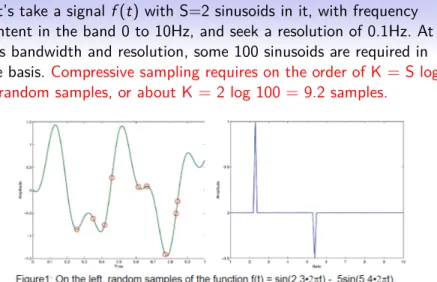
Let’s take a signal f (t) with S=2 sinusoids in it, with frequency content in the band 0 to 10Hz, and seek a resolution of 0.1Hz. At this bandwidth and resolution, some 100 sinusoids are required in the basis. Compressive sampling requires on the order of K = S log N random samples, or about K = 2 log 100 = 9.2 samples.

Figure : Signal sampling (time) and signal sparsity (frequency) by Lamoureux et al

(11)

Let’s take a signal f (t) with S=2 sinusoids in it, with frequency content in the band 0 to 10Hz, and seek a resolution of 0.1Hz. At this bandwidth and resolution, some 100 sinusoids are required in the basis. Compressive sampling requires on the order of K = S log N random samples, or about K = 2 log 100 = 9.2 samples.

Figure : L2 reconstruction (time) and Spectrum of the L2 reconstruction (frequency) by Lamoureux et al

IMAC2012 11/ 27

(12)

CS takes this idea one step further by creating a measurement system so that the real signal itself can be recorded in compressed form ”on the fly” = ⇒ A key step is the creation of measurement vectors φ for taking physical measurements on the signal in the form of inner products of the signal with the measurement vectors, y _k =< f , φ _k >. The measurement vectors are carefully designed to extract the maximum amount of information from a generically sparse vector in the given basis system.

Figure : Principe of CS

(13)

The optimization problem is replaced by a linearly constrained problem where the measurements of the signal must match the measurements on the representative solution. That is, one solves :

min

N

X

j=1

|a _j | st y _m =<

N

X

j=1

a _j ψ _j , φ _m >, m = 1...M (2)

IMAC2012 13/ 27

(14)

A simple, yet surprisingly effective, way to do so is L1 minimisation (or basis pursuit) ; thus

x ^∗ = argmin _x:φx=y kxk _l

1

(3)

results always compared to classical L2 norm x ^∗ = argmin _x:φx=y kxk _l

2

ou x ^∗ = (φ ^T φ) ⁻¹ φ ^T y pseudoinverse (4)

(15)

1D vibration example

Applications :

1

Long time monitoring (Bridge over a year)

2

Flutter diagnosis (Aircraft under operational loads) Limitations : No ”industrial” hardware

As an illustrative Matlab code ² ,let’s consider the case of a 1D signal (sparse in the frequency domain). We assume a function f (of length N) expressible in the form of a sum of a small number of sinusoids.

f = (1 ∗ sin(2pi ∗ 30 ∗ t ) + 0.5 ∗ sin(2pi ∗ 60 ∗ t) + 0.1 ∗ sin(2pi ∗ 100 ∗ t) + 0.1 ∗ sin(2pi ∗ 130 ∗ t))/4

2

L1-MAGIC is a collection of MATLAB routines : http ://users.ece.gatech.edu/ justin/l1magic/

IMAC2012 15/ 27

(16)

comparison of the reconstruction of signals

Analog signal (in BLUE Fs = 400Hz >> Nyquist frequency) has 4 frequency components 30, 60, 100 and 130 Hz

Regularly sampled at Fs = 150 Hz using L2 reconstruction formula (Shannon in MAGENTA)

L1 reconstruction (CS) with fewer points of observations (but random sample IN GREEN)

0 0.5 1 1.5 2 2.5

ï0.4 ï0.3 ï0.2 ï0.1 0 0.1 0.2 0.3 0.4

time (s)

Displacement

f = analog blue, f2 sampled magenta, b = random green

0 50 100 150 200

ï3 ï2 ï1 0 1 2 3 4

frequency (Hz) c = idct(f), idct(f2)

Spectrum Magnitude

Figure : Analog signal (in blue), discretized signal (magenta) respecting Nyquist frequency (N points) and randomized signals at low resolution (N/10) (a), and DCT spectrum comparison (b)

(17)

Sparse Basis and incoherent measurement system The sparse basis for this type of signal would be collections of sinusoids of the form sin(ωjt ), j=1...N, where the frequencies span the bandwidth at the desired resolution.

A suitable incoherent measurement system for this basis is to select random samples in the time domain, obtaining measurements yk = f(tk), where the tk, k=1...K, are selected randomly.

The L1 optimization problem is the constrained minimization (with 2N variables and K linear constraints) over the variables a _j ,

expressed in the form :

min

N

X

j=1

|a _j | st y m =

N

X

j=1

a j cos(ω j t m ), m = 1...M (5)

IMAC2012 17/ 27

(18)

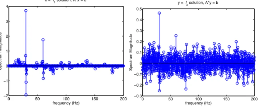
We see that the spectrum (DCT) has four resonances in the continuous signal, and 4 also in the digital signal but aliasing appears because Fs is too low. When we solve this problem using Moore- Penrose pseudoinverse, we can note the appearance of noise (whereas CS imposes zero coefficients).

0 50 100 150 200

ï2 ï1 0 1 2 3 4

x = l₁ solution, A*x = b

frequency (Hz)

Spectrum Magnitude

0 50 100 150 200

−0.3

−0.2

−0.1 0 0.1 0.2 0.3 0.4 0.5

frequency (Hz)

Spectrum Magnitude

y = l

2 solution, A*y = b

Figure : Comparison of DCT spectrum of reconstructed signals by L1 inversion (a) and L2 inversion (b) of randomized signals. The L2 inversion is not capable of good reconstruction (noise)

(19)

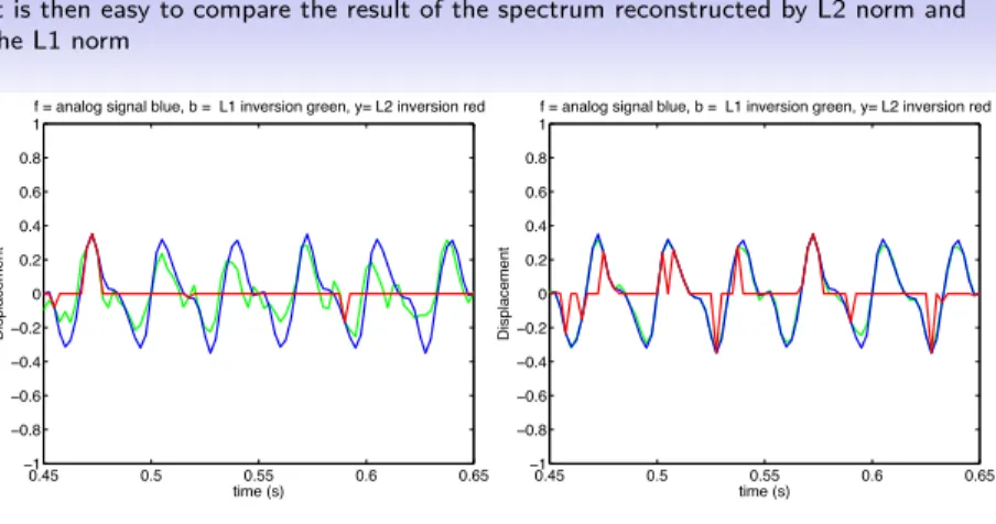
It is then easy to compare the result of the spectrum reconstructed by L2 norm and the L1 norm

0.45 0.5 0.55 0.6 0.65

ï1 ï0.8 ï0.6 ï0.4 ï0.2 0 0.2 0.4 0.6 0.8 1

time (s)

Displacement

f = analog signal blue, b = L1 inversion green, y= L2 inversion red

0.45 0.5 0.55 0.6 0.65

ï1 ï0.8 ï0.6 ï0.4 ï0.2 0 0.2 0.4 0.6 0.8 1

time (s)

Displacement

f = analog signal blue, b = L1 inversion green, y= L2 inversion red

Figure : Comparison of reconstructed signals by L1 inversion (green) for different sampling N/10 (a) and N/5 : (b) of randomized signals. From the time domain (zoom) The L2 inversion (red) is not capable of good reconstruction of the continuous signal (blue) whereas L1 optimization (green) is reliable even for low sampling.

IMAC2012 19/ 27

(20)

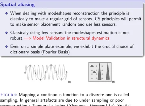
Spatial aliasing

When dealing with modeshapes reconstruction the principle is classicaly to make a regular grid of sensors. CS principles will permit to make sensor placement random and use less sensors.

Classicaly using few sensors the modeshapes estimation is not robust.= ⇒ Model Validation in structural dynamics

Even on a simple plate example, we exhibit the crucial choice of dictionary basis (Fourier Basis)

Figure : Mapping a continuous function to a discrete one is called sampling. In general artefacts are due to under sampling or poor reconstruction : Temporal aliasing (Shannon’s theorem) (a), Spatial aliasing (b) due to limited spatial resolution and induce loss of details.

(21)

As a first example we study the modeshape reconstruction from grid placement. It highlights the fact that mode shapes

visualization is often biased due to spatial aliasing. We can see that 9 grid point measurement are not enough precise to reconstruct the (2, 1) mode shape.

Figure : (2,1) mode of vibrating plate plus regular grid distribution of sensors in white circles (a) and The cubic interpolation which shows a spatial aliasing in mode shape reconstruction (b). A regular grid of 9 sensors permits only to reconstruct the (0,1).

IMAC2012 21/ 27

(22)

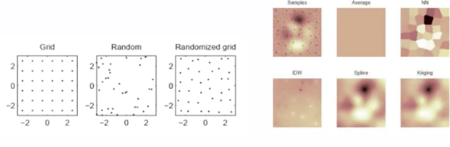
Experimentaly modeshapes are commonly estimated from the residues obtained by curve fitting algorithm from set of FRFs. This numerical study can be compared to experimental test where Laser Doppler Vibrometer can be moved automatically and so control the succession of acquisition for each point of the grid (regular or random).

What kind of Sampling ? What are the best reconstruction scheme ?

Figure : Previous IMAC (2009) we test 3 different sampling and interpolation methods have been tested and compared using simulated (peaks) data

(23)

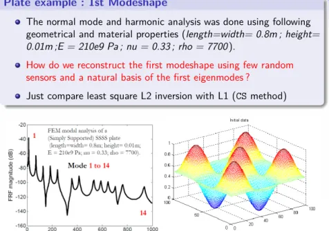
Plate example : 1st Modeshape

The normal mode and harmonic analysis was done using following geometrical and material properties (length=width= 0.8m ; height=

0.01m ;E = 210e9 Pa ; nu = 0.33 ; rho = 7700 ).

How do we reconstruct the first modeshape using few random sensors and a natural basis of the first eigenmodes ?

Just compare least square L2 inversion with L1 (CS method)

Figure : Vizualisation one FRF of the SSSS plate example and mode 14

(24)

Sparse Basis and incoherent measurement system The sparse basis for this type of signal would be collections of modeshapes (sin(ω j t m /a)) ∗ (sin(ω j t m /b)) at the desired resolution (5x5 modes).

A suitable incoherent measurement system for this basis is to select random samples (6 sensors) in the space domain, obtaining

measurements yk = f(tk), where the tk, k=1...K, are selected randomly.

(25)

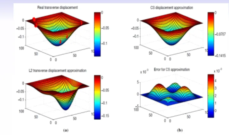
First Result L2 vs L1 reconstruction

Figure : First modeshape reconstruction. L2 vs L1 and error versus continuous modeshape (maximum error of 5E − 3)

= ⇒ Just a premilinary results, we need to analyse the RMSE for mode 1 to 14, and even on this simple example, automating the

procedure will be complex

IMAC2012 25/ 27

(26)

Second Result L2 vs L1 reconstruction (12 sensors, 14x14 modes)

Figure : Higher modeshape reconstruction. L2 vs L1 and error versus continuous modeshape (maximum error of 4E − 2)

(27)

Conclusion and Future works

These promising results induce lot of numerical works in order to establish adapted dictionnaries and automatic sensors placement tools for plate example (We only study the 1st Modeshape reconstruction).

We shall continue these works by merging different methods function of the modal density (Mixture of experts). For example, on should use L1 inversion at low frequency (dictonnary based on physical parameters) and interpolation such as neural networks for high frequency.

Use on complex structure : Assembly of plate/beam or thin walled structures...

The algorithm should also take into account the existence of nodal lines (passage to zero = a priori information)

IMAC2012 27/ 27

(28)

Joseph Morlier (ICA), Dimitri Bettebghor (ONERA)

Compressed sensing applied to modeshapes reconstruction:

Tutorial and (Very) First Results