Adaptive synthetic Schlieren imaging

(1)

Adaptive Synthetic Schlieren Imaging

by

Roderick R. La Foy

Submitted to the Department of Mechanical Engineering in Partial Fulfillment of the Requirements for the Degree of

Bachelor of Science at the

Massachusetts Institute of Technology June 2009 MASSACHUSETTS INSTITUTE OF TECHNOLOGY

SEP 16

2009

LIBRARIES

Adaptive Synthetic Schlieren Imaging

Roderick R. La Foy

Massachusetts Institute of Technology 1 Introduction

Schlieren photography has become an important tool in many fluid mechanical fields. The technique allows very small variations in the refractive index of a transparent fluid to be visualized meaning that other quantities that are important for analyzing the dynamics of the system, can be measured including density, pressure, temperature, and chemical concentration. Much of the fluid field information that is acquired using schlieren imaging, is very difficult or, in some circumstances, impossible to obtain with other methods.

Despite the utility of schlieren imaging, the technique is only commonly used in research institutions. This is due to both the large cost in designing a traditional schlieren system and to issues related to alignment, proper lighting, and other optical issues. Many of these problems can be addressed by using synthetic schlieren photography that uses apparent distortions in a high frequency background to infer the refractive index gradient field. Synthetic schlieren only requires using a traditional camera with a well-lit background, but the technique tends to produce low-resolution images. The resolution of these images can be significantly improved by using a technique herein described as adaptive synthetic schlieren imaging.

2 Synthetic Schlieren Imaging

Synthetic schlieren photography is relatively simple to implement and can be described using optical ray theory. When light passes through any medium in which the refractive index is not constant, refraction will cause the light rays to bend. By measuring these deflections, properties of the flow field can be inferred including changes in density and composition. Several optical techniques have been developed to image these refractive index gradients including shadowgraphy, interferometry, and traditional schlieren photography. Shadowgraphy involves imaging the changes in intensity produced in the shadows of light passing through a refractive index gradient while interferometry uses diffraction of a monochromatic light source to discern changes in the speed of light in different regions of a fluid due to the differences in the refractive index. Traditional schlieren photography is perhaps the most complex of these techniques. In traditional schlieren imaging, gradients in the refractive index normal to the imaging plane are viewed by focusing the deflected light rays onto a knife edge. The rays that are deflected above the knife edge appear as bright regions in the image while rays that are deflected onto the knife edge appear as dark regions in the image. By analyzing the image produced with traditional schlieren photography, the direction of the ray deflection can only be determined within a 1800 interval and thus only a limited knowledge of the refractive index field can be reconstructed. An improvement to this technique involves using a light source with multiple discrete colors placed in a known arrangement or using a light source with a continuous color gradient. Both of these techniques allow the angle of the ray deflections to be determined, but they add an additional level of complexity to the traditional schlieren system by requiring additional alignment and calibration.

(8)

In synthetic schlieren photography the gradient in the refractive index of the fluid is measured by comparing the apparent distortions in two or more images of a high frequency background. The fluid to be analyzed is placed between a camera and the background while the camera is focused at the background using a large depth of field. A diagram of a typical synthetic schlieren system is shown in Figure 1.

I

Figure 1: Schematic of a synthetic schlieren system including the camera, the refractive index gradient, and the high frequency background.

In this system, any local changes in the refractive index of the fluid result in regions of the high frequency background appearing to translate in the camera's image. To discern these translations, a reference image of the background is needed for comparison. The reference image is captured while the fluid is quiescent and the gradient in the refractive index is assumed to be identically zero. If the image intensity of the unperturbed field is represented by cI(x,y,O)

and the perturbed field image by cI(x,y,t) _{then magnitude of the gradient of the refractive index}

is given by

IVcN(x,y) = C - cI(x,y,0)-cI(x,y,t)[

where C is a constant that is a function of the geometry of the setup and the magnification of the camera lens.

While' theoretically any high frequency background can be used with synthetic schlieren, in practice two general backgrounds are predominantly used to minimize errors in the measurement. One background consists of a random and relatively dense pattern of dots. When this background is used, the reference image is compared by using an optical flow technique to measure the displacement of small interrogation windows within the camera image. The displacement vectors of these windows are proportional to the gradient in the refractive index. While using the random dot background directly gives the gradient field, the resolution of this technique is equal to the size of the interrogation windows that are typically at least 16 by

16 _{pixels. This effectively decreases the resolution of the camera image by a factor of 16. A}

second type of high frequency background is also used that has a significantly higher resolution, but in only one direction.

The second background commonly used in synthetic schlieren photography consists of a field of horizontal or vertical alternating black and white lines. The refractive index gradient is then found by subtracting the perturbed image from the reference image. In most regions, this will result in the intensity matrix being zero, but in any part of the image where there is a gradient in the refractive index normal to the direction of the lines, the intensity matrix will have a nonzero

(9)

value. Both of these methods are applied by either printing the background image on an opaque material and lighting it from the direction of the camera or by printing on a transparent material and using back lighting. An example of a typical random dot background and a typical lined background is shown in Figure 2.

3 Adaptive Synthetic Schlieren

While synthetic schlieren photography has several distinct advantages over traditional schlieren imaging, it has the distinct disadvantage of having a lower resolution. This lower resolution can be significantly increased by adaptively changing the high frequency background in real time while the data is collected.

Figure 2: a). A typical high frequency random dot background used in synthetic schlieren imaging. b). A typical

lined background used in synthetic schlieren.

This adaptive updating is accomplished by replacing the printed background or lit transparency background with a high-resolution LCD computer monitor and processing the images from the camera in real time. This process involves several distinct steps.

First, the camera must be calibrated to the LCD monitor. To correctly display the adaptively updated background, it is necessary to know the one-to-one transformation

slc(x,y) = T(clc(x,y)) between the monitor pixel coordinates and the camera pixel coordinates (where variables in camera coordinates are denoted by the left sub-script "C" and variables in screen coordinates are denoted by the left sub-script "S"). Further it must be possible to rapidly calculate the transformation of an image from camera coordinates to screen coordinates, thus this transformation must be computationally simple.

Once a suitable transformation is found, distortions in the refractive index can be found by subtracting the transformed camera image from the displayed screen image. The differenced image is then saved to the computers hard drive for analysis and further processing once the experiment is complete. The image resulting from the differencing operation tends to have high frequency noise due to the use of the high frequency background, thus to acquire a better approximation to the refractive index gradient, the differenced image is transformed with a low

(10)

pass filter. The low frequency image can then be used to calculate the new high frequency background.

The new background is calculated by scaling the low frequency signal to an appropriate range and based upon the local gradient in the image, using either the original horizontally lined image or an image that contains a black and white contour map of the refractive index gradient signal. The new background is then displayed on the monitor and a new iteration of the process is started.

4 Camera Calibration

In order for the adaptive process to function, it is crucial to know a one-to-one transformation between the camera coordinates and the screen coordinates. With this transformation, if a camera image centered on the computer monitor is given, it is possible to exactly reconstruct the image that is displayed on the monitor purely from camera data. Additionally, to maximize the refresh rate of the adaptive algorithm, it is necessary that this transformation can be rapidly calculated during each iteration. To facilitate this requirement, the transformation takes the form of an interpolation matrix that can be rapidly multiplied by the camera image matrix. This interpolation matrix is calculated by displaying a series of calibration images on the monitor while there are no perturbations in the fluid and comparing these known images to the output of the camera.

The region of the LCD monitor that displays the adaptive high frequency background has horizontal and vertical resolutions that are powers of two. This has two reasons: first, when a Fourier transform of the image is taken for filtering, the large reduction in calculation time by the fast Fourier transform can be utilized; and second, resolutions that are powers of two are the most convenient for the calibration technique that was developed.

The calibration technique involves displaying an image that is first vertically and then horizontally bisected into black and white pixels. Initially an image that is entirely black is displayed, then this image is continually bisected into black and white regions until sn

bisections are completed. The last iteration should display an image that alternates between black and white every other pixel. The ih iteration of an image to be displayed on the monitor that has a horizontal resolution of sN and a vertical resolution of sM is given by

sBx(x,y,i)= mod2[ X]

sB(x,y,i) = mod2 2m-]

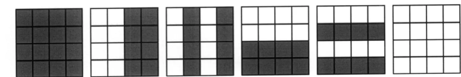
where i ranges from 0 to sn for sBx(x,y,i) and from 1 to sm for sB,(x,y,i) since i=O corresponds to an all black image in both functions. Figure 3 shows a series of calibration images for an image that has a resolution of 4 pixels by 4 pixels. An additional image that contains all white pixels is also included in the sequence for exposure compensation of the images and for the purpose of masking during the calibration calculation.

(11)

Figure 3: A series of bisected 4 pixel by 4 pixel images used calibrate the camera to the computer screen.

Once the sn+sm+2 calibration images have been acquired by the camera, cBx(x,y,i) and

cB,(x,y,i), the images are scaled such that the median value of the image with all black pixels equals zero and the median value of the image with all white pixels equals one. Any pixels that are less then zero after the scaling are set equal to zero and any pixels greater then one are set equal to one. This increases the reliability of the calibration method.

After the bisected images are scaled, the images are added together in a power series such that the summed image has an intensity that varies uniformly from 0 to sN-1 in the horizontal direction and from 0 to sM-1 in the vertical direction. Denoting these images as c Ix and c y

then

Sn

clIx(x,y) = cBx(x,y,i) -2'"

i-0

Sm

c I(x,y) = cB(x,y,i)2

sm-i-i=0

The rows and columns of the screen pixels in the camera coordinates are found by fitting polynomials to pixels in c x and cy whose intensity falls within a defined threshold r of variables j and k. To accomplish this, binary images are found from the thresholding arguments

Ic Ix(x,y)-jl< z

Iclv(x,y)- k[ <

where j is varied from 0 to sN- 1 and k is varied from 0 to sM-1. For each j and k, the non-zero pixels in the binary image are located and their coordinates are fit to an order P polynomial. The coefficients of the polynomial fit to the fh value inc l x are denoted by Px(j)

and the coefficients of the polynomials fitted to pixel coordinates in c y are given by P,(k). The polynomials model the distortion in the image due to the homography of the camera to the

LCD monitor and the lens distortion. Typically linear or quadratic polynomials were used, but wider-angle lenses or other factors might require higher order polynomials. Additionally, it may be possible to model the image distortion with other functions that take advantage of the fact that the lens distortion is likely radially symmetric and that the homographic distortion varies

linearly.

To find the camera coordinates (x*,y*) that correspond to the pixel (j,k) in the screen coordinates, the intersection of the polynomials x(j) and P,(k) are calculated using Newton's

MMEN MEMO

(12)

method to solve the system

= x- 1,y,y ,...,yY-']

0= y - [l,x ,...,x P -l ] .

for the coordinates x*(j,k) and y*(j,k) in the camera coordinate system. calculated for each j and k, an interpolation matrix that converts an coordinates to screen coordinates is created.

Once x* and y* are image from camera

Several different interpolation methods were considered, but an interpolation function that uses the eight nearest pixels and is quadratic in both x and y was selected due to its ease of calculation and symmetry about the pixel nearest to x* and y'. If the coordinates r and s are defined by

r = x*(j,k) - nint(x*(j,k)) s = y*(j,k) - nint(y (j,k))

1 1 1 1

where nint(x) is the nearest integer function, then -- < r <- and -- < s < - for all j and k.

2 2 2 2

Figure 4 shows a diagram of the relationship of (x*,y*) to the surrounding pixels in the (r,s)

coordinate system. The surrounding pixels are labeled from 1 to 9 corresponding to the nine interpolation coefficients h,(r(j,k),s(j,k)). r=- I r=O r= 4 .4 SI ' i . . . . . . . . .

i i

" I\ ! i .$, ,.. IP , ,,, . . .... ... +1 iI,... .... + !S _..._...

₊

= I'....4...

-Figure 4: A diagram of the (r,s) coordinate system used to interpolate the camera intensity values for transforming

from the camera coordinate system to the screen coordinate system.

The point (x*,y*) in the camera image corresponds to the center of the pixel at (j,k) in the screen coordinates. Thus in order to convert the camera image into screen coordinates, the jth

by kth pixel in the converted camera image should have the same intensity as the pixel located at (x*,y*), but since (x*,y*) is generally a non-integer pixel coordinate, cIc(x*,y*) has to be interpolated from the surrounding pixels. In this system the intensity is interpolated from the nine nearest pixels.

The interpolation is accomplished by defining the interpolated intensity as the sum of nine PY(k)

...

Y

t

(13)

coefficients multiplied by the corresponding pixel intensities. The following equation gives an interpolated intensity

9

slc(j,k)= h,(r(j,k),s(j,k))'cc(x,,y,)

i=1

corresponding to the screen coordinate (j,k) where (xi,y,) are the relative pixel coordinates as shown in Figure 4. The nine interpolation functions are given by

1 h, (r,s) - -(1 + r) -( + s) -r -s 4 1

h2(r,s

) - -

(1- )(1

r)-" + s) r" s 4 1 h3(r,s) = _-

)

( - - s) r s 4 1 h4(T,S) = -- (1+ r) (1- S) r s 4 1 h,6(r,s) = -- (1 - r) (1 + )- rs(1 - r) 2 1 h,(r,s) = - A - ( 1 - r) -(1l+ r). r s(- s) 2 1 2 h8(r,s) =- A (1 + s)'(1- s)" r (1 + r) h,(r,s) = (1 + s) -(1 - s) -(l + r) -(l - r)

To minimize the time required to complete the transformation of the camera image into screen coordinates, matrix multiplication is used. The matrix containing the camera image data is converted into a vector by concatenating the columns of the camera image together such that the camera vector cic is given by

c c(J)=clc( + mod m(j- 1), -M

where j is in the domain from I to cN-cM. This operation is generally easy to implement since most programming languages already store matrices as concatenated column vectors.

The interpolation matrix A is a cN-cM by cN-cM matrix and is therefore very large even for a relatively low-resolution camera image. Each row of A only has nine non-zero elements corresponding to the nine elements of the interpolation function h(r,s), thus the interpolation matrix may be represented as a sparse matrix in order to conserve computer memory. To calculate A, sN-sM rows are filled in with the appropriate nine interpolation functions for each

(14)

by

sic = A-cic

which can be converted back into matrix form using the function

slc(j,k)=sc(cM -(k -1) + j).

Then since slc(j,k) has the same resolution as the camera, cN by cM, only the first sN by

sM elements of the interpolated image matrix are taken for the differencing operation in synthetic schlieren.

5 Adaptive Background Modification

Once the transformation between the screen and camera coordinates is known, data can be collected. Initially, the gradient in the refractive index of the fluid is not known, therefore an arbitrary initial background image must be chosen for the first iteration. Since the gradient field can be calculated from the lined image relatively simply, this is chosen for the initial image. Then if the intensity matrix of the lined image is given by sIL(Sx,Sy) then an approximation to the gradient field given by

IVN(sx,s y) = C- I,(x, y) - T(c Ic (x, y))l = C. AI(x,y)

where clc(x,y) is the image captured from the camera and C is a constant of proportionality. This approximation has a large degree of noise due to the linear geometry of the response as is illustrated in Figure 5a which shows convection currents generated by a soldering iron. The noise in the subtracted image is then removed by applying a low pass filter to the image.

The low pass filter is applied by converting the image to frequency space and multiplying this result by a Gaussian function as given by

x2+y2

sAI(x,y)= F-'(F(sMA(x,y))-e 4 , )

where F(x,y) and F-'(x,y) correspond to the two dimensional Fourier transform and the inverse two dimensional Fourier transform respectively and ar controls the frequency of the signal that passes. Once the filtered image is obtained, it must be transformed to an image suitable for being displayed as the new high frequency background.

(15)

Figure 5: a). The image produced by subtracting the perturbed image from the horizontally lined reference image.

b). Image a processed with a low pass filter.

The error in the calculated refractive index gradient field is reduced by using high contrast background images. When synthetic schlieren systems are designed using a random dot background, higher contrast backgrounds result in higher amplitude correlation peaks when using a phase correlation technique to calculate optical flow. This results in the optical flow algorithm choosing fewer incorrect phase correlation peaks and therefore an overall smaller error in the calculated field. Higher contrast backgrounds decrease the error when using lined backgrounds as well.

When high frequency lined images are used for a background, the apparent translation of the lines is proportional to the component of gradient of the refractive index that is normal to the direction of the lines. If the lines are translated by a distance that is less then half of the period of the lines, then the difference between the camera image and the reference image will have a value that is a weighted average of the intensity of the light and dark lines. Since the camera has a limited dynamic range, the sensitivity of the camera to the weighted average will be

maximized by maximizing the difference between the intensity values of the light and dark lines. Therefore maximizing the contrast in the lined background image will maximize the sensitivity of the synthetic schlieren method.

When the lined background image is used, the strongest amplitude signal occurs when the gradient in the refractive index is normal to direction of the lines. This remains true regardless of the orientation of the lines, therefore the optimal image to display on the monitor is an image in which there are a series of high contrast lines that are everywhere normal to the refractive index gradient. This can be accomplished by scaling the lowpass filtered image so that all intensities lie within the interval between zero and one with the function

A, _max(sA,sMIL -min(sALP)₎

- min(s Ap)

Then to create a high contrast image that has lines everywhere normal to the gradient, the modulus base 2 is taken of the scaled image multiplied by a constant nL that equals the number black to white transitions that will be displayed. This transformation is given by

(16)

The black and white regions that are created using this transformation transition relatively rapidly in regions where the absolute value of the gradient is large, but in most regions, the resolution is in fact lower than when either the random dot image or lined image is used as a background. An example image produced using this method is shown in Figure 6 in which the sparse and dense regions are apparent.

Figure 6: a). An image produced by taking the modulus base two of the rescaled andfiltered difference image. The transformation used to create the background image can be modified to cause the entire image to be densely contoured. This is accomplished by calculating the gradient in SAILP and choosing the horizontally lined image when the gradient is below some threshold. In order to increase the speed of the calculation of the gradient, a Sobel filter defined by

(- 1 -2 - 1'

h=

0

-1 -2 -1/

and it's transpose are convoluted with sMLp. _{This method is faster than calculating the finite} difference matrix since the frequency space of sAI, is already known _{from the smoothing} operation. The total gradient approximation is then given by

IVsAIL,,

P

sAlP, * h +

lsAI,

* hT .

Then the adaptive image is given by

s Di=sMod

(IVSAILP

_{< rV)+SL -( VSAILP,} _I_< _V)C

where S Mod is the image produced by the modulus _{transformation} _and

s, is the image consisting of horizontal lines.

The iteration of the adaptive synthetic schlieren algorithm is then completed by saving the image Dis _{and displaying it}_{as the new high frequency}_background_{on the computer monitor.} The system can then continue by capturing the next camera image and repeating the procedure.

(17)

4 Results

Several different experiments were completed to test the adaptive synthetic schlieren system. The first series of tests involved measuring the noise in sM(x,y) and the quality of synthetic schlieren images created in the screen coordinate system, since typically synthetic schlieren images are calculated in the camera coordinate system. Once it was confirmed that high-resolution synthetic schlieren imaging could be completed in the screen coordinates, several experiments were conducted to measure the adaptive capabilities of the system.

The primary experiment involved imaging a jet of compressed gas exiting a nozzle. This experiment has the advantage that near the nozzle, the flow is approximately steady state and at larger distances, where the flow becomes turbulent, ensemble averaging could be completed to obtain a steady-state adaptively modified background that gives higher precision than using horizontal or vertical lines.

The noise in the signal sM(x,y) is primarily due to errors in the camera calibration and in the creation of the interpolation matrix A. The camera calibration errors result from distortion, blurring, and incorrect exposure in the bisection images cBx(x,y,i) and cBy(x,y,i); edge effects in the reconstructed imagescx and c I; and from approximating the screen image distortion in the camera images by polynomials. These errors result in the polynomial intersections (x*,y*) having small differences from the actual values. The errors in the interpolation matrix are then due to incorrectly calculating (x*,y*) and to incorrectly interpolating the intensity clc(x*,y*). Despite these possible sources of error, the noise in sM(x,y) is

relatively low compared to the signal strength.

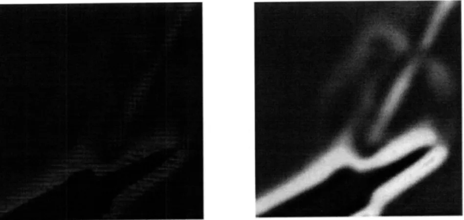
The noise strength was estimated by displaying a uniform image on the computer screen and then calculating sMA(x,y) from this image. Figure 7 shows an average of the noise from fifty image acquisitions. In this image the noise has been scaled to the full image quantization range to enhance visibility, but the noise lies between intensities of 12 and 23 while the signals produced from refractive index gradients lie between intensities 3 and 141.

Figure 7: The noise generated by the camera image coordinate transformation. With 256 quantization levels, the

(18)

In Figure 7, two predominant forms of noise are apparent. The first is the horizontal and vertical cross-hatching lines in the image and the second is the distorted checkerboard pattern. The horizontal and vertical lines are likely caused by errors in the fitting the of the polynomials to cIx

and c y _{since an offset in the position of the polynomials would cause some portions of an} image to receive lower intensities while adjacent to these regions a higher intensity would be apparent; several of the lines appear to come in pairs of lighter and darker regions adjacent to one another which supports this theory. The checkerboard pattern may be caused by pixel aliasing in the interpolation matrix, but this is unknown.

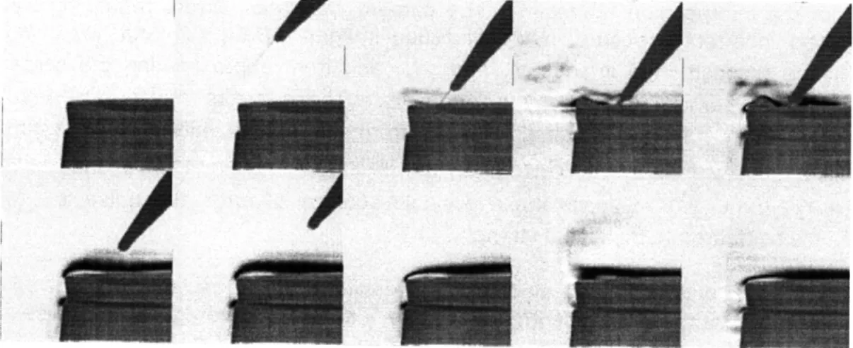
As a first experiment to ensure the validity of synthetic schlieren in the screen coordinate system, a chemical vapor mixing with air was visualized. In the experiment, a cylinder was placed in the field of view of the camera in front of the computer monitor displaying a high frequency horizontally lined background and a small amount of acetone was poured on the end of the cylinder. Figure 8 shows a time series of the experiment in which evaporating acetone

mixing with the surrounding air is apparent.

Figure 8: A time series using synthetic schlieren imaging in the screen coordinate system to show acetone

evaporating and mixing with air

Once it was established that high-resolution synthetic schlieren images could be produced in the screen coordinate system, the high frequency background was adaptively updated. For these experiments, a steady-state jet flow from a compressed gas flowing through a nozzle was used. Initially, the horizontally lined high-frequency background was used to estimate the refractive index gradient. Once sAI(x,y) _{was calculated using the lined background, the}

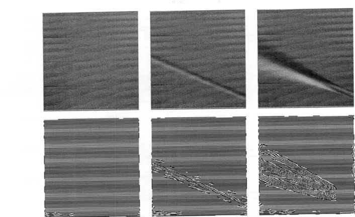
background was modified using the procedure described in section 5. Figure 9 shows a time series of the compressed gas jet with sAI(x,y) _{shown in the top three images and} _siP_{in the}

(19)

Figure 9: Top row: a series of unfiltered synthetic schlieren images of a steady-state jet flow; bottom row: a series

of adaptively updated high frequency backgrounds that were calculated from the top images.

In these images, some errors are apparent in the series of sIDisp on the perimeter of the images. These errors are partially due to the edge effects in calculating the interpolation matrix A, but they are primarily caused by the low pass filtering operation. The low pass filter was applied in Fourier space that has a false high-frequency signal due to the abrupt edges in the image. This effect is mostly eliminated by using the discrete cosine transformation (DCT) instead of the discrete Fourier transformation since the DCT is less subject to these boundary effects.

5 Conclusions

Synthetic schlieren photography offers many advantages over traditional schlieren techniques, but tends to be limited by an inherently lower resolution due to the constraints of a static background. Adaptive synthetic schlieren imaging increases this resolution by continually changing the background in a manner that maximizes the response of the computational image to spatial changes in the refractive index. This allows a schlieren imaging system to be designed that has a resolution that is only limited by the capabilities of the camera and monitors used, while remaining relatively low cost.

The primary limitations with the adaptive synthetic schlieren system described here are based in hardware. The resolution of the system could be increased by using both a higher resolution monitor and a higher camera. A camera with more quantization levels as well as a higher contrast monitor could also improve the method. Additionally since the utility of the method is inherently based upon the ability to refresh the background image displayed on the monitor at a high rate, using a computer with a large processing power and a fast hard drive can also result in significantly improved results.

(20)

synthetic schlieren techniques, but offers a significant advantage in resolution. This higher resolution potentially will allow flows that could only be visualized with traditional schlieren before, to now be visualized using adaptive synthetic schlieren.

References

SUTHERLAND, B., DALZIEL, S., HUGHES, G., and LINDEN, P. 1999. Visualization and Measurement of Internal Waves by "Synthetic Schlieren". Part 1: Vertically Oscillating Cylinder.

Journal of Fluid Mechanics 390, 5-12.

GREENBERG, P., KLIMEK, R., and BUCHELE, D. 1995. Quantitative Rainbow Schlieren Deflectometry. Applied Optics 34, 3811-3813.

PAN, C. 2001. Gibbs Phenomena Removal and Digital Filtering Directly through the Fast Fourier Transform. IEEE Transactions on Signal Processing 49, 444-445.

GONZALEZ, C., and WOODS, R. 2002. Digital Image Processing. Prentice-Hall, Inc. 2nd Ed.

BURDEN, R. and FAIRES, J. 2005. Numerical Analysis. Thomson Brooks/Cole. 8th Ed. BATHE, K. 2006. Finite Element Procedures. Prentice Hall, Pearson Education, Inc. 1st Ed.

(21)

APPENDIX A MATLAB Code

These are the MATLAB functions that were used to complete the adaptive synthetic schlieren project.

function calibrate test v02;

% This defines the screen resolution scr xres=256;

scr_yres=256;

% If this variable is set to zero, MATLAB will load a calibration file from the harddrive; if it is set % equal to 1i, the code will go through the calibration process calibrate=0; if calibrate==l; [I_X,I_Y,I_Cam]=monitor_calibrate_images(scr_xres,scr_yres); cam xres=size(I_Cam,2); cam_yres=size(I_Cam,1); M_Interp=screen_calibrate_v04(I_Cam,I_X,I_Y,scr_xres,scr_yres); save('M_Interp.mat','M_Interp'); else; load('M_Interp.mat'); end;

% This gets the monitor resolution v=get(0,'ScreenSize');

mon_xres=v(3); mon yres=v(4);

% This creates a directory to save data in directory=[pwd,'\Test01\'];

mkdir(directory);

% This defines the low pass filter; a Gaussian function is multiplied by the frequency space component and mask_rad is the standard deviation of the Gaussian function

maskrad=5;

M=lp_filt(mask_rad);

% This creates a Sobel filter for calculating the gradient h_filt=fspecial('sobel');

% This defines the number of transitions in the modulus image n trans=80;

% This calibrates the exposure by taking images of a mostly black screen % and a mostly white screen

I_B=zeros(scr_yres,scrxres); I W=ones(scr_yres,scr_xres); IB Monitor=padarray(I_B,[(mon_yres-scr yres)/2,(monxres-scrxres)/2],'both'); I W Monitor=padarray(I_W,[(mon_yres-scr_yres)/2,(monxres-scr_xres)/2],'both'); vid_object=cam_init(350,7.5,430); fullscreen(I_BMonitor,l); pause(l); I_Cam=double(cam_imag aq(vid_object)); IMin=median(I_Cam(:));

(22)

fullscreen(I WMonitor,l); pause(l);

I Cam=double(cam_imagaq(vidobject));

IMax=median(ICam(:));

% This creates the original horizontally lined image to be displayed as the background n=1; [X,Y]=meshgrid(l:scr_xres,l:scr_yres); I=mod(floor((Y-1)/n),2); I_Monitor=padarray(I,[(monyres-size(I,1))/2,(monxres-size(I,2))/2],'both'); fullscreen(I Monitor,l);

% This is the number of frames to smooth data over; this decreases errors due to turbulence

winnum=1;

I Filt Hist=zeros(scr_yres,scr_xres,win_num); for n=1:50;

% This grabs a frame from the camera

I_Cam=double(cam_imag_aq(vid_object)); cam xres=size(I_Cam,2);

cam_yres=size(I Cam, 1);

% The camera frame is multiplied by the interpolation matrix IReconLin=M_Interp*I_Cam(:);

I_Recon=reshape(I Recon_Lin,cam yres,cam_xres);

% The image is scales so that white pixels on the screen roughly correspond to an intensity of one and % % black pixels correspond to an intensity of zero

I_Recon_Crop=I_Recon(l:scryres,l:scr_xres); I_Recon_Crop=(I_Recon_Crop-I_Min)/(I_Max-IMin); % This calculates the difference image

I Diff=abs(I Recon_Crop'-I); % And applies a low pass filter

Y=fftshift(fft2(I_Diff)); Y Filt=Y.*M;

I_Filt=real(ifft2(ifftshift(Y_Filt))); % This averages win_num frames together

if n>win num; IFilt_Hist(:,:,1l)=[]; I_Filt_Hist(::,,win_num)=I_Filt; I_Filt Avg=sum(I_Filt_Hist,3)/win_num; else; I_Filt_Hist(:,:,n)=I_Filt; I_Filt_Avg=sum(IFilt_Hist,3)/n; end; I_Filt=I Filt_Avg;

% This creates the modulus image

I Mod=mod(round(I_Filt*n_trans),2);

% This calculates the image gradient DY I Filt=imfilter(I_Filt,h_filt); DX I Filt=imfilter(IFilt,h_filt');

DI Filt=image_norm(abs(DX_I_Filt)+abs(DYIFilt)).^(0.5); D I Filt=D I Filt>0.13;

% This creates the image to be displayed next on the monitor I_Disp=DI_Filt.*I Mod+(l-D_IFilt).*I;

% This saves the image displayed as well as the signal image I_Save_l1=uint8(255*IDisp);

I Save_2=uint8(round(255*(I_Diff))); filename_l1=['imgl_ ',num2str(n),'.tif']; filename_2=['img_2_ ',num2str(n),'.tif'];

imwrite(I _Save_1,[directory,filename_ 1],'tif');

imwrite(I Save_2,[directory,filename_2],'tif'); % This displays the new background image

(23)

I_Monitor=padarray(I_Disp,[(mon_yres-scr yres)/2,(monxres-scr_xres)/2],'both');

fullscreen(I_Monitor,1); I=I_Disp;

% This displays the signal image on the other monitor if n==l; figure(2); h=imagesc(I_Diff,'EraseMode','none',[0,1]); colorbar; colormap('gray'); truesize; %imshow(I_Out); title(n); else; figure(2); set(h,'CData',I_Diff); %imshow(I_Out); title(n); end; pause(0.01); end; pause(2); closescreen; cam_close(vid_object); function M=lp_filt(sigma); % This is a low pass filter xres=256; yres=256; %sigma=30; [X,Y]=meshgrid(l:xres,l:yres); X=X-xres/2; Y=Y-yres/2; M=exp(-(X/(2*sigma)).^2-(Y/(2*sigma)).^2); function I_Out=image_norm(I_In);

% This scales an image to lie between zero and one I_Out=(I_In-min(I_In(:)))/(max(I_In(:))-min(I_In(:)));

function [I_X,I_Y,I_Cam]=monitor_calibrate_images(scrxres,scr_yres);

% This displays the bisected calibration images and creates the IX and I Y

matricies

% This is the resolution to be displayed on the LCD monitor %scrxres=512;

%scryres=512;

% This is the screen resolution v=get(0,'ScreenSize');

mon_xres=v(3); mon_yres=v(4);

% This defines the image matrix

M=zeros(scryres,scr_xres,log2(scr_xres)+log2(scryres)+2); % This defines the binary decompositions of the screen ypow=log2(scr_yres)+1;

(24)

xpow=(log2(scr_xres)-n)+l; M(:,:,n)=screen_bisect(scr_xres,scr_yres,xpow,ypow); end; xpow=log2(scrxres)+1; for n=l:log2(scr_yres)+l; ypow=(log2(scr_yres)-n)+l; M(:,:,n+log2(scrxres)+l)=screenbisect(scr_xres,scr_yres,xpow,ypow); end; M(:,:,end+l)=ones(scr yres,scrxres); M_Pad=zeros(mon_yres,mon_xres,size(M,3)); %vid_object=caminit(350,7.5,430); vid_object=caminit(500,7.5,900); for n=l:size(M,3); M_Pad(:,:,n)=padarray(M(:,:,n),[(mon_yres-scr_yres)/2,(mon_xres-scr_xres)/2],'both'); if (size(M_Pad,l)-=mon_yres)l l(size(M_Pad,2)-=mon_xres); break; else; fullscreen(M_Pad(:,:,n),l); pause(2); ICam(:,:,n)=camimag_aq(vid_object); pause(l); if n==size(M,3); closescreen; end; end; end; cam_close(vid_object); v_low=double(median(median(I_Cam(:,:,1)))); v_high=double(median(median(I_Cam(:,:,end)))); I_Cam=double(I_Cam); I_Cam=255*(I Cam-v_low)/(vhigh-v_low); I_Cam=O*(I_Cam<O)+I _Cam.*(I_Cam>=O); I_Cam=255*(I_Cam>255)+ICam.*(I_Cam<=255); I_Cam=uint8(round(I_Cam)); I_Cam=image_norm(double(I Cam)); cam_xres=size(I_Cam,2); cam_yres=size(ICam,1); I_X=zeros(cam_yres,cam_xres); I_Y=zeros(cam_yres,cam_xres); for n=l:(size(M,3)-1)/2; I_X=I_X+(I_Cam(:,:,n)>0.5)*2^((size(M,3)-l)/2-n); I_Y=I_Y+(I_Cam(:,:,n+(size(M,3)-1)/2)>0.5)*2^((size(M,3)-l)/2-n); end;

% The median filter is to eliminate noise due to pixel aliasing. A better % operation would be to find any locations of I_X and I_Y that have a large % gradient in intensity and apply the median filter there.

I_X=medfilt2(I_X,[3,3]); I Y=medfilt2(I_Y,[3,3]); % imagesc(I_X); % axis equal; % colormap('hsv'); % pause; function I=screen_bisect(scr_xres,scr_yres,xpow,ypow); % This creates bisected screen images

[X,Y]=meshgrid(l:scr_xres,l:scr_yres);

(25)

function vid_object=cam init(gain,framerate,shutter); % This initializes the camera

% This is a list of possible video formats with the Flea 2 % 1: 'F7 Y16 1288x482' Framerate: Default

% 2: 'F7 Y16 1288x964' Framerate: Default

% 5: 'F7 Y8 1288x482' Framerate: Default % 6: 'F7 Y8 1288x964' Framerate: Default % 7: 'F7 Y8 644x482' Framerate: Default % 8: 'F7 Y8 644x964' Framerate: Default % 9: 'Y16_1024x768' Framerate: {3.75,1.75} % 10: 'Y16_1280x960' Framerate: {1.75} % 11: 'Y16_640x480' Framerate: {7.5,3.75} % 12: 'Y16_800x600' Framerate: {7.5,3.75} % 13: 'Y8_1024x768' Framerate: {7.5,3.75,1.75} % 14: 'Y8_1280x960' Framerate: {3.75,1.75} % 15: 'Y8_640x480' Framerate: {15,7.5,3.75,1.75} % 16: 'Y8_800x600' Framerate: {15,7.5} vid format=13; % Y8 1024x768 dcam_info=imaqhwinfo('dcam'); if isempty(cell2mat(dcam_info.DeviceIDs)); error('DCAM device not found.');

else;

% This acquires device information dcam_info=imaqhwinfo('dcam',l1);

% This creates the video object with the specified format

vidobject=videoinput('dcam',l,char(dcaminfo.SupportedFormats(vidformat))); % This sets the number of frames per trigger to 1

set(vid_object,'FramesPerTrigger',l1);

% This sets the number of triggers to infinity set(vid_object,'TriggerRepeat',Inf);

% This sets the type of trigger triggerconfig(vid_object,'manual'); % This sets the gain

set(getselectedsource(vid_object),'Gain',gain); % This sets the framerate

set(getselectedsource(vid_object),'FrameRate',num2str(framerate)); % This sets the shutter

set(getselectedsource(vid_object),'Shutter',shutter); disp(get(getselectedsource(vidobject)));

% This initializes the camera start(vid_object);

% And checks that the camera did initialize if isrunning(vid_object)==0;

error('Cannot initialize Flea 2.'); end;

end;

function I=cam_imag_aq(vid_object); % This acquires camera images

% This verifies that the camera is still initialized if isrunning(vidobject)==0;

error('Flea 2 is not initialized.'); else;

(26)

% This triggers the camera to aquire a frame trigger(vid_object);

% This waits for the camera to aquire the frame while islogging(vid_object)==1;

pause(0.001); end;

% This saves the frame to the matrix I cam data=getdata(vid_object,l);

I=cam_data(:,:,1,1); end;

function cam close(vid_object);

% This stops the camera from acquiring images and deletes the video object stop(vid_object);

delete(vidobject); clear('vid_object');

function [XO,YO]=more diff func intersect;

% This finds the intersection of the fit polynomials global X_Poly_Fit;

global YPolyFit; global cam xres; global cam_yres; global scrxres; global scr_yres;

tol=(le-2)^4;

xi=cam xres/2-scr xres/2:cam xres/2+scr xres/2-1; yi=cam_yres/2-scr_yres/2:cam_yres/2+scr_yres/2-1; [Xi,Yi]=meshgrid(xi,yi); dSi=ones(size(Xi)); while max(dSi(:))>tol; Fl=Yi-polyval_matrix_X(Y_Poly_Fit,Xi-cam_xres/2); F2=Xi-polyval_matrix_Y(X_Poly_Fit,Yi-camyres/2); J11=-polyval_matrix_X(polyder_matrix(Y_Poly_Fit),Xi-cam_xres/2); J12=ones(size(Xi)); J21=ones(size(Xi)); J22=-polyval_matrix_Y(polyder_matrix(X_Poly_Fit),Yi-camyres/2); dXi=(F2.*J12-Fl.*J22)./(Jil.*J22-J21.*J12); dYi=(F1.*J21-F2.*J11)./(JIl.*J22-J21.*JI2); Xi=Xi+0.5*dXi; Yi=Yi+0.5*dYi; dSi=realpow(dXi,2)+realpow(dYi,2); pause(0.001); end; XO=xi; YO=Yi; function Y=polyval_matrix_X(P,X); Y=zeros(size(X)); for j=l:size(X,2); Y(:,j)=polyval(P(j,:),X(:,j)); end;

(27)

function X=polyval_matrix_Y(P,Y); X=zeros(size(Y)); for k=l:size(Y,1); X(k,:)=polyval(P(k,:),Y(k,:)); end; function dP=polyder_matrix(P); P=P(:,l:end-l); [Pwr_Vect,P_Length]=meshgrid(fliplr(l:size(P,2)),1:size(P,1)); dP=P.*PwrVect; function [X_Poly_Fit,Y_Poly_Fit]=image-polyfit(IX,I-Y,scr-xres,scryres,camxrescamyres,p olyorder,thresh); X_Poly_Fit=zeros(scr_xres,poly_order+l); Y_Poly_Fit=zeros(scr_yres,polyorder+1); for j=l:scr_xres; I_Line=abs(I_X-j)<thresh; ILine Ones=find(I_Line); if length(I_Line_Ones)>poly_order;

[ones_yindx,ones xindx]=ind2sub(size(I Line),I LineOnes); P=polyfit(ones_yindx-cam_yres/2,ones_xindx,poly_order); X_Poly_Fit(j,:)=P; else; X_Poly_Fit(j,:)=zeros(l,poly_order+l); end; pause(0.001); end; for k=l:scr_yres; I_Line=abs(I_Y-k)<thresh; I_Line_Ones=find(I_Line); if length(I_Line_Ones)>poly_order; [ones_yindx,onesxindx]=ind2sub(size(ILine),ILineOnes); P=polyfit(ones_xindx-cam_xres/2,ones_yindx,poly_order); Y_Poly_Fit(k,:)=P; else; X_Poly_Fit(k,:)=zeros(l,poly_order+l); end; pause(0.001); end; function M_Interp=interp_matrix_one(px,py,camxres,cam_yres); global X_Poly_Fit; global YPoly_Fit; px=px.*(round(px)-=0)+2*(round(px)==0); py=py.*(round(px)-=0)+2*(round(py)==0); x_near=round(px); y_near=round(py); r=px-x near; s=py-y_near; h=nine_node_interp(r,s); [J,K]=meshgrid(l:size(px,l),l:size(px,2));

(28)

lin indx_jk=sub2ind([cam_yres,cam_xres],J,K); linindx_h=zeros(size(px,l),size(px,2),9);

linindx_h(:,:,l)=sub2ind([cam_yres,cam xres],y_near+1,x_near+l); linindx_h(:,:,2)=sub2ind([cam yres,camxres],y_near+l,x_near-1); lin indx_h(:,:,3)=sub2ind([cam_yres,cam_xres],y_near-l,x_near-1); lin indx_h(:,:,4)=sub2ind([cam_yres,cam xres],y_near-l,x_near+l); lin indx_h(::,:,5)=sub2ind([cam yres,cam_xres],y_near+l,x_near+); lin indx_h(:,:,6)=sub2ind([camyres,cam xres],y_near+O,x_near-1); lin indx_h(:,:,7)=sub2ind([cam_yres,camxres],y_near-l,x_near+O); lin indx_h(:,:,8)=sub2ind([cam_yres,camxres],y_near+O,x_near+l); lin indx_h(:,:,9)=sub2ind([camyres,camxres],ynear+O,x_near+O); m=O; J_Interp=zeros(size(px,l)*size(px,2)*9,1); K_Interp=zeros(size(px,l)*size(px,2)*9,1); V_Interp=zeros(size(px,l)*size(px,2)*9,1); for j=l:size(px,l); for k=l:size(px,2); for n=1:9; m=m+l; J_Interp(m)=lin_indx_jk(j,k); K_Interp(m)=lin_indx_h(k,j,n); if (sum(abs(X_Poly_Fit(j,:)))==0) I(sum(abs(Y_Poly_Fit(k,:)))==O); V_Interp(m)=0; else; V_Interp(m)=h(k,j,n); end; end; end; end; M_Interp=sparse(J_Interp,KInterp,VInterpcamxres*camyres,camxres*camyres); function h=nine_node_interp(r,s); h=zeros(size(r,1),size(r,2),9); h(:,:,l) = (1/4)*(l+r).*(l+s).*r.*s; h(:,:,2) = -(1/4)*(1-r).*(l+s).*r.*s; h(:,:,3) = (1/4)*(1-r).*(1-s).*r.*s; h(:,:,4) = -(1/4)*(l+r).*(1-s).*r.*s; h(:,:,5) = (1/2)*(l-r).*(l+r).*s.*(l+s); h(:,:,6) = -(1/2)*(1-s).*(l+s).*r.*(l-r); h(:,:,7) = -(1/2)*(1-r).*(l+r).*s.*(l-s); h(:,:,8) = (1/2)*(l+s).*(1-s).*r.*(l+r); h(:,:,9) = (1+s).*(l-s).*(1+r).*(l-r);

function M_Interp=screen calibrate_v04(I_Cam,I_X,I_Y,scrxres,scr_yres); global X_Poly_Fit;

global Y_Poly_Fit; global cam xres; global cam_yres; global scr_xres; global scr_yres;

cam_xres=size(I_Cam,2); cam_yres=size(I_Cam,1);

% This section creates a mask that removes the outer pixels of the screen % image in order to reduce edge effects

(29)

I_Mask=imerode(I_Cam(:,:,end)>O,se); I X Mask=I X.*I Mask;

I Y Mask=I Y.*IMask;

% This fits polynomials of order poly_order to the gradients of I_X and I_Y % within a threshhold of thresh

thresh=1.5; poly_order=l;

[X_Poly_Fit,Y_Poly_Fit]=image_polyfit(I_X Mask,IY_Mask,scrxres,scr_yres,camxres, cam_yres,poly_order,thresh);

% This function finds the intersection points of the polynomials X_Poly_Fit % and Y_Poly_Fit

[XO,YO]=more_diff_func_intersect;

% The polynomials returned by image_polyfit have all zero coeeficients if % ill defined; the section below replaces the intersection points of any of % these polynomials with the nearest non-zero coeefficient intersection

[XPolyM-Mesh,YPoly Mesh]=meshgrid(sum(abs(X Poly Fit),2),sum(abs(YPolyFit),2)); Poly_Zeros=X_Poly_Mesh.*Y_Poly_Mesh; [y_poly_zeros,xpolyzeros]=find(Poly_Zeros==O); [X,Y]=meshgrid(l:scr_xres,l:scryres); Zero_Points=ones(scr_yres,scr_xres); for n=l:length(xpoly_zeros); Zero_Points(y_poly_zeros(n),x_polyzeros(n))=Inf; end; X=X.*Zero Points; Y=Y.*Zero Points; for n=l:length(x_poly_zeros); Dist_Sqr=abs(xpoly_zeros(n)-X)+abs(ypolyzeros(n)-Y); [min dist val,min x indx]=min(min(Dist_Sqr,[],1));

[min _dist_val,min y_indx]=min(min(Dist_Sqr,[],2));

XO(ypolyzeros(n),x_poly_zeros(n))=XO(min_y_indx,min x indx); YO(y_poly_zeros(n),x_poly_zeros(n))=YO(min_yindx,min x indx); end; px=XO; py=YO; M_Interp=interp_matrix_one(px,py,cam xres,cam_yres); function fullscreen(image,device_number)

%FULLSCREEN Display fullscreen true colour images

% FULLSCREEN(C,N) displays matlab image matrix C on display number N

% (which ranges from 1 to number of screens). Image matrix C must be

% the exact resolution of the output screen since no scaling in

% implemented. If fullscreen is activated on the same display

% as the MATLAB window, use ALT-TAB to switch back.

% If FULLSCREEN(C,N) is called the second time, the screen will update

% with the new image.

% Use CLOSESCREEN() to exit fullscreen.

% Requires Matlab 7.x (uses Java Virtual Machine), and has been tested on

% Linux and Windows platforms.

% Written by Pithawat Vachiramon

% Update (23/3/09):

% - Uses temporary bitmap file to speed up drawing process.

% - Implemeted a fix by Alejandro Camara Iglesias to solve issue with

(30)

ge = java.awt.GraphicsEnvironment.getLocalGraphicsEnvironment();

gds = ge.getScreenDevices();

height = gds(device_number).getDisplayMode().getHeight();

width = gds(device_number).getDisplayMode().getWidth();

if -isequal(size(image,l),height)

error(['Image must have verticle resolution of ' num2str(height)]); elseif -isequal(size(image,2),width)

error(['Image must have horizontal resolution of ' num2str(width)]); end

try

imwrite(image,[tempdir 'display.bmp']); catch

error('Image must be compatible with imwrite()'); end

buffimage = javax.imageio.ImageIO.read(java.io.File([tempdir 'display.bmp']));

global frame java;

global icon_java;

global device_number_java;

if -isequal(device_number_java, device number) try frame java.dispose(); end

frame_java = [];

device_number_java = device_number; end

if -isequal(class(frame_java), 'javax.swing.JFrame')

frame_java = javax.swing.JFrame(gds(device number).getDefaultConfiguration()); bounds = frame java.getBounds();

frame_java.setUndecorated(true);

icon_java = javax.swing.ImageIcon(buff_image); label = javax.swing.JLabel(icon_java);

frame_java.getContentPane.add(label);

gds(device number).setFullScreenWindow(frame_java); framejava.setLocation( bounds.x, bounds.y );

else iconjava.setImage(buffimage); end frame_java.pack frame_java.repaint frame_java.show function closescreen()

%CLOSESCREEN Dispose FULLSCREEN() window

global frame_java

Adaptive synthetic Schlieren imaging

SEP 16

2009

LIBRARIES

ARCHIVES

Adaptive Synthetic Schlieren Imaging

I

I

Ic Ix(x,y)-jl< z

i i

+

...

t

h2(r,s

(1- )(1

)

h=

0

0

0

P

lsAI,

(IVSAILP

₊