HAL Id: hal-00930991
https://hal.archives-ouvertes.fr/hal-00930991
Submitted on 21 Aug 2020
HAL is a multi-disciplinary open access
archive for the deposit and dissemination of sci-entific research documents, whether they are pub-lished or not. The documents may come from teaching and research institutions in France or abroad, or from public or private research centers.
L’archive ouverte pluridisciplinaire HAL, est destinée au dépôt et à la diffusion de documents scientifiques de niveau recherche, publiés ou non, émanant des établissements d’enseignement et de recherche français ou étrangers, des laboratoires publics ou privés.
Parameters of seismic source as deduced from 1 Hz
ionospheric GPS data: Case study of the 2011
Tohoku-oki event,
E. Astafyeva, L. Rolland, Ph. Lognonné, K. Khelfi, T. Yahagi
To cite this version:
E. Astafyeva, L. Rolland, Ph. Lognonné, K. Khelfi, T. Yahagi. Parameters of seismic source as deduced from 1 Hz ionospheric GPS data: Case study of the 2011 Tohoku-oki event,. Journal of Geophysical Research Space Physics, American Geophysical Union/Wiley, 2013, 118 (9), pp.5942-5950. �10.1002/jgra.50556�. �hal-00930991�
Parameters of seismic source as deduced from 1 Hz ionospheric
GPS data: Case study of the 2011 Tohoku-oki event
E. Astafyeva,1L. Rolland,2P. Lognonné,1K. Khelfi,1and T. Yahagi3
Received 29 April 2013; revised 1 July 2013; accepted 6 September 2013; published 19 September 2013.
[1] Following thefirst-time ionospheric imaging of a seismic fault, here we perform a case
study on retrieval of parameters of the extended seismic source ruptured during the great M9.0 Tohoku-oki earthquake. Using 1 Hz ionospheric GPS data from the Japanese network of GPS receivers (GEONET) and several GPS satellites, we analyze spatiotemporal characteristics of coseismic ionospheric perturbations and we obtain information on the dimensions and location of the sea surface uplift (seismic source). We further assess the criterion for the successful determination of seismic parameters from the ionosphere: the detection is possible when the line of sights from satellites to receivers cross the ionosphere above the seismic fault region. Besides, we demonstrate that the multisegment structure of the seismic fault of the Tohoku-oki earthquake can be seen in high-rate ionospheric GPS data. Overall, our results show that, under certain conditions, ionospheric GPS-derived TEC measurements could complement the currently working systems, or independent
ionospherically based system might be developed in the future.
Citation: Astafyeva, E., L. Rolland, P. Lognonne´, K. Khelfi, and T. Yahagi (2013), Parameters of seismic source as deduced from 1 Hz ionospheric GPS data: Case study of the 2011 Tohoku-oki event,J. Geophys. Res. Space Physics, 118, 5942–5950, doi:10.1002/jgra.50556.
1. Introduction
[2] A magnitude 9.0 earthquake struck off the eastern coast
of Japan at 05:46:23 UT on 11 March 2011. The quake oc-curred as a result of thrust faulting on or near the subduction zone interface plate boundary between the Pacific and North American plates. According to the US Geological Survey (The National Earthquake Information Center; http://earth-quake.usgs.gov), the hypocenter of this shallow earthquake is estimated at 32 km depth and located at 38.322°N and 142.369°E (Figure 1). Three minutes in duration, the earth-quake generated a tsunami on the Pacific coast from the Hokkaido, Tohoku, and Kanto regions, with tsunami maxi-mum heights of 38 m near the Ofunato region of Japan.
[3] Modeling of the rupture of this earthquake indicated that
the fault moved upward of 30–40 m and slipped over an area approximately 400 km long (along-strike) by 150 km wide (in the downdip direction). The rupture zone is roughly cen-tered on the earthquake epicenter along-strike, while peak slips were updip of the hypocenter, toward the Japan Trench axis
(http://earthquake.usgs.gov, Figure 1 and Figure 5). The rupture was bilateral, i.e., it spread away from the epicenter in both the north and south directions, taking about 2 min to cover a total of 400 km [e.g., Hayes, 2011; Simons et al., 2011].
[4] Such displacements of the ground and sea surface
caused strong ionospheric signals in the near-field of the earthquake’s epicenter [e.g., Astafyeva et al., 2011; Rolland et al., 2011b; Liu et al., 2011; Kherani et al., 2012; Maruyama et al., 2012] and up to ~ 4000–6000 km away from it [Makela et al., 2011; Occhipinti et al., 2011; Galvan et al., 2012]. It is known that vertical displacements of the earth’s surface produce infrasonic atmospheric pres-sure or gravity waves that propagate upward and grow in amplitude by several orders of magnitude as they reach the ionosphere altitudes. Further, due to the coupling between the neutral particles, ions and electrons in the ionosphere, these acoustic and gravity waves induce variations in the ionospheric electron density and its integrated quantity—total electron content (TEC) [e.g., Calais and Minster, 1995; Afraimovich et al., 2001, 2010; Ducic et al., 2003; Heki and Ping, 2005; Astafyeva and Afraimovich, 2006; Lognonné et al., 2006; Astafyeva and Heki, 2009; Astafyeva et al., 2009; Kherani et al., 2009, 2012; Lastovicka et al., 2010; Rolland et al., 2011a; Occhipinti et al., 2013].
[5] GPS observations of the ionospheric response to large
earthquakes nowadays seem to be systematic for earthquakes with magnitudes M> 6.5. In addition to the regular coseismic ionospheric observations with sampling 30 sps, high-precision 1 Hz GPS data from the Japanese network of GPS receivers (GEONET) have recently shown new perspectives: Astafyeva et al. [2011] for thefirst time showed the possibility to obtain
Additional supporting information may be found in the online version of this article.
1Institut de Physique du Globe de Paris, Paris Sorbonne Cité, University
Paris Diderot, UMR CNRS 7154, Paris, France.
2Géoazur, Université de Nice Sophia-Antipolis, UMR CNRS 7329,
Observatoire de la Côte d’Azur, Sophia Antipolis, Valbonne, France.
3Geospatial Information Authority of Japan, Tsukuba, Japan.
Corresponding author: E. Astafyeva, Institut de Physique du Globe de Paris, Paris Sorbonne Cité, University Paris Diderot, UMR CNRS 7154, 39 Rue Hélène Brion, Paris FR-75013, France. (astafyeva@ipgp.fr) ©2013. American Geophysical Union. All Rights Reserved. 2169-9380/13/10.1002/jgra.50556
rapid information on the spatial extent of the seismic fault ruptured in the great M9.0 Tohoku-oki earthquake from the ionospheric TEC. Data from GPS satellite PRN26 marked a rectangular area (37.39 – 39.28°N; 142.8 – 143.73°E), which collocated with the maximum of the coseismic crustal uplift. These results were obtained from data of only one sat-ellite, PRN 26, that passed over the seismic fault during the earthquake. Now, the following questions arise: which im-age will we receive from GPS satellites whose ionospheric piercing points are not located directly over the area of the coseismic uplift? Can such ionospheric imaging be system-atic? What information can we obtain from the ionospheric TEC measurements?
[6] To answer the above questions, here we use data of GPS
satellites whose ionospheric sounding points were located in the vicinity of the seismic source during the Tohoku-oki earth-quake, though not directly above it. By use of high-rate 1 Hz sampled data of the world’s densest GPS network GEONET, we analyze characteristics of coseismic ionospheric distur-bances (CID), simultaneously detected by many GPS satellites in order to obtain information on the dimensions and location of the coseismic slip. In addition to the analysis of thefirst arrivals of CID, we also analyze amplitude distribution and waveform of TEC data series detected in the near-field of the epicentral area.
2. GPS Data Processing
[7] Ground-based GPS observations offer a powerful method
for remote sensing of the ionosphere. By computing the differ-ential phases of code and carrier phase measurements recorded by ground-based dual frequency GPS receivers, it is possible to calculate the ionospheric total electron content (TEC). Methods of TEC calculation have been described in detail in a number of papers [e.g., Calais and Minster, 1995; Afraimovich et al., 2001, and references therein]. For convenience, TEC is usually measured in TEC units, TECU (1 TECU = 1016m 2).
[8] Since TEC is an integral parameter, the observed
iono-spheric disturbance accounts for a large range of altitudes.
However, it is known that the main contribution to TEC var-iations appears around the height of the maximum of iono-sphere ionization (F2 layer). This allows us to consider the ionosphere as a thin layer located at the height Hion
(iono-spheric shell height, or, iono(iono-spheric registration height). TEC then represents a point of intersection of a line of sight with this thin layer. We trace propagation of CID by subionospheric point (SIP), a projection of an ionospheric piercing point to the earth’s surface. In this paper we assumed Hionas 250 km.
[9] Low elevation angles tend to enlarge the horizontal
ex-tent of the ionospheric region represented by one measurement. Therefore, here, we used only data with elevations higher than 10°. We converted the slant TEC to vertical TEC by using the known Klobuchar’s formula [Klobuchar, 1986].
3. Coseismic Ionospheric Perturbations Caused by the Tohoku-oki Earthquake. First Arrivals of CID
[10] During the time of the earthquake, 10 GPS satellites
were visible from the GPS receivers of the GEONET. TEC behavior during and shortly after the Tohoku-oki earthquake can be seen from a 1 s movie available as supporting informa-tion. The main aim of this paper, however, is to analyze the CID features in the near-field of the epicenter. Therefore, here we will focus on data of those satellites whose sounding points were in the vicinity of the focal region during the time of the earthquake, they are: PRN26, PRN05, and PRN27. Results from 1 Hz TEC measurements by satellite PRN 26 that crossed the epicentral area during the time of the quake were discussed in detail by Astafyeva et al. [2011]. In this section, we analyze the near-epicenter data of two other GPS satellites—PRN05 and PRN27.
[11] Figure 1 provides general information about the
Tohoku-oki earthquake and the geometry of GPS sounding by these two satellites. As one can see, the CIDs were generated by a large area of coseismic vertical displacement with dimen-sions ~250*100 km. The maximum uplift (hereafter, the Figure 1. (a) General information on the 2011 Tohoku-oki earthquake and geometry of GPS
measure-ments during the time of the earthquake. Big black star represents the epicenter, small dots correspond to GPS receivers of the GEONET, small blue stars show location of SIP at the moment of the earthquake, blue curves show trajectories of SIP of PRN05 (southeast from the epicenter) and PRN27 (west from the epicen-ter), calculated at Hion= 250 km for thefirst 1000 s after the quake. Red curve indicates the position of
the Japan trench. Small colored image shows the amplitude of coseismic vertical seafloor displacements, calculated according to Okada [1992] from coseismic slip distribution estimated by the USGS. (b, c) Spatial distribution of the ionospheric points corresponding to thefirst arrivals of the coseismic total elec-tron content (TEC) perturbations detected by satellites PRN05 and PRN26, respectively, at altitude 250 km. The color of points indicates the arrival time in minutes after the earthquake at 05:46:23 UT; black triangles indicate thefirst arrival points.
seismic source) was located ~150 km east-southeast from the epicenter and reached ~8 m of height [Figure 1a, Figure 5, and e.g., Simons et al., 2011]. For our analysis, we used data from GPS receivers in the northern Honshu and Hokkaido re-gions of Japan. SIPs of these receivers and PRN05 at height of 250 km provided information on the CID on east-southeast from the area of the coseismic uplift (Figures 1a and 1b). In addition, data from GPS receivers of middle Honshu and PRN27 showed arrival of CID in the Tohoku region of Japan (Figures 1a and 1c).
[12] TEC perturbations registered by PRN05 in the
near-field of the focal region are shown in Figure 2a. The iono-spheric response to the quake starts as a small TEC increase of ~0.3 TECU at ~5.9 UT. By 5.97–6.0 UT, we observe a huge TEC depletion of ~4 TECU, and by 6.12–6.15 UT, the TEC recovers to its initial value. Overall, the TEC signal is super-posed, in response to the complexity of the seismic source.
[13] The veryfirst arrival of perturbation was recorded by
GPS station 0158 at 05:52:00 UT, i.e., 420 s after the time of earthquake, at point with coordinates 37.320°N; 145.640°E (Figure 1b and Table 1). Within the next 12 s, the ionospheric arrivals points cover an area (~37.1°N–37.45°N; 144.6°N– 145.6°N). Sixteen seconds after thefirst arrival, at 05:52:16 UT, the CID was registered by station 0544 at point with coor-dinates (36.363°N; 144.274°E), that is ~150 km on the south-west from the point of thefirst arrival at SIP of station 0158 (Figure 1b and Table 1). We further observe development of a small “southern region” of first arrivals within the area (36.1°N–36.6°N; 144.2°E – 145.6°E). Overall, within the first 40 s, the ionospheric points imaged a quasi-rectangular area (~36.1°N–37.8°N; 144.0°N–145.6°N), which included both the northern and southern areas of thefirst arrivals. Figure 1b shows that the source position imaged by the ionospheric points is located on the south-southeast from the maximum of the coseismic uplift.
[14] To better understand the generation and evolution of
the perturbation, we estimated the horizontal velocity and di-rection of CID propagation. These dynamical characteristics can be calculated from the data of the time and the coordi-nates of CID first arrivals by use of GPS arrays method Figure 2. TEC variations registered by satellites (a) PRN05 and (b) PRN27. The time of the earthquake
05:46:23 UT is shown by thin vertical line. Names of GPS receivers are indicated on the left side of the panels, and on the right side, the perturbation arrival time is shown in seconds after the earthquake.
Table 1. Parameters of CID Onsets as Registered by Satellite PRN05 (First 38 s) GPS Site Arrival Time (hh:mm:ss) Seconds After the Quake
Lon(°E), Lat(°N) of Sub-ionospheric Point (SIP) 0158 05:52:00 420 145.640 37.320 0157 05:52:01 421 145.092 37.207 0156 05:52:04 424 145.489 37.407 0903 05:52:05 425 145.433 37.195 0901 05:52:09 429 145.341 37.394 0181 05:52:11 431 144.690 37.214 0899 05:52:12 432 145.164 37.448 0544 05:52:16 436 144.274 36.363 0902 05:52:17 437 145.009 37.237 0033 05:52:19 439 144.277 35.829 0151 05:52:20 440 144.846 37.829 0186 05:52:21 441 144.277 36.853 0552 05:52:21 441 144.190 36.755 0796 05:52:21 441 144.885 36.165 0184 05:52:22 442 144.251 37.122 0155 05:52:23 443 144.727 37.374 0165 05:52:26 446 144.940 36.663 0909 05:52:26 446 145.185 36.463 0921 05:52:28 448 144.251 37.194 0923 05:52:28 448 144.200 36.985 0185 05:52:29 449 144.515 36.914 0924 05:52:32 452 144.615 36.841 0908 05:52:32 453 144.816 36.527 0795 05:52:34 454 145.367 36.800 0189 05:52:37 457 144.449 36.504 0844 05:52:38 458 144.976 37.463 0922 05:52:38 458 144.552 37.057 0030 05:52:38 458 144.000 36.854
[GPS-D1 method, e.g., Afraimovich et al., 2001; Rolland et al., 2010]. Considering each registration point as a receiv-ing antenna, it is possible to compose multiple three-point arrays of such antennas. Further, from the relative delay of CID arrival at the three points of each GPS array, we calcu-late the horizontal projection of the phase velocity as well as the azimuth of CID wave vector. As a result, this method allows to estimate the dynamical parameters upon propaga-tion of a perturbapropaga-tion from one point to another throughout the whole area.
[15] Our calculations show that from the very first arrival
point, the perturbationfirst propagated northwestward (340° of azimuth with respect to the epicenter, counted due North) with a velocity of 3.3 km/s. Within the southern source region, the perturbation propagated first southward and then south-westward with averaged velocity ~3.5 km/s. Both the velocity values and the bilateral north-south propagation from thefirst arrival points make us presume that within thisfirst detection area we observe propagation of the seismic rupture. Further, from this ionospheric“source region,” the perturbation propa-gated radially at averaged speed of 2.0–2.2 km/s and slowed down to 1.3–1.5 km/s when farther from the source. These velocity values are in agreement with those calculated from measurements by PRN 26 [Astafyeva et al., 2011].
[16] TEC response to the Tohoku-oki earthquake as
regis-tered by PRN27 is shown in Figure 2b. The waveform of the coseismic variations differs from those by PRN26 and PRN05. This is likely related to different geometry of GPS sounding. Indeed, the sounding points and LOS of PRN27 did not cross the ionosphere above the area of the seismic source, and elevation angles during the earthquake were high and close to zenith, showing the SIP just above the GPS sta-tions (Figures 1a and 1c). As a result, PRN27 only detected the arrival of CID on the east coast of Honshu, which is ~250 km from the epicentral area, but not the primary acous-tic waves (PAW) emitted by the focal regions. Besides, the directivity effects due to the geomagneticfield and satellites
observation geometry may play an important role in the observed amplitude and waveform of CID [e.g., Heki and Ping, 2005; Rolland et al., 2011a; Rolland et al., 2013]. Propagation of ionospheric disturbances is favorable in the directions where the acoustic rays are parallel to the magnetic field lines, i.e., equatorward whereas they are strongly atten-uated in the perpendicular directions.
[17] According to the TEC measurements from PRN27,
coseismic ionospheric perturbations reached the eastern coast of Honshu in the time range from 05:55:55 UT to 05:56:23 UT (572 to 600 s after the quake, Table 2). Note that thesefirst arrivals appeared and distributed exactly along the rupture zone (Figure 1c); this may denote implicitly the longitudinal dimension of the seismic fault, though that the direct detection of PAW was not possible with this GPS satellite. According to our estimations, the CID on the east coast of Honshu with hor-izontal velocity 1–1.4 km/s corresponds to the range of acous-tic and shock-acousacous-tic waves at the ionospheric heights. Then, from the region of thefirst arrivals, the CID further propagates radially with horizontal velocity of 1.5–1.8 km/s that corre-sponds to the velocity of propagation ionospheric perturba-tions and is in agreement with our calculaperturba-tions for the other two satellites. Thus, even if the observed superposed TEC signal consists obviously of several components, the measure-ments of PRN27 cannot be used in the same manner as PRN26 and PRN05 for detection of seismic parameters of the fault. In the case of PRN27, thefirst arrivals of CIDs, most likely, cor-respond to propagating acoustic-gravity waves and propagat-ing Rayleigh surface waves instead of subvertical PAW arrived directly from below from the focal regions, as it was in the case of PRN05 and PRN26.
Table 2. Parameters of CID Onsets as Registered by Satellite PRN27 (First 70 s) GPS Site Arrival Time (hh:mm:ss) Seconds After the Quake Lon(°E), Lat(°N) of SIP 0171 05:55:55 572 141.509 38.698 0550 05:56:17 594 141.288 38.018 0170 05:56:18 595 141.567 38.923 0906 05:56:21 598 141.728 39.385 0172 05:56:21 598 141.355 38.591 0167 05:56:22 599 141.715 39.119 0028 05:56:23 600 141.700 39.228 0546 05:56:26 604 141.358 38.821 0914 05:56:28 606 141.116 38.441 0916 05:56:33 613 140.968 38.365 0918 05:56:35 615 141.105 38.223 0910 05:56:39 619 141.110 38.913 0561 05:56:42 622 140.002 37.193 0176 05:56:43 623 140.957 38.253 0029 05:56:47 627 141.010 38.797 0201 05:56:47 627 140.589 37.324 0205 05:56:48 628 140.502 37.101 0905 05:56:48 628 141.441 39.615 0202 05:56:49 629 139.943 37.330 0174 05:56:54 634 140.631 38.455 0907 05:56:58 638 141.220 39.303 0581 05:57:02 642 140.349 36.551
Figure 3. Scheme showing the detection of primary acous-tic waves (PAW) and of the coseismic ionospheric distur-bances (CID), on the example of GPS sounding by satellites PRN15, PRN27, PRN26, and PRN05 during the Tohoku-oki earthquake.
[18] Similar situation was observed in TEC data of PRN15
(not shown) and other satellites that were visible during the time of earthquake (PRN09, PRN12, PRN18, PRN21, PRN22). The other satellites were only able to register propagation of CID, but not PAW. Our results lead us to conclusion that only obser-vations of those satellites and GPS receivers whose LOS cross the seismic region, and detect the PAW, can be successfully used for imaging the spatial extension of the seismic source during earthquakes (Figure 3).
4. Multiple-Segment Structure of Seismic Fault as Seen From the Ionospheric TEC
[19] Previously, we have determined the first arrivals of
CID from the high-rate TEC data series—the moment of sud-den TEC increase. Such analysis allowed us to detect “iono-spherically” the information on the seismic fault ruptured in the Tohoku-oki earthquake, its location and dimensions. In addition, analysis of thefirst arrivals from PRN05 indi-cated possible occurrence of two segments within the source region. Let us now examine the near-field TEC signals in more details.
[20] The animation (available as supporting information)
depicts 1 Hz GPS measurements performed by the GEONET and all visible satellites during and shortly after the Tohoku-oki earthquake (first 1000 s after the onset of the quake at 5:46:23 UT). The perturbation starts to be visible as the TEC increases about 300 s after the quake on the north-east from the epicenter. The coseismic TEC perturbation reaches its maximum by 5:53:00 UT (480 s after the quake) on the north-east from the epicenter. It should be noted that the areas
of the TEC increase at the animation may not correspond to the ionospheric images of the seismic fault that we have obtained previously from our analysis of the first arrivals. Thefirst appearance of the perturbation within the animation corresponds to TEC with larger amplitudes, which may be in-troduced by afiltering effect, whereas Figures 1b and 1c show ionospheric points at sudden TEC increase, i.e., arrivals of the perturbation. We also note here that thefirst arrivals were calculated from nonfiltered data.
[21] Starting from 05:53:17 UT (497 s after the quake), one
may see the second peak rising around the region with coordi-nates (37.5°N; 143.4°E). Such two-segment structure continues to develop for the next 20 s, before it starts to propagate south-ward-southwestward (Figure 4). By 05:56:08 UT (583 s after the quake), the two segments merge and the perturbation further propagates southwestward. We consider that this two-segment TEC perturbation might indicate two large and strong focal regions, ruptured during the Tohoku-oki earthquake.
[22] Indeed, as was mentioned before, the near-field
coseismic TEC signal consisted of several superposed components, which signify that the forcing from below in-volved perturbing by numerous“subuplifts”. Thus, in the case of the 2004 Sumatra-Andaman earthquake, Heki et al. [2006] used data from GPS receivers in Indonesia and Thailand to show that multiple peaks in the coseismic TEC variations were caused by eight-segment structure of the ~1300 km seis-mic fault ruptured in the Great Sumatran Earthquake.
[23] The coseismic slip due to 11 March 2011 Tohoku
earth-quake extended approximately 400 km along the Japan trench and ruptured a 150 km wide megathrust fault. Numerous esti-mates of coseismic slip distribution using seismic, geodetic, Figure 4. Ten second snapshots of TEC perturbations above the near-epicentral region of the 11 March
2011 Tohoku-oki earthquake. The Universal Time (hh:mm:ss) of the epochs is shown on the top of each panel, the corresponding time in seconds after the quake—in the bottom right corner of each panel. Colored squares correspond to IPP between GPS satellite and GPS receiver, color indicates TEC value, and the color scale is shown on the right. Black star indicates the epicenter of the Tohoku-oki earthquake, and black line-triangle curve shows the position of the Japan trench.
and tsunami observations vary significantly in the placement of slip, especially in the vicinity of the Japan trench [Lay et al., 2011]. Various modeling approaches as well as differ-ent data sets result in values of coseismic slip from 8 to 69 m [e.g., Hayes, 2011; Lay et al., 2011; Simons et al., 2011; Hooper et al., 2013]. Also, the location of the maximum of the coseismic slip and uplift varies with model as well: from the epicenter to ~20–30 km west from the Japan trench. Meanwhile, some models show multisegment structure of the seismic fault ruptured at the Tohoku-oki earthquake [e.g., Simons et al., 2011; Romano et al., 2012]. Then, consid-ering that each segment generates acoustic waves that further propagate directly upward in the upper atmosphere, we can expect that each peak in TEC variations will correspond then to direct forcing from a certain segment.
5. Discussion and Conclusion
[24] In this study, we used 1 Hz GPS TEC measurements
from the Japanese GPS network GEONET to perform a detailed analysis of spatiotemporal features of ionospheric perturbations that followed the great Tohoku-oki earthquake. High precision GPS data from several satellites allowed for thefirst time to determine a criterion of a successful detection of a seismic fault slip from ionospheric TEC measurements: the detection of the PAW directly propagating from the seis-mic fault seems to be the guarantee of the“correct” imaging of the spatial extensions of the seismic source from the iono-sphere. We also show that, besides the seismic fault exten-sion, in some cases, a multisegmental structure of a seismic source is visible from the ionosphere. It should be empha-sized that one of the greatest advantages of the ionospheric monitoring for the determination of seismic parameters is timing, as it only takes a few minutes for acoustic waves to reach the ionosphere, where we can detect the perturbations. In the case of the Tohoku-oki earthquake, it was possible to estimate the scales and structure of the seismic fault within 7–8 min after the quake, which was ~17 min before the tsunami arrival on the earthen coast of Honshu.
[25] Besides the timing, the correct localization of the
seis-mic source seems to be of highest importance as it allows to
estimate a tsunami arrival time on the coast line. Our results show that the area of the maximum uplift was located on the east from the epicenter, which is in agreement with an updated USGS NEICfinite fault slip model that was released only 3 days after the Tohoku-oki earthquake (Figure 5b). In the mean-time, the preliminary model, generated within thefirst 7 h of the earthquake time, indicated that the event ruptured a fault up to 300 km long, roughly centered on the earthquake hypo-center [Hayes, 2011; Figure 5a]. Thus, 1 Hz ionospheric TEC measurements proved to be very useful in rapid determining of parameters of seismic source parameters.
[26] Our case study shows that, during the time of the
Tohoku-oki earthquake, only two GPS satellites (PRN26 and PRN05) out of 10 were capable of showing the iono-spheric images of the seismic fault slip. In both cases, the source area with dimensions ~2° of latitude * ~1.5° of longi-tude was imaged during 40–45 s after the first arrival of CID. At the same time, the ionospherically detected location of the source area differed depending on satellite. Measurements from PRN26 imaged a region with coordinates (37.39°N– 39.28°N; 142.8°E–143.73°E) which collocated with the maxi-mum of coseismic crustal displacements [Astafyeva et al., 2011; Hayes, 2011; Simons et al., 2011]. Measurements from PRN05 imaged an area (36.1°N–37.8°N; 144.0°N–145.6°N) that differed from the image by PRN26 and was“shifted” com-paring to the position of the seismic source on the ground (Figure 1b). The difference between the images by these two satellites is linked,first, to different geometry of GPS sounding. Considering the registration height Hion= 250 km, during the
time of the earthquake the sounding points of PRN26 crossed the area of seismic source, whereas those of PRN05 were located on the south-east from the fault region (Figure 1a). Consequently, PRN26 showed the source location just above the fault, while PRN05 showed the CID’s source on the southeast from the fault.
[27] It is known that the main disadvantage of the GPS
sounding is the impossibility to determine the exact altitude of occurrence of observed ionospheric perturbations. Moreover, the registration height along with the elevation angles is the decisive parameter for estimation of the coordinates of the ionospheric registration points. Therefore, changing the height Figure 5. Ionospheric images of seismic source as deduced from ionospheric TEC measurements of
PRN05 at altitude Hion= 200 km (colored crosses) and the coseismic slip distribution as calculated by
the USGS (http://earthquake.usgs.gov), (a) the initial and (b) the updated versions of model (colored squares). The scales on the bottom are correct for the both panels.
of registration will change the coordinates of the SIP and, in our case, consequently, will change the position of the ionospheri-cally detected seismic source, as schematiionospheri-cally shown in Figure 6a. Thus, in the case of PRN05, lowering the height Hionfrom 250 km to 200 km would shift the position of the
seis-mic fault northwestward by ~0.8° of latitude and ~1.4° of longi-tude, i.e., toward the region of maximum of coseismic uplift, which gives a better agreement with the seismological models (Figure 5). However, a question may be raised whether lower-ing the height Hiondoes not contradict the ionosphere physics.
It is generally considered that the main contribution to TEC per-turbations occurs around the maximum of the ionospheric F2 layer, so that the relative contribution of the perturbation to the background TEC level does not exceed, depending on geophysical conditions, 5–40% (as known from experimen-tal studies). Correspondingly, lowering or, on the contrary, uplifting the ionospheric registration height would signi fi-cantly increase the relative contribution of a perturbation, which is much less probable than the detection of perturbations of smaller amplitudes but at the maximum ionization height. According to data from Kokubunji ionosonde (35.7°N; 139.5°E) in Japan (http://ngdc.noaa.gov/ionosonde/data/), from the COSMIC satellite and the IRI-2007 model (Figure 6b), during the time of the Tohoku-oki earthquake the maximum ionization occurred around 280 km; at the same time, the data show the presence of the sporadic Es-layer around 100–120 km [Figure 6b and Maruyama et al., 2012]. Considering also lower elevation angles for PRN05, we are inclined to presume that in the case of PRN05, there was a pos-sibility to detect the coseismic perturbations below 250 km.
[28] Such presumption is also in line with extremely early
arrivals of CID as detected by PRN05. Thefirst arrival of per-turbations recorded by PRN26 is 464 s, which means very fast, nearly supersonic vertical propagation of CID till the
altitude of 250 km as discussed by Astafyeva et al. [2011]. PRN05 recorded thefirst arrival 420 s after the earthquake, that is 44 s less than in the case of PRN26, and that would give even faster propagation of acoustic waves. Besides, it should be pointed out that the arrival time is calculated from the moment of the quake at 05:46:23 UT, while the process of 100–120 km rupture during the Tohoku-oki earthquake took at least 46 s. In addition to that, the GPS time is not perturbed since 0 h of 6 January1980 and, consequently, leap seconds GPS is now ahead of UTC by 16 s. Therefore, strictly speak-ing, the “real” first arrival time of CID might be even less than 420 s (for PRN05). In this case, lower registration height means lesser velocity of vertical propagation, though it remains very close to supersonic velocities.
[29] Our results from PRN05 and PRN26 show that, within
the source region, the perturbation propagation speed was 2.7–3.3 km/s that, most likely, indicates seismic rupture propagation. Further, from the ionospheric source region, the perturbation propagated with horizontal velocity of 1.3–1.5 km/s, which is in agreement with previous estimations of velocity of CID propagation in the near-field of the seismic source [e.g., Heki and Ping, 2005; Astafyeva and Heki, 2009; Astafyeva et al., 2009; Rolland et al., 2011a; Liu et al., 2011]. It should be noted that this value exceeds by far the speed of acoustic waves in the ionosphere, which is less than 1000 m/s at 400 km of altitude. On this matter, we can propose two main explanations: (1) we observe shock-acoustic waves traveling at supersonic speed, as was discussed above; or, (2) we actually observe propagation of seismic waves trapped in water, which are known to travel at 1450 m/s.
[30] In order to test the latter hypothesis, we performed 2D
simulations of CID propagation after the Tohoku-oki earth-quake. These simulations are performed with the spectral element method. A detailed explanation of the resolution of Figure 6. (a) Scheme demonstrating changes of geographic location of ionospheric sounding points
depending on the altitude of the GPS registration Hion. (b) Electron density profiles measured at the time
of the earthquake on 11 March 2011 by the COSMIC-2 satellite (red curve) and by Kokubunji ionosonde (35.7°N;139.5°E) from EDP-files provided by National Geophysics Data Center on their web-server http:// ngdc.noaa.gov/ionosonde/data/ (blue curve). Green curve corresponds to electron density profile as deduced from the IRI -2007 model [Bilitza and Reinisch, 2008].
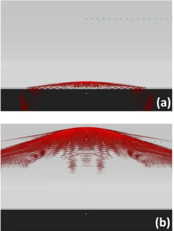
the coupledfluid-solid problem can be found in Komatitsch and Tromp [1999, 2002], Chaljub and Valette [2004], and Chaljub et al. [2007]. We used quadrilateral meshes, with Gauss-Legendre-Lobatto points and, for time discretization, we used finite difference scheme of Newmark of order 2. While the detailed results will be presented in a future paper (Khelfi et al., in preparation), Figure 7 demonstrates that thefirst arrival at distances not directly above the rupture zone may be, indeed, associated to the waves trapped in the ocean, which at ionospheric height appears as a head wave wavefront with a horizontal apparent speed directly associated to the hor-izontal speed of the waves trapped in the oceanic waveguide. [31] Our results show that coseismic TEC variations recorded
by satellites PRN27, PRN15, PRN09, PRN12, PRN18, PRN21, and PRN22 were not useful for imaging of the
seismic fault ruptured in the Tohoku-oki earthquake from the ionosphere. Analysis of geometry of GPS sounding for these satellites presents that they only could register propagation of coseismic perturbation, but not direct PAW, as in the case of PRN05 and PRN26. Apparently, ionospheric GPS detec-tion of the seismic source is only possible from observadetec-tions of those satellites and GPS receivers whose LOS cross the ion-osphere above the seismic region, as shown in Figure 3.
[32] Thus, despite the uncertainties in location provided by
the GPS sounding, our work demonstrates that GPS TEC mea-surements can be used for ionospheric detection of parameters of a seismic fault and rupture. And, therefore, ionospheric GPS measurements can be used for short-term tsunami warnings, either additionally to the currently working systems, or inde-pendent ionospherically based system might be developed in the future. Concerning the existing tsunami tracking methods, they nowadays rely on use of multiple instruments, such as seismometers, seafloor barometers, pressure gauges, ultrasonic wave gauges, moored GPS-mounted buoys, DART buoys, etc. Though that it works mostlyfine for smaller events, such mod-ern multiinstrumental approach proved to be able to fail under special circumstances as the M9.0 Tohoku-oki earthquake. When such a large quake occurs, the seismological data become saturated, which does not allow to estimate correctly the earthquake’s magnitude in short delays. Consequently, the expected tsunami wave heights can be underestimated, which may significantly increase a number of fatalities. Thus, in the case of large earthquakes and in the absence of possibility of near-real-time estimation of the moment magnitude, any ad-ditional rapid information on the seismic source is useful as it helps to correctly preview possible consequences of a seismic event. For instance, knowledge of seismic fault dimensions would provide information on the size of the initial displace-ments of the water column during a seismic event and the following tsunami generation, whereas knowing the position of the peak uplift would allow to approximately estimate the tsunami arrival time. However, undoubtedly, for developing a full method of near-real-time ionospheric detection of seis-mic/tsunamic source, further experimental studies and model-ing are necessary.
[33] Acknowledgments. This work was initiated under the support of the French National Research Agency (ANR, Project“To_EOS” ANR-11-JAPN-008), and was further developed andfinalized under the support of the European Research Council under the European Union’s Seventh Framework Program/ERC grant agreement n.307998. PL and KK thank the Office of Naval Research (Project “TWIST” N00014130035) for their support. We thank D. Komatitsch for SPECFM implementation and GENCI for the supercomputing supports. LR acknowledges the University of Nice for the support. We thank Geospatial Information Authority of Japan for the data of the GPS Earth Observation Network System (GEONET), National Geophysical Data Center (NGDC) for data of the Kokubunji ionosonde, and COSMIC CDAAC Data Analysis and Archival Center for the data of COSMIC satellite. We thank two reviewers whose comments helped to improve the manuscript. This is IPGP contribution 3435.
[34] Robert Lysak thanks David Galvan and Attila Komjathy for their assistance in evaluating this paper.
References
Afraimovich, E. L., N. P. Perevalova, A. V. Plotnikov, and A. M. Uralov (2001), The shock-acoustic waves generated by the earthquakes, Ann. Geophys., 19(4), 395–409.
Afraimovich, E., D. Feng, V. Kiryushkin, E. Astafyeva, S. Jin, and V. A. Sankov (2010), TEC response to the 2008 Wenchuan earthquake in comparison with other strong earthquakes, Int. J. Remote Sens., 31(13), 3601–3613, doi:10.1080/01431161003727747.
Figure 7. (a) Acoustic waves generated from an isotropic source located at depth of 19.5 km (orange cross), 100 s after the source reference time (the time of the earthquake, 05:46:23 UT). P velocities for the liquid and solid part are, respectively, 1.45 km/s and 5.8 km/s, while the shear velocity for the solid part is 3.2 km/s. The sound speeds in the atmo-sphere are those provided by model MSISE-00 [Picone et al., 2002]. The trapped waves in the ocean are clearly visible on both sides and are those generating the acoustic wave above the ocean. (b) Same simulation but for the moment 750 s af-ter the quake. The acoustic waves have reached an altitude of 300 km. Note a slight increase of the wavelength, associated to the larger sound speeds at this altitude. The wavefronts on both sides are those directly associated to the ocean reverber-ation and have therefore the same horizontal phase velocity, as most of the propagation in the ionosphere there is done with subvertical direction.
Astafyeva, E. I., and E. L. Afraimovich (2006), Long-distance propagation of traveling ionospheric disturbances caused by the great Sumatra-Andaman earthquake on 26 December 2004, Earth Planets Space, 58(N8), 1025–1031. Astafyeva, E., and K. Heki (2009), Dependence of waveform of near-field coseismic ionospheric disturbances on focal mechanisms, Earth Planets Space, 61, 939–943.
Astafyeva, E., K. Heki, V. Kiryushkin, E. L. Afraimovich, and S. Shalimov (2009), Two-mode long-distance propagation of coseismic ionosphere dis-turbances, J. Geophys. Res., 114, A10307, doi:10.1029/2008JA013853. Astafyeva, E., P. Lognonné, and L. Rolland (2011), First ionosphere images
for the seismic slip of the Tohoku-oki earthquake, Geophys. Res. Lett., 38, L22104, doi:10.1029/2011GL049623.
Bilitza, D., and B. Reinisch (2008), International Reference Ionosphere 2007: Improvements and new parameters, Adv. Space Res., 42(4), 599–609, doi:10.1016/j.asr.2007.07.048.
Calais, E., and J. B. Minster (1995), GPS detection of ionospheric perturba-tions following the January 17, 1994, Northridge earthquake, Geophys. Res. Lett., 22, 1045–1048, doi:10.1029/95GL00168.
Chaljub, E., and B. Valette (2004), Spectral element modelling of three-dimensional wave propagation in a self-gravitating Earth with an arbitrarily stratified outer core, Geophys. J. Int., 158, 131–141.
Chaljub, E., D. Komatitsch, J.-P. Vilotte, Y. Capdeville, B. Valette, and G. Festa (2007), Spectral element analysis in seismology, Adv. Geophys., 48, 365–419.
Ducic, V., J. Artru, and P. Lognonné (2003), Ionospheric remote sensing of the Denali earthquake Rayleigh waves, Geophys. Res. Lett., 30(18), 1951, doi:10.1029/2003GL017812.
Galvan, D., A. Komjathy, M. P. Hickey, P. Stephens, J. Snively, Y. T. Song, M. D. Butala, and A. J. Mannucci (2012), Ionospheric Signatures of Tohoku-Oki Tsunami of March 11, 2011: Model Comparisons Near the Epicenter, Radio Sci., 47, RS4003, doi:10.1029/2012RS005023. Hayes, G. P. (2011), Rapid source characterization of the 03-11-2011 Mw
9.0 Off the Pacific Coast of Tohoku Earthquake, Earth Planets Space, 63(N7), 529–534, doi:10.5047/eps.2011.05.012.
Heki, K., and J. Ping (2005), Directivity and apparent velocity of the coseismic ionospheric disturbances observed with a dense GPS array, Earth Planet. Sci. Lett., 236, 845–855, doi:10.1016/j.epsl.2005.06.010. Heki, K., Y. Otsuka, N. Choosakul, N. Hemmakorn, T. Komolmis, and
T. Maruyama (2006), Detection of ruptures of Andaman fault segments in the 2004 great Sumatra earthquake with coseismic ionospheric distur-bances, J. Geophys. Res., 111, B09313, doi:10.1029/2005JB004202. Hooper, A., J. Pietrzak, W. Simons, H. Cui, R. Riva, M. Naeije,
A. Terwisscha van Scheltinga, E. Schrama, G. Stelling, and A. Socquet (2013), Importance of horizontal seafloor motion on tsunami height for the 2011 Mw = 9.0 Tohoku-oki earthquake, Earth Planet. Sci. Lett., 361, 469–479.
Kherani, E. A., P. Lognonné, N. Kamath, F. Crespon, and R. Garcia (2009), Response of the ionosphere to the seismic triggered acoustic waves: elec-tron density and electromagneticfluctuations, Geophys. J. Int., 176, 1–13, doi:10.1111/j.1365-246X.2008.03818.x.
Kherani, E. A., P. Lognonné, H. Hebert, L. Rolland, E. Astafyeva, G. Occhipinti, P. Coisson, D. Walwer, and E. R. Paula (2012), Modelling of the Total Electronic Content and magneticfield anomalies generated by the 2011 Tohoku-oki tsunami and associated acoustic-gravity waves, Geophys. J. Int., 191(3), 1049–1066, doi:10.1111/j.1365-246X.2012.05617.x. Klobuchar, J. A. (1986), Ionospheric time-delay algorithm for single frequency
GPS users, IEEE Trans. Aerosp. Electron. Syst., AES, 23(3), 325–331. Komatitsch, D., and J. Tromp (1999), Introduction to the spectral-element
method for 3-D seismic wave propagation, Geophys. J. Int., 139(3), 806–822.
Komatitsch, D., and J. Tromp (2002), Spectral-element simulations of global seismic wave propagation. I Validation, Geophys. J. Int., 149(2), 390–412. Lastovicka, J., J. Base, F. Hruska, J. Chum, T.Šindelářová, J. Horálek, J. Zedník, and V. Krasnov (2010), Simultaneous infrasonic, seismic, mag-netic and ionospheric observations in an earthquake epicenter, J. Atmos. Sol. Terr. Phys., 72, 1231–1240.
Lay, T., Y. Yamazaki, C. J. Ammon, K. F. Cheung, and H. Kanamori (2011), The 2011 Mw 9.0 off the Pacific coast of Tohoku Earthquake: Comparison of deep-water tsunami signals withfinite-fault rupture model predictions, Earth Planets Space, 63, 797–801.
Liu, J.-Y., C.-H. Chen, C.-H. Lin, H.-F. Tsai, C.-H. Chen, and M. Kamogawa (2011), Ionospheric disturbances triggered by the 11 March 2011 M9.0 Tohoku earthquake, J. Geophys. Res., 116, A06319, doi:10.1029/2011JA016761.
Lognonné, P., J. Artru, R. Garcia, F. Crespon, V. Ducic, E. Jeansou, G. Occhipinti, J. Helbert, G. Moreaux, and P. Godet (2006), Ground-based GPS imaging of ionospheric post-seismic signal, Planet. Space Sci., 54, 528–540, doi:10.1016/j.pss.2005.10.021.
Makela, J. J., et al. (2011), Imaging and modeling the ionospheric airglow response over Hawaii to the tsunami generated by the Tohoku Earthquake of 11 March 2011, Geophys. Res. Lett., 38, L00G02, doi:10.1029/2011GL047860.
Maruyama, T., T. Tsugawa, H. Kato, M. Ishii, and M. Nishioka (2012), Rayleigh wave signatures in ionograms induced by strong earthquakes, J. Geophys. Res., 117, A08306, doi:10.1029/2012JA017952.
Occhipinti, G., P. Coisson, J. J. Makela, S. Alleyger, A. Kherani, H. Hébert, and P. Lognonné (2011), Three-dimensional numerical modeling of tsunami-related internal gravity waves in the Hawaiian atmosphere, Earth Planets Space, 63, 847–851.
Occhipinti, G., L. Rolland, P. Lognonné, and S. Watada (2013), From Sumatra 2004 to Tohoku-Oki 2011: the systematic GPS detection of the ionospheric signature induced by tsunamigenic earthquakes, J. Geophys. Res. Space Physics, 118, 3626–3636, doi:10.1002/jgra.50322.
Okada, Y. (1992), Internal deformation due to shear and tensile faults in a half-space, Bull. Seismol. Soc. Am., 82, 1018–1040.
Picone, J. M., A. E. Hedin, D. P. Drob, and A. C. Aikin (2002), NRLMSISE-00 empirical model of the atmosphere: Statistical comparisons and scientific issues, J. Geophys. Res., 107(A12), 1468, doi:10.1029/2002JA009430. Rolland, L., G. Occhipinti, P. Lognonné, and A. Lovenbruck (2010),
Ionospheric gravity waves detected offshore Hawaii after tsunamis, Geophys. Res. Lett., 37, L17101, doi:10.1029/2010GL0444479. Rolland, L., P. Lognonné, and H. Munekane (2011a), Detection and
model-ing of Rayleigh wave induced patterns in the ionosphere, J. Geophys. Res., 116, A05320, doi:10.1029/2010JA016060.
Rolland, L., P. Lognonné, E. Astafyeva, A. Kherani, N. Kobayashi, M. Mann, and H. Munekane (2011b), The resonant response of the iono-sphere imaged after the 2011 Tohoku-Oki earthquake, Earth Planets Space, 63(7), 853–857, doi:10.5047/eps.2011.06.020.
Rolland, L. M., M. Vergnolle, J.-M. Nocquet, A. Sladen, J.-X. Dessa, F. Tavakoli, H. R. Nankali, and F. Cappa (2013), Discriminating the tectonic and non-tectonic contributions in the ionospheric signature of the 2011, Mw7.1, dip-slip Van earthquake, Eastern Turkey, Geophys. Res. Lett., 40, 2518–2522, doi:10.1002/grl.50544.
Romano, F., A. Piatanesi, S. Lorito, N. D’Agostino, K. Hirata, S. Atzori, Y. Yamazaki, and M. Cocco (2012), Clues from joint inversion of tsunami and geodetic data of the 2011 Tohoku-oki earthquake, Sci. Rep., 2, 385, doi:10.1038/srep00385.
Simons, M., et al. (2011), The 2011 Magnitude 9.0 Tohoku-Oki Earthquake: Mosaicking the Megathrust from Seconds to Centuries, Science, 332(6036), 1421–1425, doi:10.1126/science.120673.