3-D optical waveguide arrays for in-vivo optogenetics : development and application

3-D Optical Waveguide Arrays for In-Vivo Optogenetics:

Development and Application

by

Anthony N. Zorzos

S.M., Department of Aeronautics and Astronautics, Massachusetts Institute of Technology, 2009 Sc.B., Applied Physics, Brown University, 2007

Submitted to the Program in Media Arts and Sciences, School of Architecture and Planning, in partial fulfillment of the requirements for the degree of

Doctor of Philosophy in Media Arts and Sciences at the

MASSACHUSETTS INSTITUTE OF TECHNOLOGY

June 2013

MASSACHUSTT INS E OF TECHNOOGY

JUL 19 2013

LIBRARIES

This work is licensed under a Creative Commons Attribution 3.0 Unported License The author hereby grants to MIT permission to reproduce and distribute publicly paper and

electronic copies of this thesis document in whole or in part.

Author

Anthony N. Zorzos Program in MediaAsn

--- _{May, 2013}

Certified by

Prof. Edward S. Boyden Leader, Synthetic Neurobiology Group Associate Professor, MIT Media Lab and McGovern Institute, Departments of Biological Engineering and Brain and Cognitive Sciences

Accepted by

Prof. Patricia Maes Associate Academic Head Program in Media Arts and Sciences

3-D Optical Waveguide Arrays for In-Vivo Optogenetics:

Development and Application

by

Anthony N. Zorzos

Submitted to the Program in Media Arts and Sciences, School of Architecture and Planning, on May 24, 2013, in partial fulfillment of the requirements for the degree of Doctor of Philosophy in Media Arts and Sciences

Abstract

A key feature of neural circuits in the mammalian brain is their 3-dimensional geometric complexity. The ability to optically drive or silence sets of neurons distributed throughout complexly shaped brain circuits, in a temporally precise fashion, would enable analysis of how sets of neurons in different parts of the circuit work together to achieve specific neural codes, circuit dynamics, and behaviors. It could also enable new prototype neural control prosthetics capable of entering

information into the brain in a high-bandwidth, cell-specific fashion. This dissertation work involves the development, characterization, and initial utilization of a technology capable of delivering patterned light to 3D targets in neural tissue.

Silicon oxynitride waveguide fabrication was optimized for integration onto insertable silicon probes. The waveguides have a propagation loss of-0.4 dB/cm. Right-angle corner mirrors were fabricated at the outputs of the waveguides with losses measured to be 1.5 ± 0.4 dB.

Silicon MEMS techniques were developed to fabricate both single- and multi-shank probe geometries with integrated waveguides. Methods were developed to assemble the multi-shank probes into a 3D format using discrete monolithic silicon pieces.

Three coupling schemes were developed to couple light to both single- and multi-shank probes. For individual probes not assembled in a 3D format, ribbon cables were used. Modular connection schemes were developed based on ribbon cable connector technologies. Input coupling losses were measured to be 3.4 ± 2.2 dB. For probes which were assembled in a 3D format, two coupling

methods were developed: projector-based and scanning-mirror-based. The losses associated with the projector-based system are 17.3 ± 1.8 dB. With a 1.5W 473 nm laser source, 100 pW is capable of being delivered from 300 separate waveguides. The losses associated with the scanning-mirror-based system are 11.9 ± 2.5 dB. With a 1.6 mW 473 nm laser source, 100 pW is capable of being delivered from an individual waveguide.

These fabrication, assembly, and coupling methods demonstrate a successful development of a technology capable of delivering patterned light to 3D targets in neural tissue. Initial biological experiments being performed on microbial-opsin expressing mice is presented. 3D patterned light is delivered to targets in the primary somatosensory cortex while electrical activity is recorded from the primary motor cortex.

Thesis Supervisor: Professor Edward S. Boyden

Title: Associate Professor, MIT Media Lab and McGovern Institute, Departments of Biological Engineering and Brain and Cognitive Sciences

3-D Optical Waveguide Arrays for In-Vivo Optogenetics:

Development and Application

by

Anthony N. Zorzos

The following people will serve as readers for this thesis:

Thesis Reader

Clifton G. Fonstad Leader, Compound Semiconductor Research Group Vitesse Professor of Electrical Engineering

Thesis Reader

Ramesh Raskar Leader, Camera Culture Group Associate Professor of Media Arts and Sciences

Acknowledgements

I would like to take this space to acknowledge and thank all the people who have been such help and support over my time as a doctoral student.

First, I'd like to thank Professor Raskar for agreeing to be a committee member and thesis reader. He has provided very helpful feedback during the project development and the writing of this dissertation. Furthermore, in interacting with him and his students over the last few years on separate projects has proven very beneficial. Next, I'd like to thank all the members of the Boyden Lab. They have proven to not only be excellent resources for knowledge and support, but also a fun group to spend time with.

I'd also like to acknowledge all the help and support I've gotten over the years from the MTL research staff. I'd especially like to mention Dennis Ward, Kurt Broderick, Donal Jameison, Eric Lim, Paudely Zamora, Paul Tierney, and Vicky Diadiuk. They all drilled into me a practical and theoretical understanding of micro-fabrication methods, and for that I am deeply grateful.

There are three labmates I'd like to select out as having been especially supportive and helpful. First, to Dr. Justin Kinney I'd like to say it would be haaaardaaaa to find someone so able to balance intellectual brilliance, clarifying lucidity, and such a vulgar

sense of humor: thank you. Next, to the intellectual heavy-weight Dr. Tim Buschman I'd like to say you have given me a first-hand glimpse into the world of neuroscience and the most sublimely humorous form of egotism: thank you. Finally, to Dr. Jorg Scholvin, you

have been more a mentor and guide than a labmate, and are brilliant enough to have made me feel like an idiot for three straight years: thank you. To all three of you: thank you.

The most important two figures during my time as a PhD student have been my co-advisors Professor Fonstad and Professor Boyden. I cannot thank you enough for your generosity, your time, your brilliance, your patience, your kindness, and your guidance. I feel deeply honored to have been so closely followed by such outstanding advisors. I have learned so very much over the last four years and look forward to maintaining our

relationship for years to come. More importantly than passing to me intellectual material, you have been ideal role-models for character and conduct both as academics and human beings.

Finally, I want to thank a few close friends who have truly helped me over the years: Dan Courtney, Paulo Lozano, John Churchill, Chad Gilette, Josh Bartok, and Lama Willa Miller: thank you, thank you, thank you! My Smakula in-laws, my cousins, my aunts, my uncles, my Yiayia and Pappou. My sister, her husband, and my dearest, dearest nephew

Stevie. To my parents, Steven and Pauline Zorzos, the father and the mother, the fire and the anvil, the upward and the downward, the outward and the inward, the becoming and the being, the freedom and the fullness: thank you!

Most importantly, I want express my Gratitude and Love for my wife, Kathleen Zorzos: you are my Heart.

Contents

3.1 On-chip W aveguide Fabrication Background... 59

3.2 W aveguide Fabrication... 63

3.3 W aveguide Characterization ... 71

4.1 Single-shank Probe Fabrication ... 82

4.2 M ulti-shank Probe Fabrication ... 88

4.3 Assembly of Multi-shank Probes for 3D Illumination ... 90

5. Methods for Coupling Light Into Assembled Arrays ... 97

5.1 Introduction to Chapter ... 97

5.2 Illum ination Requirem ents... 98

5.3 Delivery of Light to Array...101

5.3.1 Ribbon Fiber ... 101

5.3.2 Scanning M irror Galvanometer System ... 104

5.3.3 Digital M icro-mirror Device System ... 107

5.4 Imaging Fiber Bundles ... 115

5.5 Alternatives to Imaging Fiber Bundles ... 118

6. Conclusion ... 121

6.1 Prelim inary Biological Experiments...121

6.1.1 Motivation... 121

6.1.2 Experimental Setup ... 123

6.1.3 Pre-processing ... 128

6.2 .1 Sum m ary ... 13 2

6.2.2 Recommendations and Future Directions... 134

Appendix A: Detailed Fabrication Flow for On-chip W aveguides...138

Appendix B: Detailed Fabrication Flow for Light-proof Electrodes...141

Appendix C: Experimental SOP for Preliminary Biological Experiments...145

Appendix D: Light-proof Electrodes... 153

Chapter 1: Introduction

1.1 Background

This doctoral work is motivated by a fundamental question in systems neuroscience: how do sets of neurons in different parts of the brain work together to achieve specific neural codes, circuit dynamics, and behaviors? The scale of modem research addressing this single general question is large (Buzsaiki, 2006; Engel, Fries, & Singer, 2001; Miller & Buschman, 2013; Rieke, 1997). This dissertation provides a particular tool representing a contribution to systems neuroscience, whereby large-scale optogenetic 3D neural mapping becomes a possibility. Furthermore, this dissertation will extend beyond the development of the technology into its preliminary scientific utilization for mapping large-scale cortical networks.

Systems neuroscience is the study of how neural networks communicate and give rise to neural dynamics and behavior. The brain has a large number of neurons (-75 million

in a mouse, -2 billion in a chimpanzee, and ~85 billion in a human) (Kandel, 2012). The complexity of these systems, directly related to the scale of the neural networks studied, is large. It is desirable, in approaching such a complex problem, to be equipped with the necessary technologies capable of teasing out the dynamics and relationships arising within said networks.

There are many different types of neural technologies, i.e. technologies seeking to address fundamental neuroscientific questions as well as potentially treat neuropathologies, (DiLorenzo & Bronzino, 2008; Frontiers Research Foundation., 2008; Katz, 2008; Maurits, 2012; Michael & Borland, 2007). These technologies include electrophysiological

technologies (e.g. microelectrode arrays, patch clamping, etc.), neural imaging technologies (e.g. functional magnetic resonance imaging, magneto encephalography, etc.), drug delivery techniques technologies, etc.

This thesis develops a technology capable of affecting neural activity with resolution in space (i.e. many points in a volume of tissue), time (i.e. fast temporal dynamics), polarity (i.e. activate or deactivate neurons), and type (i.e. address different classes of neurons independently). The new field of optogenetics provides an optimal platform from which to develop such a technology.

Optogenetics enables the ability to delivery light into the brain for the purposes of controlling neural activity and other biological processes. As the name suggests,

optogenetics involves the genetic manipulation of neural tissue so that it is subsequently made light-sensitive (i.e. can be controlled on the millisecond timescale with photonic

precise activation or deactivation of cellular activity. Cell-type resolution is accomplished through the use of specific targeting mechanisms. The microbial opsins most commonly used are channelrhodopsins (Boyden, Zhang, Bamberg, Nagel, & Deisseroth, 2005),

halorhodopsins (Han & Boyden, 2007; F. Zhang, Wang, et al., 2007), and archaerhodopsins (Chow et al., 2010; Han et al., 2011). See Figure 1.

A B C

archaerhodopsins and habrhodopoins channeirhodopsins

bacterirhodopsins (e.g., HaloMpHR) (e.g., ChR2)

(e.g., Arch, Mac, BR) _{W NO% 1. e}

"AftL____A__1

MINL

111111

_"'liz

Figure 1 - (A) The archaerhodopsins and bacteriorhodopsins are light-driven outward proton pumps. (B) The halorhodopsins are driven inward chloride pumps. (C) The channelrhodopsins are

light-gated inward nonspecific cation channels. Adapted from (Boyden, 2011)

As shown in Figure 1, the channelrhodopsins are light-gated inward nonspecific cation channels, the halorhodopsins are light-driven inward chloride pumps, and the

archaerhodopsins/bacteriorhodopsins are light-driven outward proton pumps. Getting these microbial opsins to express in the cell membrane is an area of active research and

development in molecular biology (Madisen et al., 2012). Strategies have largely involved cell-specific promoters and customized viruses for genetic targeting. There is also a

growing use of germline transgenesis for permanent gene transfer. These 'transgenic mice', as they will be referred to throughout this work, avoid many of the costs and difficulties

associated with using viruses for opsin expression. Both expression methods are used in this work.

Structured illumination across the 2D surface of cortex has been used previously (Sakai, Ueno, Ishizuka, & Yawo, 2013) (Figure 2). As powerful as this approach may be, it is inherently limited by the 2D nature of the light delivery. Deep neural targets are

impossible to reach given the opacity and optical properties of brain tissue (Johansson, 2010). Microscope DMD objecove lens specid

Figure 2 - DMD-based projector system used to project arbitrary 2D geometries onto cortex surface (Sakai et al., 2013). The LED is a light emitting diode array for DMD (digital micromirror device)

illumination. The DMD is used to sculpt the light in arbitrary 2D patterns to be projected.

There is also work being done on adapting the technology of two-photon microscopy to

optogenetics for stimulation at-depth (Oron, Papagiakoumou, Anselmi, & Emiliani, 2012). Two-photon microscopy, relying on two-photon absorption by fluorophores, is an imaging technique used to image tissue at depth. In adapting this technology for optogenetics,

limited to a depth of 1 I mm. Although it can be used to illuminate different regions of a 3D space, it cannot provide illumination to arbitrary 3D geometries.

To date, numerous in vivo studies have used optical fibers to deliver visible light into brain targets in which neurons express opsins, but an optical fiber can target just a single region (Figure 3). Beyond simple light delivery, individual optical fibers have been adopted to use in complex behavioral experiments (Aravanis et al., 2007; Gradinaru, Mogri,

Thompson, Henderson, & Deisseroth, 2009). Technologies have also been developed to avoid the use of optical fiber tethering altogether using wireless LED sources (Wentz et al., 2011). An implantable probe capable of delivering light to arbitrary points in a

3-dimensional volume would enable more versatile optical control, opening up the ability to deliver patterned light to manipulate neural activity in distributed brain circuits.

a Optical fibre

Cannula

Cranioplastic cement Skull

Illumination

Figure 3 - The majority of optogenetics experiments to-date have involved single optical-fiber stimulation, adapted from (F. Zhang, Aravanis, Adamantidis, de Lecea, & Deisseroth, 2007). (a) is a

schematic of a how a single optical fiber is usually implanted and attached to the skull. (b) shows a mouse, freely-moving, with a single optical fiber implanted.

Although a natural first step for optogenetics-based experiments, individual fibers do not allow for easily scaling to hundreds/thousands of individual deliveiy sites. This dissertation does not move away from the fundamental technology of fiber-optics, but utilizes the

developments of integrated photonics and on-chip waveguide fabrication as a framework for fiber-optic miniaturization and scaling.

1.2 Overview

This dissertation presents and characterizes a technology, based on the advancements of integrated photonics, allowing for the delivery of illumination to arbitrary 3D geometries in brain tissue. Light is coupled from an external source to fiber optics which terminate at different depths along an array of implantable shanks.

Chapter 2 will present general theoretical considerations behind the technology. Specifically, the theory behind optical waveguides is presented, for both single-mode and multi-mode fiber optics. The coupling efficiency between separate waveguides is presented. Evanescent coupling and micro-bending loss, largely influencing packing density (of

waveguides), is also discussed. Finally, the issue of heating neural tissue is discussed, an important theoretical consideration when choosing to use waveguides instead of direct source implantation.

In Chapter 3, the process of waveguide fabrication is presented. The waveguide loss characterization is shown and the different mechanisms discussed. The characterization allows for the fabrication of single-shank and multi-shank waveguide probes with minimal

size and subsequent tissue damage. These single- and multi-shank probe geometries are shown and characterized.

Chapter 4 describes the fabrication procedure and methods used to assemble multi-shank probes into full 3D probe arrays. The chapter also offers a characterization of how these assembly methods affect the geometrical alignment of the multi-shank probes.

Chapter 5 is a description of the different coupling methods used for the 3D probe arrays: a DMD-based system and a scanning galvanometer-based system. The loss mechanisms of the two systems are characterized, and a critique of the two systems is offered based on the performance results.

Chapter 6 is a conclusion chapter. This chapter both summarizes the developed technology and its performance, as well as provides an in-depth description as to how this technology can be improved and where it can lead to in terms of new research avenues. There is also a discussion of preliminary biological experiments being conducted.

Appendix A is a detailed process flow for the fabrication of on-chip waveguides. Appendix B is a detailed process flow for the fabrication of light-proof electrodes. Appendix C is the standard operating procedure for preliminary biological experiments. Appendix D is a description of work done on light-proof electrodes.

Chapter 2: Theoretical Considerations

The developed technology maintains the light source outside of the neural tissue (to mitigate heating issues) and guides the light along waveguides to deep neural targets. In this chapter, the basic theory of waveguide operation is developed and discussed, with emphasis given to planar dielectric waveguides. First fiber optics in general will be discussed. Then, planar dielectric waveguides followed by an extension to two-dimensional waveguides. Following this, the coupling efficiencies, propagation losses, micro-bending losses, and heating will be discussed. Heating of neural tissue is a particularly important consideration and the discussion in this chapter will clearly and quantitatively explain why optical

2.1 Fiber Optics

2.1.1 Electromagnetic Theory

Optical waveguides can be categorized by several classifiers: mode structure (single-mode, multi-mode), index profile (step, gradient), geometry (slab, strip, fiber), and material (glass, polymer, semiconductor). This section will seek to develop the theory behind a fiber-based geometry. Fiber waveguides are usually cylindrical in geometry (Figure 4) and are composed of a dielectric central core surrounded by an outer cladding. The core dielectric has a higher index of refraction relative to the cladding material. Speaking from a

perspective of ray-based optics, light incident on the core/cladding boundary at angles greater than the critical angle (to be defined below) are totally internally reflected, and therefore 'guided' by the fiber. In the interest of completeness, this discussion of fiber optics will begin with a wave-based perspective and then lead us into the ray-based perspective when dealing with planar waveguides.

Cladding Light ray

Figure 4 - Cylindrical dielectric step index waveguide, where 2a is the core diameter. (PhotonicsOnline)

dE V x H = E ~-a V x E = -#0 _a V -E 0 V-E=0 V-H = 0,

where E and H are the electric field and magnetic field respectively, and the constants so and

po are the electric permittivity and magnetic permeability respectively. The electric field

and magnetic field, forming an electromagnetic wave, must satisfy the above coupled set of differential equations. For E and H to satisfy Maxwell's equations, it is necessary that each of their components (E, Ey, E, H, H, Hz) satisfy the wave equation,

1 a2u c02 at 2_' where 1 Co E0

9

is the speed of light in vacuum. As mentioned, this set of coupled differential equations govern electromagnetic waves in free-space. Dielectric waveguides involve the propagation of light in a medium, so Maxwell's equations must be adjusted accordingly. Maxwell's equations in a medium (source-free) become,

aD

VxH=-B

V - B = 0,

where D is the electric flux density, B is the magnetic flux density, and both depend on the properties of the medium of propagation. Specifically,

D = E0E + P

B = poMH + poM

where P is the polarization density (expressing the density of electric dipole moments in a dielectric material) and Mis the magnetization density (expressing the density of magnetic dipole moments in a magnetic material). The magnetization density can be assumed for this discussion to be zero, as any and all media addressed here are non-magnetic. If we assume a time-harmonic field with time dependence e-iw, where oz=2xv is the angular frequency, then Maxwell's equations become,

V x H =

joD

V x E = -jB V-D=0

V- B = 0.

The time-harmonic field with time dependence is a safe assumption given the condition that the electromagnetic wave under analysis is monochromatic. For the purposes of this work,

the simplest case to consider (linear, nondispersive, homogeneous, and isotropic media) will be sufficient. Given this case, the vectors P and E are related as,

P = EoXE,

where

x

V x H =jweE V X E = -jwyoH V-E=0

V H =0.

Because E and H satisfy the wave equation (above), all components of E and H (represented by U(r)) must satisfy the Helmholtz equation,

V2_{U + k}2

U = 0,

where k = o Y = nko, n is the refractive index, and ko = w/co.

Using this developed electromagnetic theory, we can now look at how

monochromatic light propagates in step-index fibers. As shown previously, each of the electric field and magnetic field components must satisfy the Helmholtz equation, where

n=n1 in the core and the index of refraction is n2 in cladding (Figure 5). The cladding

thickness is assumed to be of infinite extent. In a cylindrical coordinate system, the Helmholtz equation becomes,

a2U 1aU 1 2U a2U

+r + + + n2ko2_U=O0

r rar r289 azz

The solutions to this equation will take the form of waves traveling in the z direction with propagation constant

p.

CLADDING

Figure 5 -Basic schematic of fiber showing geometric parameters. The cladding is taken as infinite in extent.

U must be a periodic function in p, so we can substitute the separated equation, U(r, 'p, z) = u(r)e-il'Pe -jz, 1 = 0, ±1, ±2, ....

into the above cylindrical-form of the Helmholtz equation to get the following ordinary differential equation for u(r),

d2u 1du 22

+ -+ (nzk2 _ u 0.

dr2 _{rdr r}

The wave is bound (or guided) by the fiber if the propagation constant,

P,

d'u+ 1du+ kT2 _{u12 =0, r <a (core)} dr2 r dr r2 ) dzu 1du

(

where kT2 _{= ni2ko}2 _{- f2, and y}2 _fl2 _{- n}

22ko

2_{. For guided waves kT}2 _{and y}2 _are

positive and kT and y are real. Bessel functions are the solutions to the above differential equations. Specifically, we have,

u (r) oc

J

These solutions, or 'modes', represent the set of possible cross-sectional field profiles in a fiber (given the set of constraints utilized in the refinement of Maxwell's equations). The cladding solution, Ki (yr), a modified Bessel function of the second kind and order 1, represents the evanescent penetration of the given mode into the cladding (Figure 6).

! \I I I 0.8 - J0- ~Du KJW~-- --0.6 - 2.5 - .U 0.4 -2V0 0.2 . 0.0 IV. _____ -0.20--0.4 - 0.0 -_____ X X

Figure 6 - Solutions to the Helmholtz equation for both the core (left) and cladding (right). The solution for the core is a Bessel function of the first kind, and the solution for the cladding is a modified Bessel

If we normalize the parameters kT and y by the fiber core radius, a, then we can define what is known as the V-number,

V2 _{= a2(kr} 2

+ y2).

Plugging in the defined values of kT and y, we see that V is a conserved quantity,

V = 271-a(n 2 _n 22)1/2 = 2w- aNA.

This is an important parameter to define in classifying a fiber as single-mode or multi-mode, a consideration which we will return to later in this work. Recalling the substituted relation for the components of E and H,

U(r, p, z) = u(r)e -me -jflz, m = 0, 1, i2, . 1 = 0, +1, +2,

we now have a spatial profile, for any given location z, in terms of r and <. The different modes are usually denoted LPl,n. A graphic showing a small number of the different modes and their corresponding amplitude profiles (for a fiber with a V-number of ~12) is shown in Figure 7 below (Paschotta, 2011).

LP$ LPr, 7 6 * iA 2 13. e #A I* Z LCP3 LP LL 3 23*4 mod ne, m LPOI _LU2L, L0 2 moxde index mn

Figure 7 -LP modes for a step-index cylindrical optical fiber (Paschotta, 2011). The different colors represent different polarity electric field solutions. How many modes are supported by an individual optical fiber depends on the light wavelength and fiber characteristics (size and indices of core and

cladding).

How many modes are supported by an individual optical fiber depends on the wavelength of interest and fiber characteristics (size and refractive indices of core and cladding

respectively). This is reflected in the V-number defined above. Note that there are discrete modes, i.e. not a continuum of solutions, because the eigen-solutions to the Helmholtz equation are discrete (above).

2.1.2 Ray-Based Theory

Now that a basic wave and electromagnetics-based understanding and theory of fiber optics have been established, the more specific case of planar dielectric waveguides can be addressed. Because planar waveguides, defined by their geometry, do not have a rotational symmetry like fiber waveguides (cylindrical), the Maxwell-based solutions are significantly more complex. It is for this reason a ray-based approach is usually utilized to derive

waveguide modes, number of modes, field distributions, etc. for planar waveguides.

Considering first a 2-D condensation (slab waveguide) of the 3-D general case, we first look at the internal field distribution (the field distribution in the core material (Figure 8)).

n2

Z

Figure 8 - Slab dielectric waveguide with two separate refractive indices.

As the more-fundamental and complete electromagnetics discussion has already been made with regards to cylindrical fiber optics (above), we can here skip the detailed ray-based and less fundamental derivation of the transverse electric-field amplitude (Saleh & Teich, 2007),

Ex(y, z) = amum(y) exp(-jflz), where

#m

before), a,, is a constant,

Cos _{y27 m ,i =) 0,2,4,}

... _{d d}

Um(Y) 0C sn my(sn-,

--sin 2r --sin 6m 1 2 2

and k=ko/ni. In the derivation of this transverse field, 0m is the angle of the TEM plane wave incident in the slab waveguide. As with the electromagnetics-based derivation, there are discrete solutions reflecting discrete modes. In this ray-based derivation, the included solutions are those which do not result in the necessary path lengths for destructive

interference (Kasap, 2013). For the external field (the field distribution in the cladding), we have, ( d e-Ymyy Y _ Um(Y) 0C 2 e-rmyy Y _ 2 The extinction coefficient, Yn, can be defined as,

Cos20

Ym = nzko _COS_ 2 _g .- 1,

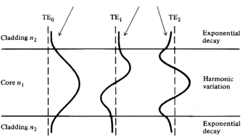
TEO _TE, Cladding n₂ TE₂ I Exponential T1 decay Core n Harmonic variation Claddingn2 II Exponential n 1decay n2

Figure 9 - Transverse electric-field amplitude for several ID dielectric slab waveguide modes (Keiser, 2011).

As with the electromagnetics-based derivation for a cylindrical optical fiber, the number of modes possible depends on the numerical aperture, the wavelength, and the size of the fiber. Increasing the core radius or refractive index increases the number of modes, while

increasing the wavelength or cladding refractive index lowers the number of modes. As the number of possible modes drops to 1, the optical waveguide becomes a single-mode fiber, i.e. it can only sustain the fundamental mode. For instance, by decreasing the core radius, the number of modes decreases. At some radius, only the fundamental mode can be

sustained. The core can be decreased in size even further while sustaining the fundamental mode, however the evanescent penetration will increase in the cladding.

Note that as the mode number, m, increases, the extinction coefficient decreases, yielding an evanescent wave with longer spatial penetration into the cladding. This is

confinement to a maximum and want to avoid evanescent coupling (into either the substrate or neighboring waveguides).

2.1.3 Coupling

There are many methods for coupling light to a waveguide, either from a light source or another waveguide (Hunsperger, 1991). These methods include free-space coupling, butt-coupling, and diffraction-coupling, to name a few (Figure 10).

Inckent Prism Uight

Figure 10 - Examples of various coupling methods: butt coupling (upper left), diffraction coupling (upper right), and prism coupling (bottom).

Briefly, as has been previously discussed, the optical field spatial profile is a superposition of modes,

E(y, z) = _{amum(y)e -jmz,}

where m is representative of the mode 'number' (symbols defined in previous section). The relative composition of this superposition depends on the light source used to 'excite' each mode. We can write that for a source of arbitrary distribution, s(y), the amplitude of each excited mode g, is,

ag = fs(y)ug(y)dy.

This amplitude coefficient, ag, is representative of the 'overlap' between the source

distribution and the mode of interest. As will be further described in Chapters 3 and 5, the chosen method of coupling is butt-coupling from a fiber-optic source. Furthermore, the input fiber is a single-mode fiber. Therefore, the 0th mode is the primary mode being excited for the final fiber arrays, yet to be described. There is the possibility of what is known as upward mode coupling. This involves the transfer of power between modes of lower order to modes of higher order. This can occur in any number of ways, including micro-bending and scattering events. So, even though initial coupling might excite predominantly the fundamental mode, the higher modes of the fabricated fiber can still be utilized.

As was already alluded to, evanescent penetration is a potential problem in the design constraints. In the case of evanescent penetration into substrate (higher index material), that results in what is known as evanescent loss. In the case of evanescent

penetration into a neighboring waveguide (equal index to core, and, more importantly, a lower index than the cladding), that results in what is known as evanescent coupling. Even though evanescent coupling does not, theoretically, involve the loss of power, in this case it can be treated as such. This will be directly addressed in Chapter 4.

2.1.4 Bend Loss

As briefly described in the introduction, the goal of the technology developed is to

deliver light laterally along the length of an insertable shank. Although not the only conceivable method, the approach taken is to redirect the propagating light 90' relative to the direction of insertion. Redirecting optical waveguides at right angles is an important

area of research in integrated photonics (Espinola, Ahmad, Pizzuto, Steel, & Osgood, 2001; Lin, Lin, Chen, & Li, 2009). Specifically, the important question is how to create optical waveguides with 90' low-loss small radius-of-curvature bends. This is important because

the smaller the radius of curvature (for some given allowable loss), the higher the available packing density for optical interconnects.

An intuitive analytical approach for addressing the minimum bend radius involves

the radiation caustic. Consider the phase front of a fundamental mode propagating through

core

Figure 11 -Phase front for the fundamental mode in a bent slab waveguide

The angular velocity of the phase front, relative to the center (C), is taken to be Q. The phase velocity at the beginning of the bend must be equal to the phase velocity at the end of the straight input section,

(0

Rbf2 =-W

where o is the frequency, and

P is the propagation coefficient. Solving for 92 and

p,

C

f = Rbneff'

where c is the speed of light in vacuum, and neff is the effective index of the fundamental mode. A radius, Rrad, is defined as the radius, relative to C, at which the phase velocity of the wave front equals the speed of light in the cladding,

C DQRrad

=n---ncl

Rraa =leff Rb. ncl

As the phase velocity in the cladding cannot exceed the speed of light in the cladding, at

Rrad, the penetrating evanescent tail radiates into the cladding. This interface is the radiation caustic. Because the evanescent tail is has an exponential decay, there is always some

radiated power for any given bend radius. However, as Rb decreases, Rrad becomes smaller and smaller, leading to an increase in bend loss. It should also be noted that this relation also holds for higher-order modes. However, as was shown in the previous sub-section, the evanescent penetration into the cladding is larger for higher-order modes. Therefore, the bend loss is even more severe for higher-order modes. Another way of seeing this is that the effective index for higher order modes is lower, meaning Rrad is smaller and subsequently

more bend loss. Therefore, for a given waveguide structure, the least bend loss occurs for the fundamental mode and the most bend loss occurs for the highest-order modes.

The theoretical bend loss for a given fiber optic was worked out by Dietrich Marcuse in 1976 (Marcuse, 1976),

rep 1/2 y2W1/2 4 Rb W]

Y RbJ 2pU2 ex 3 p V2

where y is related to the bend loss by P(z) = P(0)e-yz. P(z) is the power at any given point along the bend, P(O) is the power at the beginning of the bend, z is the distance along the bend, and y is defined above. Rb is the bend radius, p is the waveguide diameter

(cylindrical geometry assumed), A= ,co-c nco is the core index of refraction, ner is the

cladding index of refraction, the V-number is previously defined, and U, as well as W, are modal parameters elsewhere defined in terms of fiber characteristics (Saleh & Teich, 2007),

U = kp(neO 2

_ neff 2

W = kp(neff 2

_ n 2_)f

By substituting the modal parameters into the Marcuse bend-loss relation, an analytic equation relating bend loss to bend radius is derived (derivation not shown),

1 1 3

P1 fTk 'zi (nco - ncl)nco(neff 2 - ncl2) (neff 2 _ 2) (iRb

This is specifically derived for a right-angle, hence the rRb/4 term in place of z. With this

analytical relation, the bend radius can be solved for any given power loss. The following figure is a plot of the bend radius of curvature as a function of core index for several

throughputs (50%, 60%, 70%, and 90%). The cladding index is held at 1.46. Note, this plot is for the fundamental mode, and therefore is an optimistic estimate of bend loss. Higher order modes will require even larger bend radii for the same loss.

104 10 e 10, 0 E 102 LL 2 10 10 Core Index

Figure 12 -Bend radius of curvature for a right-angle bend as a function of core index for several throughputs. The cladding index is held at 1.46.

This is an important calculation to make because the packing density must be made as high as possible. Figure 13 is a schematic illustrating why the bend radius is such an important consideration. ... ... ...- ... ..-*. .... .. ...5 0%.. .. ......... ... ...- ... .. ... ....I . 6 0%.. .. ... .. . ... _{.. ..} . .. .. .. _{.. .... ... .. .. ...} . .. .. .. _.- .. . .. .. .. . . -- - -- .- 7 0 % -9 0%.. .. . .... .......... .... - -...... ...... 1. .. . ... I 1 . . . .... 1.7. .1.. . 8...1 .9.. .. ..

Figure 13 - The distance between the outermost waveguide and the substrate edge is at least the bend radius in length.

The distance between the outermost waveguide and the edge of the substrate is at least the radius of curvature for the 90' bend. This is an extremely important consideration for a this technology because the larger the size of the inserted shank, the more damage is done to the tissue. Keeping the size of the shank at an absolute minimum is paramount. For reasons which will be discussed in greater detail in the next chapter, the silicon oxynitride film deposited cannot go above an index of ~1.6. This has to do with the scattering and

absorption properties of the silicon oxynitride films when there is a large nitride content. As can be seen from the theoretical work summarized in Figure 12, the bend radius must be at least ~50 iim for a loss of 80%. Also, this is for the fundamental mode, and therefore is a best-case scenario. Higher modes will have even higher losses.

The method taken to avoid this problem entirely is through the use of local mirrors. At the point in the waveguide when the right angle is to be introduced, a sharp 900 bend is

introduced. The 90' bend does not allow for mode confinement. In fact, based on the theory developed above, even the fundamental mode is not confined. So, regardless of whether the waveguide is single-mode or multi-mode, all modes are upward coupled to

radiation modes. The light, no longer confined to the core, is reflected off of a local mirrored surface at the abrupt junction (see Figure 14).

Minimal additional substrate width Waveguide outputs _{_} Optical waveguides Highly-reflective mirrored-surfaces

Figure 14 - Right-angle highly-reflective mirrored surfaces provide a way to avoid the unwanted extra space necessary in maintaining mode confinement in 90* curved bends.

The minimum additional substrate width is -5 ptm given the tolerances of deep RIE silicon etching. The reason the outputs are wider than the optical waveguide main body will be discussed in subsequent subsections. This mirrored surface is accomplished by simply depositing a thin metal surface over the waveguide outer cladding. The processes by which

these right-angle mirrors are fabricated, as well as their loss characterization, is outlined in the next chapter.

2.2

Power Requirements

As already discussed, the developed technology is an integrated array of waveguides out of which light is delivered. This delivered light is scattered and absorbed by the neural tissue. The main issue to considered is: how much light is needed to perturb a certain volume of neural tissue

A portion of the absorbed light provides the energy necessary to activate the light-sensitive opsins being cellularly expressed. The threshold irradiance at which the opsin proteins likely cause a neural response is ~1 mW/mm2 (Boyden et al., 2005). Obviously, this lower irradiance activation threshold depends on opsin type, expression levels,

illumination wavelength, etc. The volume of brain tissue over which there is an irradiance level of 1 mW/mm2 _{or higher is determined by the total amount of optical power delivered.} The more power delivered the larger the volume, the less power delivered the smaller the volume. Monte Carlo simulations have been conducted which show 6.25 mW of 593 nm light delivered from a 200 pm diameter fiber in neural tissue provides an irradiance of 1

mW/mm2 _{over a volume of ~1.4 mm}3 _{(Chow et al., 2010). We can say that 6.25 mW is}

spread out over a sphere of radius -700 gm, corresponding to an irradiance of 1 mW/mm2 at the sphere surface. Instead of emitting light from a single fiber to control a single region, however, the technology here developed is designed to emit light from many different fibers to control multiple regions simultaneously. For this technology, the target radius over which

an irradiance of 1 mW/mm2 _{is delivered was ~100 pm (as opposed to the 700 pm above).} Using the same logic, the necessary output power can be back-calculated as -100 pW (i.e.

100 pW spread out over a sphere of radius 100 gm corresponds to an irradiance of 1

mW/mm2).

The waveguide core thickness is set at 9 pm (see Chapter 3 for fabrication reasons). The output aperture width is set at 60 gm. Therefore, the necessary output power of 100 tW

2

corresponds to an irradiance at the output aperture of 200 mW/mm.

2.3 Heating

It is important to here discuss the question of heating. When this dissertation work was begun, the question of illumination source location was considered. Specifically, can the light sources (light-emitting diodes, edge-emitting laser diode, vertical-cavity surface-emitting laser, etc.) be implanted into neural tissue directly? The conclusion reached was that, no, the light sources cannot be implanted directly as tissue heating is of paramount concern (Elwassif, Kong, Vazquez, & Bikson, 2006). Aside from optical absorption, any energy not converted to photon generation or conducted away (a significant ratio for modern light source technologies (Ohno, 2004)) is delivered to the neural tissue. The scattering and absorption coefficients of neural tissue have been characterized previously (Kienle et al.,

1996). Strongly wavelength-dependent, the light absorption is a further source of heating. This light absorption sets upper limitations on the intensity of light which can be delivered

QT = Qa + Qs -c,

where QT is the total heat delivered to target, Qa is the heat delivered from photon

absorption,

Qs

Qc

OT

aqa oqp aqm

pc = A(kAT) + + + ,

at

at

at

at

where p is tissue density, T is tissue temperature, k is the coefficient of heat conductivity, qa

is the heat flow from photon absorption, qp is the heat flow due to blood perfusion, and q,, is heat generated from metabolic activity. This relation takes into account the two main

sources of tissue cooling: conduction and blood perfusion. For the purposes of this study, the q. term can be ignored. Also, instead of heat flow from photon absorption, heat flow from source inefficiency (heat directly conducted into tissue) is taken into account. Writing out the perfusion term and simplifying,

pc

_at

at

where qs is the heat flow due to source heating, o is the volumetric flow rate of blood, Pb is the density of blood, Cb is the specific heat of blood, and Ta is the average arterial blood

temperature (here taken to be 310 K) (Nyborg, 1988). This differential equation was solved numerically using finite-element-analysis (comsol).

The simulation is of a 40 pm diameter LED on the end of a silicon shank of equal diameter. The silicon is taken to have thermal conductivity 149 W / (m 'C), a specific heat of 700 j / (kg "C), and a density of 2300 kg / m3 _{. The LED is implanted in 1 I mm}3 _of

neural tissue, where the outer boundaries are held at 310 K. The tissue is taken to have thermal conductivity 0.5 W / (m *C), a specific heat of 3650 J / (kg 'C), and a density of

1000 kg

/

be Pb = 1000 kg / m3 _and Cb

-4200

J

in Figure 15. Axis of rotation (rotationally symmetric) 1500 pm 40 pm diameter silicon shank 40 pm diameter LED source Brain tissue

Figure 15 -Initial comsol simulation geometry. Two separate materials are defined: brain tissue and silicon. The heat source is a 40 tm diameter LED source. The model takes into account cooling due to

There is assumed to be zero thermal resistance between the LED and the silicon shank. At

t-0 all boundaries and domains are set to 310 K. Based on the modem processing

capabilities of GaN-based micro-LEDs (McAlinden et al., 2013), the LED efficiency range

studied is 2% to 15%, and the range of irradiances studied is 10 mW/mm2 _{to 100 mW/mm}2

.

15% is a quite optimistic efficiency for microLEDs and 2% is more reasonable (McAlinden et al., 2013; Tian et al., 2012). 15% is simulated in anticipation of improving microLED technologies. An example result is shown in Figure 16, where this is a steady-state condition for an LED with a heat flux of 1000 mW/mm2 _{(as a point of orientation, for an}

AT ('C) A 2.511 2.5 2

1.5 mm

Figure 16- Cross-sectional 3D temperature plot (relative to 310 K). The height of the tissue modeled is 1.5 mm and the diameter 1 mm. Notice the heat flow bias along the silicon shank. This is due to silicon's significantly higher thermal conductivity. The temperature differential gets as high as 2.5 *C.

Figure 16 is a cross-sectional plot of the calculated temperature map (relative to 310 K). Notice the heat conduction path bias along the silicon shank. This is an important result,

and is to be expected. Because the silicon has a significantly higher thermal conductivity, heat is correspondingly preferentially conducted. The body of the shank, then, serves

somewhat as a heat sink for the illumination source. Notice very close to the emission site there is a rise in tissue temperature of 2.5 C. In quantifying to what extent neural heating is

acceptable, let us rely on the work of (Andersen & Moser, 1995) where a temperature differential of 1 C is presented as a maximum tolerance. So, the calculated rise of 2.5'C will surely cause damage. Figure 17 is a plot of the maximum neural tissue temperature change as a function of heat flux for the implanted LED.

14 12 10 U 8 6 4 2 0 1 10 100 1,000 10,000

Heat Flux (mW/mm

₎

Figure 17 - Change in temperature as a function of heat flux at the LED site. What percent of this energy is converted to light power depends on the LED efficiencies. The temperature change exceeds the

1 *C threshold labeled by the red line.

The shown data is for the system in steady state after 2 seconds of CW LED operation. As can be seen from the data, for the system simulated, the maximum heat flux allowable is

~300 mW/mm2, corresponding roughly to light output irradiance of 6 mW/mm2 _{for an LED}

of 2% efficiency. These results reveal why waveguides were pursued over source

mW/mm2 _{in CW mode. These results are conservative estimates of heating, as they ignore} the effects of photonic absorption (which does set an upper limit on the power output of the optical waveguides, as discussed in the previous sub-section). The reason the photonic absorption affects can be ignored is that they are common to both methods. So, in simulating the viability of source implantation, if a zero-absorption-case does not yield acceptable results, then source implantation is surely not possible. With that said, comsol provides an optimal platform to simultaneously numerically simulate the heating and optical absorption/scattering properties of the system in the future.

There is, however, the possibility of tuning the duty cycle of stimulation so that less net energy is delivered to the system, and a lower average temperature is reached over time. Figure 18 shows simulation results for maximum tissue temperature differential as a

function of time, where different plots are presented for different duty cycles. The simulation results presented thus far are for steady-state conditions; what follows is a presentation of simulation results for pulsed illumination. The frequency of stimulation is held at 20 Hz and the supplied heat flux (when on) is 600 mW/mm2_{. This corresponds to 20}

Hz stimulation with an output optical irradiance of 12 mW/mm2 _{for a source with 2%} efficiency; these are within the normal stimulation parameters used in optogenetics

experiments. 2% is a reasonable efficiency estimate for microLEDs given the sourcesizes an current densities necessary for the irradiances being studied (McAlinden et al., 2013; Tian et al., 2012).

1.4 1.2 1 0.8 0.6 0.4 0.2 0 _,0 0 0.05 0.1 0.15 Time (s) 0.2 0.25

Figure 18 - Temperature change as a function of time for pulse trains of different pulse widths. The maximum temperature is lower for shorter pulse widths.

Note that as the pulse duration decreases, the maximum tissue temperature reached also decreases. For the data shown, the maximum temperature differential never exceeds 1 C only for the pulse width of 5 ms (opsins operate on a millisecond-timescale and will therefore respond for a pulse of this duration). The longer pulse widths cause the tissue temperature to rise beyond the acceptable range. Another parameter of interest for optogenetics is stimulation frequency. Shown in Figure 19 is the maximum temperature differential plotted as function of time for several stimulation frequencies.

-5 ms pulse width -10 ms pulse width -15 ms pulse width -20 ms pulse width I0-0.3

1.2 1 0.8 0.6 0.4 0.2 0 -20n H7 -500Hz 0 0.05 0.1 0.15 Time (s) 0.2 0.25 0.3

Figure 19 - Temperature change as a function of time for pulse trains of different frequency. The pulse width is set at 5 ms. The maximum temperature reached increases with increasing frequency.

The pulse width is 5 ms and the heat flux is again 600 mW/mm2. Notice how at the 100 Hz and higher there is an upward trend to the average temperature. This causes the temperature to rise above threshold for these higher frequencies. At 20 Hz and 50 Hz, however, the thermal relaxation time of the system is short enough so that there is not an average rise in temperature and the tissue temperature has time to return to ~3 10K. Being restricted to delivery frequencies below 100 Hz is not an issue because the temporal kinetics of brain functioning is well below 100 Hz.

This model provides a means by which the effect a variety of different parameters have on tissue heating can be explored: shank dimensions, shank material, effect of blood

-i

- 100 z '' I

flow, integration of photonic absorption/scattering (comsol multiphysics), LED efficiency, etc. The purpose of presenting this analysis is to simultaneously explain why this

dissertation avoided the pursuit of source implantation while demonstrating quantitatively how, given certain delivery constraints, source implantation remains a possibility to be explored.

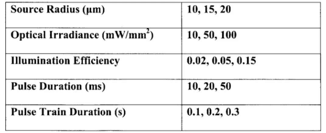
A parameter sweep was conducted, varying the source optical irradiance, the illumination efficiency, the pulse duration, total pulse train duration, and the source diameter. For this model, instead of the heat flux being varied, the optical irradiance is varied for several different illumination efficiencies (what percent of supplied power is converted to optical power). A summary of the parameters tested are shown in Table 1.

Table I - The different parameters used for the parameter sweep being described.

For all simulations, the stimulation frequency was held at 10 Hz. A series of summary plots

showing various relationships between parameters follows. The variable, eta, refers to

Source Radius (sm) 10, 15, 20

Optical Irradiance (mW/mm 2_{) 10, 50, 100}

Illumination Efficiency 0.02, 0.05, 0.15

Pulse Duration (ms) 10, 20, 50

illumination efficiency (ratio of electrical power delivered to source which gets converted to optical power). Obviously, all parameter combinations are not plotted.

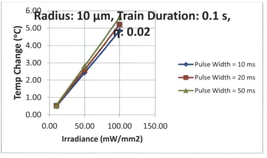
0.00 50.00 100.00 Irradiance (mW/mm2)

n: 0.1

s,

Figure 20 -Temperature change as a function of irradiance for several illumination efficiencies. As would be expected, as the illumination efficiency decreases, the temperature change increases (for any

given irradiance).

"Ra

E

-riU--

dius:

1'

/

[rain Nration: 0.1 s,

-t

U02

-U- Pulse Width = 20 ms

-*-Pulse Width = 50 ms

0.00 50.00 100.00 150.00

Irradiance (mW/mm2)

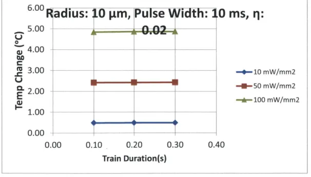
Figure 21 -Temperature change as a function of irradiance for several pulse widths. Although not a 0

to C

E

6.1 5.00 0 4.00 M 3.00 a 2.00

E

'idth:

10

ms,

rj:

-Train Duration = 0.1 sec

-U-Train Duration = 0.2 sec

--*-Train Duration = 0.3 sec

50.00 100.00 150.00

Irradiance (mW/mm2)

Figure 22 -Temperature change as a function of irradiance for several train durations. There is no significant change in temperature change as the total train duration is changed.

9_{0b Jration:}

_{.1 sec, P}

_ise

_{Wi h:}

₁₀

_ms,

_1:

8.00 7.00 6.00 C5.00 0 -+-Radius = 10 micron -- Radius = 15 micron E 3.00 -r- Radius = 20 micron - 2.00 -0.00 50.00 100.00 150.00 Irradiance (mW/mm2)

Figure 23 -Temperature change as a function of irradiance for several source sizes. As the radius decreases, the temperature change decreases (for any given irradiance). There are competing trends with this scaling: a smaller shank provides less heat conduction, but a smaller LED provides less heat

i dius: 10

-r-0.00

am,

_{Trair Jluratior}

F--20.00 -40.00

: 0.1 s, ri:

-E

Figure 24 -Temperature change as a function of pulse width for several irradiance values. Consistent with the results shown in Figure 21, the effect pulse width has on temperature change (for any given irradiance plot) is not significant, although noticeable. As the pulse widths are decreased further, the

different trends must converse at 0. 6.00 5 00 0 4.00 M 3.00 0-2.00 E, 1.UU 0.00 +-0.00

adius: .O

Vtm, IPulse Width: 40

ins, 11:

0.10 0.20 0.30 -+-10 mW/mm2 -0-50 mW/mm2 -r-100 mW/mm2 0.40 Train Duration(s)

Figure 25 -Temperature change as a function of total train duration for several irradiance values. Consistent with Figure 22, there is no detectable temperature change for different train durations (for any given irradiance trend). Obviously, as with the pulse duration, as the train duration approaches 0,

the temperature change must also converge to 0. However, at scales considered above, there is no

-+-10 mW/mm2 -1-50 mW/mm2 -,-100 mW/mm2

1.uu

u

lse

Wipth:

IF

ms,

-l

rain D

)2

uratio

n: 0.1 s

rl:

Figure 26 -Temperature change as a function of source radius for several irradiance values. Consistent with Figure 23, as the radius increases (for a given irradiance), the temperature change increases.

As stated before, the temperature change presented in Figures 20-26 are spatially located directly next to the LED in tissue. As can be seen in figures 18 and 19, the temperature changes over time in response to the stimulation pulse train. The temperature changes presented for figures 20-26 are the maximum over this stimulation time, and therefore represent the maximum temperature the tissue reaches. This model is for a single LED source in tissue. If there were multiple adjacent sources, the heating effect would be additive, and heating effects would be even more prevalent.

It should be noted that the temperature rises here presented are larger than the temperature rises presented in recent published work (McAlinden et al., 2013). The most likely reason for this is that the model matches the shank diameter with the LED diameter,

O% Co t( E.

E

I