Arboreal representations, sectional monodromy
groups, and abelian varieties over finite fields
by
Borys Kadets
Submitted to the Department of Mathematics
in partial fulfillment of the requirements for the degree of
Doctor of Philosophy
at the
MASSACHUSETTS INSTITUTE OF TECHNOLOGY
June 2020
c
○ Massachusetts Institute of Technology 2020. All rights reserved.
Author . . . .
Department of Mathematics
March 31, 2020
Certified by . . . .
Bjorn Poonen
Distinguished Professor in Science
Thesis Supervisor
Accepted by . . . .
Davesh Maulik
Graduate Co-Chair, Department of Mathematics
Arboreal representations, sectional monodromy groups, and
abelian varieties over finite fields
by
Borys Kadets
Submitted to the Department of Mathematics on March 31, 2020, in partial fulfillment of the
requirements for the degree of Doctor of Philosophy
Abstract
This thesis consists of three independent parts. The first part studies arboreal rep-resentations of Galois groups – an arithmetic dynamics analogue of Tate modules – and proves some large image results, in particular confirming a conjecture of Odoni. Given a field 𝐾, a separable polynomial 𝑓 ∈ 𝐾[𝑥], and an element 𝑡 ∈ 𝐾, the full backward orbit 𝒪−(𝑡) := ⋃︀
𝑘𝑓
∘−𝑘(𝑡) has a natural action of the Galois group Gal 𝐾.
For a fixed 𝑓 ∈ 𝐾[𝑥] with deg 𝑓 = 𝑑 and for most choices of 𝑡, the orbit 𝒪−(𝑡) has the structure of complete rooted 𝑑-ary tree 𝑇∞. The Galois action on 𝒪−(𝑡) thus
defines a homomorphism 𝜑 = 𝜑𝑓,𝑡 : Gal𝐾 → Aut 𝑇∞. The map 𝜑𝑓,𝑡 is the arboreal
representation attached to 𝑓 and 𝑡. In analogy with Serre’s open image theorem, one expects im 𝜑 = Aut 𝑇∞ to hold for most 𝑓, 𝑡, but until very recently for most degrees
𝑑 not a single example of a degree 𝑑 polynomial 𝑓 ∈ Q[𝑥] with surjective 𝜑𝑓,𝑡 was
known. Among other results, we construct such examples in all sufficiently large even degrees.
The second part concerns monodromy of hyperplane section of curves. Given a geometrically integral proper curve 𝑋 ⊂ P𝑛
𝐾, consider the generic hyperplane 𝐻 ∈
P
⋀︀
𝑛
𝐾(𝑡1,...,𝑡𝑛). The intersection 𝐻 ∩ 𝑋 is the spectrum of a finite separable field extension
𝐿/𝐾(𝑡1, ..., 𝑡𝑛) of degree 𝑑 := deg 𝑋. The Galois group 𝐺𝑋 := Gal(𝐿/𝐾(𝑡1, ..., 𝑡𝑛))
is known as the sectional monodromy group of 𝑋. When char 𝐾 = 0, the group 𝐺𝑋 equals 𝑆𝑑 for all curves 𝑋. This result has numerous applications in algebraic
geometry, in particular to the degree-genus problem. However, when char 𝐾 > 0, the sectional monodromy groups can be smaller. We classify all nonstrange nondegenerate curves 𝑋 ⊂ P𝑛, for 𝑛 > 3 such that 𝐺𝑋 ̸= 𝐴𝑑, 𝑆𝑑. Using similar methods we also
completely classify Galois group of generic trinomials, a problem studied previously by Abhyankar, Cohen, Smith, and Uchida.
In part three of the thesis we derive bounds for the number of F𝑞-points on simple
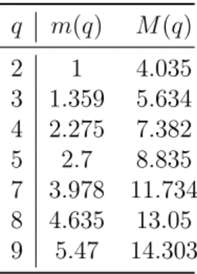
abelian varieties over finite fields; these improve upon the Weil bounds. For example, when 𝑞 = 3, 4 the Weil bound gives #𝐴(F𝑞) > 1 for all abelian varieties 𝐴. We prove
that 𝐴(F3) > 1.359dim 𝐴, and 𝐴(F4) > 2.275dim 𝐴 hold for all but finitely many simple
abelian varieties 𝐴 (with an explicit list of exceptions).
Thesis Supervisor: Bjorn Poonen
Acknowledgments
First and foremost I want to thank my advisor Bjorn Poonen for teaching me how to be a mathematician. I thank my fellow graduate students, and especially Bjorn’s army: Padma Srinivasan, Renee Bell, Isabel Vogt, Nicholas Triantafillou, Vishal Arul and Atticus Christensen for all their help and support. I thank my family for encouraging me to do mathematics professionally. I thank Davesh Maulik and Andrew Sutherland for serving on my thesis committee.
This research was supported by Simons Foundation grants #402472 (to Bjorn Poonen) and #550033, and National Science Foundation grant DMS-1601946.
Contents
1 A primer on Galois and monodromy groups 13
1.1 Étale fundamental groups . . . 14
1.2 Permutation groups . . . 17
1.3 Discretely valued fields and Newton polygons . . . 21
2 Arboreal Galois representations 25 2.1 Introduction . . . 25
2.2 Large arboreal representations over an arbitrary field . . . 28
2.3 Iterated monodromy groups . . . 35
2.4 Surjective arboreal representations over Q . . . . 36
3 Sectional monodromy groups 43 3.1 Introduction . . . 43
3.2 Transitivity of Sectional Monodromy Groups . . . 46
3.3 Tangents and inertia groups . . . 50
3.4 Sectional monodromy groups of nonstrange curves . . . 55
3.5 Galois groups of trinomials . . . 63
4.1 Introduction . . . 79 4.2 Abelian varieties over large fields . . . 82 4.3 Abelian varieties over small fields . . . 86
A Tables 91
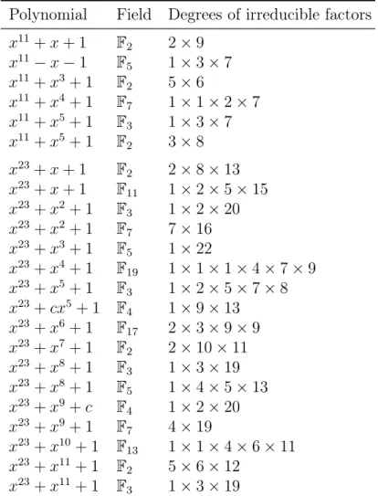
A.1 Cycle types of Mathieu groups . . . 91 A.2 Factors of trinomials over finite fields . . . 92
List of Figures
3-1 . . . 74 3-2 . . . 74
List of Tables
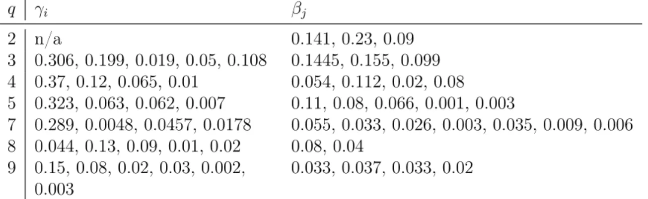
4.1 Lower and upper bounds on 𝑎(𝑞) and 𝐴(𝑞), respectively. . . 82
4.2 Lower and upper bounds on #𝐴(F𝑞)1/𝑔 . . . 87
4.3 Auxiliary polynomials for Theorem 4.3.2. . . 88
4.4 Auxiliary parameters for Theorem 4.3.2 . . . 89
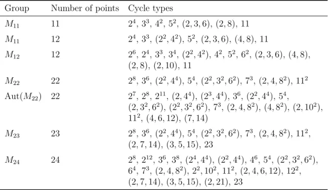
A.1 Cycle types of Mathieu groups . . . 91
Chapter 1
A primer on Galois and monodromy
groups
A finite degree 𝑑 topological covering of manifolds 𝑓 : 𝑌 → 𝑋 gives rise to a homo-morphism 𝜑 : 𝜋1(𝑋, 𝑥) → Aut(𝑓−1(𝑥)) = 𝑆𝑑 for any choice of basepoint1 𝑥 ∈ 𝑋. In
this way, the finite covering 𝑓 produces the group Mon(𝑓 ) := im 𝜑, the monodromy group of the covering. This construction is superficially similar to the formation of the Galois group of a finite separable field extension. The notion of the étale fun-damental group unifies geometric monodromy groups and arithmetic Galois groups and allows us to define monodromy groups attached to finite separable coverings of algebraic varieties.
This chapter introduces background and tools for determining algebraic mon-odromy groups. Section 1.1 contains a brief introduction to the theory of étale fun-damental groups. Section 1.2 collects various group-theoretic statements useful for computing monodromy groups. Section 1.3 collects basic facts about Galois groups of extensions of nonarchimedean local fields that are useful for studying local mon-odromy groups.
1Topological spaces often have basepoints, while schemes are more commonly equipped with base
1.1
Étale fundamental groups
Étale fundamental groups are an algebraic geometry analogue of fundamental groups in topology. Like fundamental groups, étale fundamental groups naturally act on fibers of finite “unramified” coverings of schemes. The correct algebraic version of the topological notion of unramified map is the following.
Definition 1.1.1. A morphism of schemes 𝜙 : 𝑌 → 𝑋 is called étale if it is smooth of relative dimension 0.
In other words, locally on 𝑌 the morphism 𝜙 corresponds to an extension of rings 𝐴 → 𝐵 of the form 𝐵 = 𝐴[𝑥1, . . . , 𝑥𝑛]/(𝑓1, . . . , 𝑓𝑛) such that the Jacobian determinant
det(𝜕𝑓𝑖/𝜕𝑥𝑗) is invertible in 𝐵. A morphism of C-varieties 𝑋 → 𝑌 is étale if and
only if it is biholomorphic.
Example 1.1.2. The following are examples of étale morphisms.
1. An open immersion 𝑌 → 𝑋.
2. A finite separable extension of fields Spec 𝐿 → Spec 𝐾.
3. The Artin-Schreier cover 𝜙 : A1𝐾 → A1𝐾 given by 𝜙(𝑥) = 𝑥𝑝 − 𝑥, where 𝑝 =
char 𝐾 > 0.
Suppose 𝑋 is a connected scheme. Fix a geometric point 𝑥 of 𝑋, that is a mor-phism 𝑥 : Spec𝐾 → 𝑋 for some algebraically closed field 𝐾. Let FÉt𝑋 denote the
category of finite étale coverings of 𝑋. Let 𝐹𝑥: FÉt𝑋 → Sets denote the functor
sending a covering 𝜙 : 𝑌 → 𝑋 to the fiber 𝜙−1(𝑥).
Fact 1.1.3 ([1] Section V.7). The category FÉt𝑋 is a Galois category and 𝐹𝑥 is
its fiber functor, so 𝐹𝑥 defines an equivalence of categories between FÉt𝑋 and the
category of Aut(𝐹𝑥)-sets.
In other words, there is a Galois correspondence between finite étale coverings of 𝑋 and open subgroups of the profinite group Aut(𝐹𝑥).
The group 𝜋et1 (𝑋, 𝑥) := Aut(𝐹𝑥) is called the étale fundamental group of 𝑋 with
base point 𝑥. The following theorem supports the claim that étale fundmental groups are similar to fundamental groups in topology. Recall that for a C-variety 𝑋 the set 𝑋(C) inherits the natural analytic topology from C.
Theorem 1.1.4 (“Riemann’s existence theorem”, [1] Theorem XII.5.1). Suppose 𝑋 is a connected separated scheme of finite type over C and 𝑥 ∈ 𝑋(C) is a point. There is a canonical isomorphism 𝜋1et(𝑋, 𝑥)→∼ ̂︀𝜋1(𝑋(C)top, 𝑥) between the étale fundamental
group of 𝑋, and the profinite completion of the topological fundamental group of 𝑋(C).
Remark 1.1.5. The hard part of Theorem 1.1.4 is to construct a canonical algebraic structure on a finite topological covering of 𝑋(C). When 𝑋 is proper, this can be done using GAGA, but for the general case more care is needed.
For varieties over fields that are not algebraically closed the structure of the étale fundamental group is more complicated. The simplest case is that of a point Spec 𝐾. Finite étale coverings of Spec 𝐾 are of the form Spec 𝐿 for 𝐿 =∏︀𝑛
𝑖=1𝐿𝑖a finite product
of finite separable field extensions 𝐿𝑖/𝐾. So the fundamental group of Spec 𝐾 is just
the absolute Galois group of 𝐾, 𝜋1et(Spec 𝐾) = Gal(𝐾sep/𝐾). For a general variety, the étale fundamental group is an extension of the Galois group of the ground field by the geometric fundamental group.
Theorem 1.1.6 ([1] Theorem V.6.1). Suppose 𝑋/𝐾 is a connected separated geo-metrically irreducible scheme of finite type and 𝑥 ∈ 𝑋(𝐾) a geometric point. Then there is a canonical exact sequence
1 → 𝜋1et(𝑋𝐾, 𝑥) → 𝜋1et(𝑋, 𝑥) → Aut(𝐾/𝐾) → 1.
Remark 1.1.7. If char 𝐾 = 0 and 𝑋 is normal, the group 𝜋et
1 (𝑋𝐾, 𝑥) is isomorphic to
𝜋1et(𝑋C, 𝑥).
Remark 1.1.8. If 𝐾 is an algebraically closed field of positive characteristic, and 𝑋/𝐾 a variety, then the structure of 𝜋1et(𝑋, 𝑥) can be much wilder than what one might
expect from the topological intuition. For example, the group 𝜋et1(A1
𝐾, 𝑥) is trivial
when char 𝐾 = 0, but not even finitely generated when char 𝐾 > 0.
Given a finite étale covering 𝑓 : 𝑌 → 𝑋 of degree 𝑑, we get a map 𝜑 : 𝜋et1 (𝑋, 𝑥) → Aut(𝐹𝑥(𝑌 )) = 𝑆𝑑. The image Mon(𝑓 ) := im 𝜑 ⊂ 𝑆𝑑 is called themonodromy group of
the covering 𝑓 ; it is a permutation group of degree 𝑑: a finite group with a specified action on a set of size 𝑑. Given two base points 𝑥, 𝑥′ ∈ 𝑋, there is a bijection 𝜓 : 𝐹𝑥(𝑌 ) → 𝐹𝑥′(𝑌 ) and an isomorphism 𝜋1(𝑋, 𝑥) → 𝜋1(𝑋, 𝑥′) making the following
diagram commute. 𝜋1(𝑋, 𝑥) −−−→ Aut(𝐹𝑥(𝑌 )) ⎮ ⎮ ⌄ ⎮ ⎮ ⌄𝜓 𝜋1(𝑋, 𝑥′) −−−→ Aut(𝐹𝑥′(𝑌 ))
In this way the monodromy group of the covering is independent of the choice of the base point. We will use the following properties of monodromy groups.
Proposition 1.1.9. Suppose that 𝑋 is a normal, connected, separated scheme and 𝑓 : 𝑌 → 𝑋 is a finite étale covering. Suppose 𝑈 ⊂ 𝑋 is an open subset and 𝜓 : 𝑋′ → 𝑋 a morphism.
1. The monodromy group Mon(𝑓 ) is transitive if and only if 𝑌 is irreducible. 2. The monodromy group Mon(𝑓 ) is imprimitive if and only if 𝑓 factorizes as a
composition of étale covers 𝑌 → 𝑌1 → 𝑋 of degrees strictly greater than 1
(primitivity is defined in Section 1.2).
3. ([1] Proposition V.8.2). Suppose 𝑈 ⊂ 𝑋 is an open subscheme. The monodromy group of the restricted covering 𝑓𝑈: 𝑌𝑈 → 𝑈 is equal to Mon(𝑓 ).
4. Suppose 𝑋′ is a connected scheme and 𝜓 : 𝑋′ → 𝑋 is a morphism. The mon-odromy group of the pullback 𝑋′ ×
𝑋 𝑌 → 𝑋
′ of 𝑓 under 𝜓 is a permutation
subgroup of Mon(𝑓 ).
5. ([1] Proposition V.8.2). If 𝑋, 𝑌 are of finite type over a field 𝐾, and 𝑓 is a 𝐾-morphism, then Mon(𝑓 ) is equal to the Galois group of the extension of function fields 𝐾(𝑌 )/𝐾(𝑋).
Remark 1.1.10. Normality of 𝑋 is an important assumption. For example, a nodal cubic over C admits cyclic étale covers 𝑌𝑛 → 𝑋 with 𝑌𝑛 isomorphic to a cyclic chain
of projective lines. Then property 1 does not hold, since the total space 𝑌𝑛 of the
cover is not irreducible. Property 5 is false, since the Galois group of C(𝑌𝑛) = C(𝑡)𝑛
over C(𝑡) is trivial, as is the monodromy of the covering restricted to the complement of the node, contradicting property 3. See [22] Exercise 10.6.
Monodromy groups are often calculated by combining the information on transi-tivity of 𝑌 → 𝑋 and related covers (for example, 𝑌 ×
𝑋𝑌 → 𝑋) with a computation of
monodromy of various pullbacks. Suppose 𝑋 is a variety over a field 𝐾, 𝑓 : 𝑌 → 𝑋 is a generically étale cover, and 𝑥 ∈ 𝑋 is a point over which 𝑓 is not étale. The monodromy of the pullback of 𝑌 → 𝑋 to the fraction field of the completed local ring Frac ˆ𝒪𝑋,𝑥 will be referred to as thelocal monodromy group of 𝑓 at 𝑥. These local
monodromy groups can often be described using the theory of local fields discussed in Section 1.3.
1.2
Permutation groups
We record here a selection of theorems on permutation groups that are useful for computing Galois groups.
Definition 1.2.1. Afinite permutation group is a triple (𝐺, 𝜑, 𝑆), where 𝐺 is a finite group, 𝑆 is a finite set, and 𝜑 : 𝐺 → Aut(𝑆) is an injective homomorphism. The size of 𝑆 is called the degree of 𝐺.
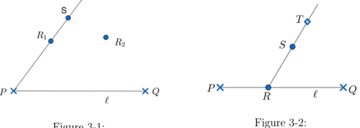
We will often abuse notation by referring to “a permutation group 𝐺” whenever the pair (𝜑, 𝑆) is clear from the context. A permutation group is𝑘-transitiveif 𝑘 6 #𝑆 and the group acts transitively on the 𝑘-tuples of distinct elements of 𝑆. A permutation group is primitive if it preserves no nontrivial partition of 𝑆. For example. the group of symmetries of the rooted tree below acting on the 6 vertices at the lower level is not primitive.
Example 1.2.2. Here is a list of some common permutation groups.
1. 𝐴𝑛, the alternating group on 𝑛 letters, it is an (𝑛 − 2)-transitive group.
2. AGL𝑛(𝑞), the affine general linear group, where 𝑛 > 1 and 𝑞 is a prime power.
It is a group of affine maps ⃗𝑥 → 𝐴⃗𝑥 + ⃗𝑏, where 𝐴 ∈ GL𝑛(𝑞), and ⃗𝑏 ∈ F𝑛𝑞. It
acts on A𝑛(F𝑞). It is a primitve and doubly transitive group. Since elements of
AGL𝑛(𝑞) preserve collinearity, the group is 3-transitive if and only if 𝑞 = 2.
3. AΓL𝑛(𝑞), the affine semilinear group. It is a permutation group acting on F𝑛𝑞
generated by AGL𝑛(𝑞) and the coordinate-wise 𝑝-power Frobenius.
4. PGL𝑛(𝑞), the projective general linear group, the group of linear symmetries of
the projective space P𝑛−1F𝑞 . It is a 2-transitive group. Since the group preserves
collinearity, it is 3-transitive if and only if 𝑛 = 2. The only 4-transitive group in the family is PGL2(3) = 𝑆4.
5. 𝑀11, the Mathieu group on 11 letters. It is defined as a one-point stabilizer of
the larger Mathieu group 𝑀12, which itself is the group of symmetries of the
unique 𝑆(5, 6, 12) Steiner system. The group 𝑀11 is a 4-transitive group. See
[15] for the construction of this sporadic simple group.
Many nontrivial results about permutation groups can be obtained as conse-quences of the classification of finite simple groups. We now outline some argu-ments that demonstrate the relationship between permutation groups and finite sim-ple groups.
Primitive groups can be naturally categorized into several classes. Suppose 𝐺 is primitive, and consider a minimal normal subgroup {1} ̸= 𝑁 ⊂ 𝐺. The orbits of 𝑁 on 𝑆 form a 𝐺-invariant partition of 𝑆. Since 𝐺 is primitive, 𝑁 has only one orbit, and so 𝑁 is transitive. Consider the centralizer 𝐶𝐺(𝑁 ); it is a normal subgroup
of 𝐺. Any two minimal normal subgroups 𝑁1, 𝑁2 of 𝐺 centralize each other, since
[𝑁1, 𝑁2] is a normal subgroup of 𝑁1 ∩ 𝑁2. If 𝐶𝐺(𝑁 ) = {1}, then 𝑁 is the unique
minimal normal subgroup and the conjugation action homomorphism 𝐺 → Aut 𝑁 is an injection. In this case 𝑁 is characteristically simple (see [50] Exercise 1.5.23), and so 𝑁 = 𝑇𝑛 for some simple group 𝑇 . Suppose 𝐶𝐺(𝑁 ) ̸= {1}; since 𝐶𝐺(𝑁 ) is a
nontrivial normal subgroup it acts transitively on 𝑆. If an element 𝑛 ̸= 1 of 𝑁 has a fixed point 𝑠 ∈ 𝑆, then 𝑛 also fixes every point of 𝐶𝐺(𝑁 )𝑠 = 𝑆, a contradiction.
Thus Stab(𝑠) ∩ 𝑁 = {1} and the action of 𝑁 on 𝑆 is regular (i.e. isomorphic to the action of 𝑁 on itself). This reasoning did not use minimiality of 𝑁 , so it applies also to the normal subgroup 𝐶𝐺(𝑁 ), Thus the action of 𝐶𝐺(𝑁 ) on 𝑆 is regular. Since
𝐶𝐺(𝑁 ) acts by automorphisms of the 𝑁 -torsor 𝑆, the group 𝐶𝐺(𝑁 ) is isomorphic to
𝑁 . If 𝑁 = 𝐶𝐺(𝑁 ), then 𝑁 is elementary abelian 𝑁 = F𝑛𝑝 since it is characteristically
simple, 𝑁 = 𝐶𝐺(𝑁 ), and the conjugation action of 𝐺 on 𝑁 defines an injection
𝐺/𝑁 → Aut(𝑁 ) = GL𝑁(F𝑝). Finally, suppose 𝑁 ̸= 𝐶𝐺(𝑁 ) and 𝐶𝐺(𝑁 ) ̸= 1. If
𝑁′ ̸= 𝑁 is a minimal normal subgroup of 𝐺, then 𝑁′ ⊂ 𝐶
𝐺(𝑁 ) and the action of 𝑁′
on 𝑆 is regular, so #𝑁′ = #𝑆 = #𝐶𝐺(𝑁 ) and 𝑁′ = 𝐶𝐺(𝑁 ). Hence 𝐺 has exactly two
minimal normal subgroups, and the socle of 𝐺 – the product of its minimal normal subgroups – is a power of a finite simple group.
The arguments outlined above can be developed much further, giving a complete classification of primitive permutation groups in terms of finite simple groups; the re-sulting statement is the O’Nan–Scott Theorem; see [16] Theorem 4.1A. Classification of finite simple groups combined with the O’Nan–Scott theorem gives very powerful tools for computing Galois and monodromy groups.
Given a finite étale covering 𝑓 : 𝑌 → 𝑋, the transitivity degree of the monodromy group can be read off the description of irreducible components of the fiber products
𝑌 ×𝑋 𝑌 ×𝑋 · · · ×𝑋 𝑌 . There are very few groups of high transitivity degree:
Theorem 1.2.3. [[13] Sections 7.3, 7.4] If 𝐺 is a triply transitive permutation group of degree 𝑑, then either 𝐺 ⊃ 𝐴𝑑 or one of the following holds:
1. 𝐺 = AGL𝑛(2), 𝑑 = 2𝑛;
2. 𝐺 = 𝐺1, 𝑑 = 16 (a special permutation subgroup of AGL4(2));
3. PSL2(𝑟) ⊂ 𝐺 ⊂ PΓL2(𝑟), 𝑑 = 𝑟 + 1, 𝑟 is a power of a prime;
4. 𝐺 = 𝑀11, 𝑑 = 11 (a Mathieu group, see [15]);
5. 𝐺 = 𝑀11, 𝑑 = 12; 6. 𝐺 = 𝑀12, 𝑑 = 12 7. 𝐺 = 𝑀22, 𝑑 = 22; 8. 𝐺 = Aut(𝑀22), 𝑑 = 22; 9. 𝐺 = 𝑀23, 𝑑 = 23; 10. 𝐺 = 𝑀24, 𝑑 = 24.
Remark 1.2.4. The classification of 2-transitive groups is also known, see [16] Sec-tion 7.7.
Another common input to the computation of a monodromy group is a local cal-culation. Local monodromy groups often contain cycles. Primitive groups containing cycles can be classified:
Theorem 1.2.5 (Jones [25]). Let 𝐺 be a primitive permutation group of finite degree 𝑑, not containing 𝐴𝑑. Suppose that 𝐺 contains a cycle fixing exactly 𝑘 points, where
0 6 𝑘 6 𝑑 − 2. Then one of the following holds:
1. 𝑘 = 0 and either
(b) PGL𝑛(𝑞) ⊂ 𝐺 ⊂ PΓL𝑛(𝑞) with 𝑑 = (𝑞𝑛− 1)/(𝑞 − 1) and 𝑛 > 2 for some
prime power 𝑞, or
(c) 𝐺 = PSL2(11), 𝑀11 or 𝑀23 with 𝑑 = 11, 11, 23, respectively.
2. 𝑘 = 1 and either
(a) AGL𝑛(𝑞) ⊂ 𝐺 ⊂ AΓL𝑛(𝑞) with 𝑑 = 𝑞𝑛 and 𝑛> 1 for some prime power 𝑞,
or
(b) 𝐺 = PSL2(𝑝) or 𝐺 = PGL2(𝑝) with 𝑑 = 𝑝 + 1 for some prime 𝑝 > 5, or
(c) 𝐺 = 𝑀11, 𝑀12 or 𝑀24 with 𝑑 = 12, 12, 24, respectively.
3. 𝑘 = 2 and PGL2(𝑞) ⊂ 𝐺 ⊂ PΓL2(𝑞) with 𝑑 = 𝑞 + 1 for some prime power 𝑞.
Even when local monodromy does not have cycles, but has sufficiently many fixed points, one can still conclude that the monodromy group is large. Theminimal degree
𝜇(𝐺) of a permutation group 𝐺 is the minimum over 𝑔 ∈ 𝐺 ∖ {1} of the number of points not fixed by 𝑔.
Theorem 1.2.6 (Liebeck-Saxl [37] Corollary 3). Let 𝐺 be a primitive permutation group of degree 𝑑, and assume that 𝐺 ̸⊃ 𝐴𝑑. Then 𝜇(𝐺) > 2(
√
𝑑 − 1). Remark 1.2.7. There is a classification of groups with 𝜇(𝐺) < 𝑑/2, see [19].
1.3
Discretely valued fields and Newton polygons
We briefly summarize the basics of the theory of local fields and their extensions, a detailed treatment can be found in [48].
Definition 1.3.1. A complete discretely valued field is a pair (𝐹, 𝑣𝐹), where 𝐹 is a
field complete with respect to the discrete valuation 𝑣 = 𝑣𝐹: 𝐹 → Q (the image of
𝑣 is an infinite cyclic group). The ring 𝒪𝐹 = {𝑥 ∈ 𝐹 |𝑣(𝑥) > 0} ⊂ 𝐹 is called the
valuation ring of 𝐹 . An element 𝜋 ∈ 𝒪𝐹 is called a uniformizer if 𝑣(𝜋) is a generator
Example 1.3.2.
1. 𝐹 = Q𝑝 with 𝑣 = 𝑣𝑝 the 𝑝-adic valuation. The element 𝜋 = 𝑝 is a uniformizer,
and F𝑝 = Z𝑝/(𝑝) is the residue field.
2. 𝐹 = 𝑘((𝑡)), and 𝑣 is the 𝑡-adic valuation. The element 𝑡 is a uniformizer and 𝑘 is the residue field.
3. 𝐹 = Q𝑝(
√
𝑝), the valuation 𝑣 is defined by 𝑣(𝑥) = 𝑣𝑝(︀Norm𝐹 /Q𝑝(𝑥))︀ /2. The
element √𝑝 is a uniformizer and F𝑝 is the residue field.
Given a finite extension 𝐿 of a complete discretely valued field 𝐹 , there is a unique extension of 𝑣 to a discrete valuation 𝑣𝐿on 𝐿, defined by 𝑣𝐿: 𝐿 → Q, 𝑣𝐿(𝑥) :=
𝑣𝐹(Norm𝐿/𝐹(𝑥))/[𝐿 : 𝐹 ]. The pair (𝐿, 𝑣𝐿) is a discretely valued field. Theramification
index 𝑒𝐿/𝐹 of 𝐿/𝐹 is the index 𝑒𝐿/𝐹 := [𝑣𝐿(𝐿) : 𝑣𝐹(𝐹 )] of the extension of value
groups. An extension 𝐿/𝐹 is totally ramified if 𝑒𝐿/𝐹 = [𝐿 : 𝐹 ], and is tamely ramified
if char 𝑘𝐹 - 𝑒𝐿/𝐹. The field 𝑘𝐹 = 𝒪𝐹/𝜋𝐹 = 𝒪𝐹/ (𝜋𝐿𝒪𝐿∩ 𝒪𝐹) is a subfield of 𝑘𝐿; thus
an extension of discretely valued fields 𝐿/𝐹 gives rise to an extension of residue fields 𝑘𝐿/𝑘𝐹. The degree 𝑓𝐿/𝐾 := [𝑘𝐿: 𝑘𝐹] is called theinertia degree of 𝐿/𝐾. An extension
𝐿/𝐹 is unramified if 𝑒𝐿/𝐹 = 1 and the residue field extension 𝑘𝐿/𝑘𝐹 is separable.
Proposition 1.3.3. Suppose 𝐹 is a discretely valued field with perfect residue field 𝑘𝐹.
1. Every separable extension 𝐿/𝐹 can be extended to a tower 𝐿/𝐿′/𝐹 , where 𝐿/𝐿′ is totally ramified and 𝐿′/𝐹 is unramified.
2. The functor sending a finite field extension 𝐿/𝐹 to the residue field extension 𝑘𝐿/𝑘𝐹 defines an equivalence of categories
{unramified field extensions of 𝐹 }→ {finite extensions of 𝑘∼ 𝐹}.
4. If 𝐹 = 𝑘((𝑡)), then any finite extension 𝐿/𝐹 is isomorphic to 𝑘𝐿((𝑢)).
5. If 𝐹 = 𝑘((𝑡)) and 𝑘 is algebraically closed, then any tamely ramified extension 𝐿/𝐹 is of the form 𝐿 = 𝑘((𝑡1/𝑒)) with char 𝐾 - 𝑒.
Newton polygons, defined below, are a versatile tool for determining valuations of roots of polynomials.
Definition 1.3.4. Suppose 𝐹 is a discretely valued field, and 𝑓 = 𝑎0+ · · · + 𝑎𝑛𝑥𝑛∈
𝐹 [𝑥] is a polynomial with 𝑎0 ̸= 0. Consider the set of points 𝑆 = {(𝑖, 𝑣(𝑎𝑖)) : 0 6
𝑖 6 𝑛} in R2. The Newton Polygon NP(𝑓 ) of 𝑓 is the lower convex hull of 𝑆. The
Newton polygon consists of segments of distinct slopes connecting vertices in 𝑆. A
width of a segment from (𝑥1, 𝑦1) to (𝑥2, 𝑦2) is defined to be 𝑥2− 𝑥1, and the slope of
this segment is 𝑦1−𝑦2
𝑥1−𝑥2.
Example 1.3.5. Consider the polynomial 𝑓 = 𝑝 + 𝑝𝑥 + 𝑥2+ 𝑝2𝑥3+ 𝑝2𝑥4 ∈ Q
𝑝[𝑥]. The
Newton polygon of 𝑓 consists of two segments connecting consecutive vertices (0, 1), (2, 0), and (4, 2). One segment has slope −1/2 and width 2, and the other segment has slope 1 and width 2.
The Newton polygon of 𝑓 determines valuations of the roots of 𝑓 .
Proposition 1.3.6 (see [34] Section IV.3). Suppose 𝐹 is a discretely valued field and 𝑓 ∈ 𝐹 [𝑥] is a polynomial with nonzero constant term. Extend the valuation 𝑣𝐹 on
𝐹 to a valuation 𝑣 : 𝐹 → Q. Consider the Newton polygon 𝑁𝑃 (𝑓 ) of 𝑓 . Then the number of zeros of 𝑓 with valuation 𝛼 is the width of the segment of slope −𝛼 (the width is 0 if such segment does not exist).
Example 1.3.7 (Eisenstein polynomials). Consider a polynomial 𝑎0+· · ·+𝑎𝑛−1𝑥𝑛−1+
𝑥𝑛∈ 𝐹 [𝑥] such that 𝑣(𝑎
0) = 1, 𝑣(𝑎𝑖) > 1 for 1 6 𝑖 6 𝑛 − 1. The Newton polygon of 𝑓
consists of one segment of width 𝑛 and slope −1/𝑛. Let 𝛼 ∈ 𝐹 be a root of 𝑓 . From the Newton polygon we conclude 𝑣(𝛼) = 1/𝑛. Therefore the extension 𝐹 (𝛼)/𝐹 has ramification index at least 𝑛. Since the degree deg 𝐹 (𝛼)/𝐹 is at most 𝑛 we conclude that 𝑓 is an irreducible polynomial and 𝐹 (𝛼)/𝐹 is a totally ramified extension of degree 𝑛.
Remark 1.3.8. In a similar fashion, Newton Polygons can be used to determine valu-ations of roots of convergent power series; see [34] Section IV.4.
Chapter 2
Arboreal Galois representations
The results of this chapter have appeared in [31].
2.1
Introduction
Let 𝐾 be a field, let 𝑓 ∈ 𝐾[𝑥] be a polynomial of degree 𝑑, and let 𝑡 ∈ 𝐾 be an arbitrary element. Write 𝑓∘𝑛 = 𝑓 ∘ 𝑓 ∘ · · · ∘ 𝑓 for the 𝑛th iterate of 𝑓 (with the convention 𝑓∘0(𝑥) = 𝑥). Assume that the polynomials 𝑓∘𝑛(𝑥) − 𝑡 are separable for all 𝑛 ≥ 0. Fix a separable closure 𝐾sep of 𝐾. Then the roots of 𝑓∘𝑛(𝑥) − 𝑡 in 𝐾sep
for varying 𝑛 have a natural tree structure. Namely, define a graph with the set of vertices equal to the disjoint union of roots of 𝑓∘𝑛(𝑥) − 𝑡 for all 𝑛 ≥ 0. Draw an edge between two roots 𝛼, 𝛽 when 𝑓 (𝛼) = 𝛽. Then when 𝑡 is not a periodic point of 𝑓 , the resulting graph is a complete rooted 𝑑-ary tree 𝑇∞. Vertices at level 𝑛 correspond
to the roots of 𝑓∘𝑛(𝑥) − 𝑡 (the root of the tree 𝑡 is at level zero). Let 𝑇𝑛 be the tree
formed by levels 0 through 𝑛 of 𝑇∞. For example, the next figure is the tree 𝑇2 when
0
−√2 √2
√︀
2 −√2 −√︀2 −√2 √︀2 +√2 −√︀2 +√2
Let 𝐺 := Gal(𝐾sep/𝐾) be the absolute Galois group of 𝐾. The Galois action on
𝐾sep defines a homomorphism 𝜑 : 𝐺 → Aut(𝑇∞) known as the arboreal Galois
repre-sentationattached to 𝑓 and 𝑡. This construction is parallel to that of the Tate module of an abelian variety, where one replaces 𝑓 by the multiplication by 𝑝 endomorphism [𝑝]. With this analogy in mind, it is natural to seek a counterpart of Serre’s open image theorem in arithmetic dynamics. The crucial difference is that while the closed subgroups of GL2(Z𝑝) are easy to describe using Lie theory, the subgroup structure of
the profinite group Aut(𝑇∞) is complicated; this makes analyzing possibilities for the
image of an arboreal representation a hard problem. Our goal is to study conditions for having the simplest kind of Galois image, namely the whole group Aut(𝑇∞).
Example 2.1.1. Let 𝐾 = Q, 𝑡 = 0 and 𝑓 = 𝑥2+ 1. Then the arboreal representation is surjective (see [54]).
It is conjectured that when 𝐾 is a number field and 𝑑 = 2, the image of an arboreal representation has finite index in Aut(𝑇∞) unless some degeneracy conditions are
satisfied (see [26, Conjecture 3.11]). However, very little is known when the degree of 𝑓 is greater than 2. We will show that when the degree of 𝑓 is even, there is a criterion for the surjectivity of the arboreal representation; this generalizes the method of Stoll in [54]. In Section 2.2 we prove the following theorem.
Theorem 2.1.2. Assume that the degree of 𝑓 is even and char 𝐾 ̸= 2. Assume that for any 𝑛 and any 𝛼 ∈ 𝑓−𝑛(𝑡) the splitting field of 𝑓 (𝑥) − 𝛼 over 𝐾(𝛼) has Galois group 𝑆𝑑. If the discriminants disc(𝑓∘𝑛(𝑥) − 𝑡) are linearly independent in
the F2-vector space 𝐾×/𝐾×2, then the arboreal representation attached to 𝑓 and 𝑡 is
This theorem allows us to prove surjectivity of some arboreal representations at-tached to even degree polynomials. The following conjecture was made by Odoni in [45, Conjecture 7.5.]
Conjecture 2.1.3. Let 𝐹 be a Hilbertian field. Then for any integer 𝑑 there exists a degree 𝑑 monic polynomial 𝑓 such that the associated arboreal representation (for 𝑡 = 0) is surjective.
Until recently, the conjecture was open even for 𝐹 = Q (see [26, Conjecture 2.2]). Looper [38] proved Odoni’s conjecture for 𝐹 = Q and prime degrees 𝑑, and showed that for many other values of 𝑑 Odoni’s conjecture can be deduced from Vojta’s conjecture. In Section 2.4 we prove the following theorem unconditionally.
Theorem 2.1.4. Let 𝑑 ≥ 20 be an even number. Then there exist infinitely many polynomials 𝑓 ∈ Q[𝑥] of degree 𝑑 such that the arboreal representation associated to 𝑓 and 𝑡 = 0 is surjective.
Independently of our work, Joel Specter [53] and Robert Benedetto and Jamie Juul [10] proved related results on Odoni’s conjecture for number fields. Specter shows that Odoni’s conjecture holds for any number field. Benedetto and Juul prove Odoni’s conjecture for even degree polynomials over an arbitrary number field, and for odd degree 𝑑 polynomials over number fields 𝐹 that do not contain Q(√𝑑,√𝑑 + 1).
Consider the case when 𝐾 = 𝐹 (𝑢) for some field 𝐹 and indeterminate 𝑢, 𝑓 is a polynomial defined over 𝐹 , and 𝑡 = 𝑢. Let 𝐾𝑛 be the splitting field of 𝑓∘𝑛(𝑥) − 𝑡
over 𝐾. Then the groups Gal(𝐾𝑛/𝐾) are the monodromy groups of the ramified
coverings P1
𝐹 → P1𝐹 induced by 𝑓
∘𝑛. In this case the image of the resulting arboreal
representation is known as the iterated monodromy group of 𝑓 . These monodromy groups have been studied in the case when 𝑓 is post-critically finite (see [44]), when 𝑓 is quadratic (see [46]), and for various rational functions 𝑓 in [28]. Recall that a polynomial 𝑓 is called post-critically finite if for every root 𝛾 of 𝑓′the orbit of 𝛾 under 𝑓 is finite. In Section 2.3 we prove the following theorem.
Theorem 2.1.5. Let 𝑓 ∈ 𝐹 [𝑥] be a degree 2𝑚 polynomial such that the Galois group of the splitting field of 𝑓 (𝑥) − 𝑡 over 𝐾 = 𝐹 (𝑡) is the symmetric group 𝑆2𝑚. Assume
that 𝑓′(𝑥) is irreducible over 𝐹 and 𝑓 is not post-critically finite. Then the arboreal representation attached to 𝑓 and 𝑡 over 𝐾 is surjective.
In fact we prove a stronger statement that provides a criterion for the surjectivity of the iterated monodromy group attached to an even degree polynomial 𝑓 in terms of the critical orbit of 𝑓 . Jamie Juul [28, Proposition 3.2.] proves a version of Theorem 2.1.5 for finite level arboreal representations and polynomials of arbitrary degree. However, we do not know if there are many polynomials for which Juul’s result implies surjectivity of the infinite level arboreal representation is large. Our result shows that when 𝐹 is a number field most polynomials have surjective infinite level iterated monodromy groups, see Remark 2.3.3.
2.2
Large arboreal representations over an arbitrary
field
We begin by introducing some arboreal notation. Fix a field 𝐾 of characteristic not 2, a polynomial 𝑓 ∈ 𝐾[𝑥] of degree 𝑑, and an element 𝑡 ∈ 𝐾. Assume 𝑡 is not periodic under 𝑓 , and assume that the polynomials 𝑓∘𝑛(𝑥) − 𝑡 are separable for all 𝑛. Write 𝑇∞ for the preimage tree of 𝑡 under 𝑓 as in the introduction. Let 𝐾𝑛/𝐾 denote the
splitting field of 𝑓∘𝑛(𝑥) − 𝑡 over 𝐾. Denote by 𝑇𝑛the tree formed by the first 𝑛 levels
of 𝑇∞. The Galois group Gal(𝐾𝑛/𝐾) injects into the automorphism group of the tree
Aut(𝑇𝑛). We call the extension 𝐾𝑛/𝐾 maximal if Gal(𝐾𝑛/𝐾) = Aut(𝑇𝑛).
The aim of this section is to prove a criterion for surjectivity of arboreal repre-sentations 𝜑 : 𝐺 → Aut(𝑇∞). We establish surjectivity in three steps. Step one is to
show that for all 𝑛 and 𝛼 ∈ 𝑓−𝑛(𝑡) the Galois group of the splitting field of 𝑓 (𝑥) − 𝛼 over 𝐾(𝛼) is 𝑆𝑛. Step two is to show that the splitting field of 𝑓 (𝑥)−𝛼 is disjoint from
fields of 𝑓 (𝑥) − 𝛼𝑖 for different 𝛼𝑖 ∈ 𝑓−𝑛(𝑡) are linearly disjoint. We show that steps
two and three can be reduced to the arithmetic of forward orbits of 𝑓 .
The main idea is simple: any proper normal subgroup of 𝑆𝑑 is contained in 𝐴𝑑;
therefore to show that some 𝑆𝑑 extensions are linearly disjoint it is enough to show
that their (unique) quadratic subfields are linearly disjoint, as we will now prove. Lemma 2.2.1. Let 𝐿/𝐾 be a Galois extension of fields with Galois group 𝑆𝑑. Let 𝐹
denote the unique quadratic extension of 𝐾 contained in 𝐿. Let 𝑀/𝐾 be an arbitrary Galois extension. Then the fields 𝐿 and 𝑀 are linearly disjoint over 𝐾 if and only if the fields 𝐹 and 𝑀 are linearly disjoint over 𝐾.
Proof. If 𝐿 and 𝑀 are disjoint, then so are 𝐹 and 𝑀 . Assume that 𝐹 and 𝑀 are disjoint. The field extension 𝐾 ⊂ (𝐿 ∩ 𝑀 ) ⊂ 𝐿 corresponds to a normal subgroup of 𝑆𝑑. Any nontrivial normal subgroup of 𝑆𝑑 is contained in 𝐴𝑑 and therefore if 𝐿 ∩ 𝑀
were not 𝐾 it would contain 𝐹 .
Lemma 2.2.2. Let 𝐿𝑖/𝐾 for 𝑖 = 1, . . . , 𝑛 be 𝑆𝑑-Galois extensions of 𝐾. Let 𝐹𝑖 ⊂ 𝐿𝑖
denote the unique quadratic extension of 𝐾 inside 𝐿𝑖. Then the fields 𝐿𝑖 are linearly
disjoint if and only if the fields 𝐹𝑖 are linearly disjoint.
Proof. If 𝐿𝑖 are linearly disjoint, then 𝐹𝑖 are also linearly disjoint. Assume that 𝐹𝑖 are
linearly disjoint. We use induction on 𝑛. The case 𝑛 = 2 follows from Lemma 2.2.1. Suppose that the result holds for 𝑛 − 1. Then the fields 𝐿1, . . . , 𝐿𝑛−1 are linearly
disjoint. Let 𝑀 denote the compositum 𝐿1. . . 𝐿𝑛−1. The Galois group Gal(𝑀/𝐾)
is isomorphic to (𝑆𝑑)𝑛−1. We need to show that 𝑀 and 𝐿𝑛 are disjoint. By Lemma
2.2.1 it is enough to show that 𝐹𝑛 and 𝑀 are disjoint.
Let 𝐹/𝐾 be a quadratic extension of 𝐾 contained in 𝑀 . Then 𝐹 defines a character 𝜒 : (𝑆𝑑)
𝑛−1
= Gal(𝑀/𝐾) → {±1}. The character 𝜒 can be written as
𝜒(𝑎1, . . . , 𝑎𝑛−1) = 𝜒1(𝑎1) · · · 𝜒𝑛−1(𝑎𝑛−1), (𝑎1, . . . , 𝑎𝑛−1) ∈ 𝑆𝑑× · · · × 𝑆𝑑,
characters: the trivial character and the sign character. Let 𝑏𝑖 ∈ 𝐾 be elements
such that 𝐹𝑖 = 𝐾(
√
𝑏𝑖). Let 𝐼 ⊂ {1, . . . , 𝑛 − 1} be the set of indices 𝑖 for which 𝜒𝑖
is nontrivial. Then the extension 𝐹 is obtained by adjoining to 𝐾 a square root of ∏︀
𝑖∈𝐼𝑏𝑖. In particular, since 𝐹𝑛 is disjoint from the compositum 𝐹1. . . 𝐹𝑛−1, it is not
a subfield of 𝑀 and therefore 𝑀 and 𝐿𝑛 are disjoint.
Lemma 2.2.2 allows us to reduce proving surjectivity of an arboreal representation to Kummer theory. We also need a standard fact about discriminants.
Lemma 2.2.3. Let 𝑆 be a commutative ring, let 𝑃, 𝑄 ∈ 𝑆[𝑥] be arbitrary polyno-mials. Then disc(𝑃 𝑄) = (−1)deg 𝑃 deg 𝑄disc(𝑃 ) disc(𝑄)𝑅(𝑃, 𝑄)2 where 𝑅(𝑃, 𝑄) is the
resultant of 𝑃 and 𝑄.
Proof. We recall the normalization of discriminant and resultant for non-monic poly-nomials from [35, Chapter IV §8]. Assume 𝑃, 𝑄 have degrees 𝑛, 𝑚, leading coef-ficients 𝑎, 𝑏, and roots 𝛼1, . . . , 𝛼𝑛 and 𝛽1, . . . , 𝛽𝑚. Then the resultant is given by
𝑅(𝑃, 𝑄) = 𝑎𝑚𝑏𝑛∏︀
𝑖,𝑗(𝛼𝑖−𝛽𝑗), and the relevant discriminants are given by the formulas
disc(𝑃 ) = (−1)𝑛(𝑛−1)/2𝑎2𝑛−2∏︀ 𝑖̸=𝑗(𝛼𝑖−𝛼𝑗), disc(𝑄) = (−1)𝑚(𝑚−1)/2𝑏2𝑛−2 ∏︀ 𝑖̸=𝑗(𝛽𝑖−𝛽𝑗), and disc(𝑃 𝑄) = (−1)(𝑛+𝑚)(𝑛+𝑚−1)/2(𝑎𝑏)2(𝑛+𝑚)−2∏︁ 𝑖̸=𝑗 (𝛼𝑖− 𝛼𝑗) ∏︁ 𝑖̸=𝑗 (𝛽𝑖− 𝛽𝑗) ∏︁ 𝑖,𝑗 (𝛼𝑖− 𝛽𝑗)2.
Fix a field 𝐾 of characteristic not 2 and fix an element 𝑡 ∈ 𝐾. Let 𝑓 ∈ 𝐾[𝑥] be a degree 𝑑 polynomial where 𝑑 is even. Consider the corresponding tree 𝑇∞, arboreal
representation 𝜑 : 𝐺 → Aut(𝑇∞), and the extensions 𝐾𝑛/𝐾.
Theorem 2.2.4. Assume that for some 𝑛 ∈ Z>0 the field extension 𝐾𝑛−1/𝐾 is
maximal. Assume also that for every 𝛼 ∈ 𝑓−(𝑛−1)(𝑡) the polynomial 𝑓 (𝑥) − 𝛼 is irreducible over 𝐾(𝛼) and has Galois group 𝑆𝑑 or 𝐴𝑑. Then 𝐾𝑛/𝐾 is maximal if and
Proof. Assume that 𝐾𝑛/𝐾 is maximal. Then the Galois group of 𝐾𝑛/𝐾𝑛−1 acts on
the roots of 𝑓∘𝑛(𝑥) − 𝑡 as a product of 𝑑𝑛−1 copies of 𝑆
𝑑. In particular there is an
element of Gal(𝐾𝑛/𝐾𝑛−1) that induces an odd permutation of the roots of 𝑓∘𝑛(𝑥) − 𝑡.
Therefore disc(𝑓∘𝑛(𝑥) − 𝑡) is not a square in 𝐾𝑛−1.
Now assume disc(𝑓∘𝑛(𝑥) − 𝑡) ̸∈ 𝐾𝑛−1×2 . For any choice of the root 𝛼 of 𝑓∘𝑛−1(𝑥) − 𝑡 consider the discriminant disc(𝑓 (𝑥) − 𝛼). Assume that disc(𝑓 (𝑥) − 𝛼) is a square in 𝐾𝑛−1. Since the extension 𝐾𝑛−1/𝐾 is maximal, the Galois action on the roots
𝛼𝑖 ∈ 𝑓−(𝑛−1)(𝑡) is transitive. Therefore for every 𝛼𝑖 the discriminant disc(𝑓 (𝑥) − 𝛼𝑖)
is in 𝐾𝑛−1×2 as well. By Lemma 2.2.3 the following identity holds
∏︁ 𝛼∈𝑓−(𝑛−1)(𝑡) disc (𝑓 (𝑥) − 𝛼) ≡ disc ⎛ ⎝ ∏︁ 𝛼∈𝑓−(𝑛−1)(𝑡) (𝑓 (𝑥) − 𝛼) ⎞ ⎠ ≡ disc(𝑓∘𝑛(𝑥) − 𝑡) ̸≡ 1 (mod 𝐾𝑛−1×2 ).
Therefore disc(𝑓 (𝑥) − 𝛼) ̸∈ 𝐾𝑛−1×2 and the Galois group of 𝑓 (𝑥) − 𝛼 over 𝐾(𝛼) is equal to 𝑆𝑑. By Lemma 2.2.1, applied to the splitting field of 𝑓 (𝑥) − 𝛼 over 𝐾(𝛼)
and 𝐾𝑛−1/𝐾(𝛼), the polynomial 𝑓 (𝑥) − 𝛼 is irreducible over 𝐾𝑛−1 and has the Galois
group equal to 𝑆𝑑. In order to apply Lemma 2.2.2 we need to show that disc(𝑓 (𝑥)−𝛼𝑖)
are linearly independent in the F2 vector space 𝐾𝑛−1× /𝐾 ×2 𝑛−1.
We claim that for 𝑚 ≤ 𝑛 − 1 and 𝛽𝑖 ∈ 𝑓−𝑚(𝑡) the elements disc(𝑓𝑛−𝑚(𝑥) − 𝛽𝑖)
are linearly independent in the F2 vector space 𝐾𝑛−1× /𝐾 ×2
𝑛−1. We prove the statement
by induction. When 𝑚 = 0 the statement holds by the assumption of the theorem. Assume the statement is true for 𝑚 = 𝑙 − 1. Assume that there is a nonempty subset 𝐽 ⊂ 𝑓−𝑙(𝑡) such that∏︀
𝛽∈𝐽disc(𝑓
∘𝑛−𝑙(𝑥) − 𝛽) is a square. Say that 𝛽
𝑖 and 𝛽𝑗 belong
to the same cluster if 𝑓 (𝛽𝑖) = 𝑓 (𝛽𝑗) (in other words 𝛽𝑖 and 𝛽𝑗 have the same parent in
with 𝐽 , then 𝑓−1(𝑓 (𝐽 )) = 𝐽 , and so by Lemma 2.2.3 ∏︁ 𝛽∈𝐽 disc(𝑓∘𝑛−𝑙(𝑥) − 𝛽) ≡ ∏︁ 𝛾∈𝑓 (𝐽 ) ∏︁ 𝛽∈𝑓−1(𝛾) disc(𝑓∘𝑛−𝑙(𝑥) − 𝛽) ≡ ∏︁ 𝛾∈𝑓 (𝐽 ) disc(𝑓𝑛−𝑙+1(𝑥) − 𝛾) (mod 𝐾𝑛−1×2 ).
The right hand side is not a square by the induction hypothesis. Therefore, we can assume that there is a cluster 𝐼 such that 𝐼 has a nontrivial intersection with 𝐽 . Choose two elements 𝛽′, 𝛽′′ ∈ 𝐼 such that 𝛽′ is in 𝐽 and 𝛽′′ is not in 𝐽 . Since the
extension 𝐾𝑛−1/𝐾 is assumed to be maximal, there exists an element 𝜎 ∈ Gal(𝐾𝑙/𝐾)
that acts on the roots of 𝑓∘𝑙(𝑥) − 𝑡 as a transposition of 𝛽′ and 𝛽′′. Then
1 ≡ (︃ ∏︁ 𝛽∈𝐽 disc(𝑓∘𝑛−𝑙(𝑥) − 𝛽) )︃ · 𝜎 (︃ ∏︁ 𝛽∈𝐽 disc(𝑓∘𝑛−𝑙(𝑥) − 𝛽) )︃
≡ disc(𝑓∘𝑛−𝑙(𝑥) − 𝛽′) disc(𝑓∘𝑛−𝑙(𝑥) − 𝛽′′) (mod 𝐾𝑛−1×2 ).
Since Gal(𝐾𝑙/𝐾) acts doubly-transitively on the cluster, for every pair of elements
𝛽𝑖, 𝛽𝑗 ∈ 𝐼 the product disc(𝑓∘𝑛−𝑙(𝑥)−𝛽𝑖) disc(𝑓∘𝑛−𝑙(𝑥)−𝛽𝑗) is a square in 𝐾𝑛−1. Since
𝑑 is even, the product ∏︀
𝛽∈𝐼disc(𝑓
∘𝑛−𝑙− 𝛽) is a square in 𝐾
𝑛−1. By Lemma 2.2.3 we
have the identity
∏︁
𝛽∈𝐼
disc(𝑓∘𝑛−𝑙(𝑥) − 𝛽) ≡ disc(𝑓𝑛−𝑙+1(𝑥) − 𝑓 (𝛽)) (mod 𝐾𝑛−1×2 ),
where the right hand side is not a square by the induction hypothesis. Therefore the elements disc(𝑓∘𝑛−𝑙− 𝛽𝑖) are linearly independent mod𝐾𝑛−1×2 .
Now we can apply Lemma 2.2.2 to the extensions given by the splitting fields of 𝑓 (𝑥) − 𝛼𝑖 over 𝐾𝑛−1. We have proved that each extension is an 𝑆𝑑 extension. The
unique quadratic subextension of this splitting field is 𝐾𝑛−1
(︁
√︀disc (𝑓(𝑥) − 𝛼𝑖)
)︁ . Since disc(𝑓 (𝑥) − 𝛼𝑖) are linearly independent in 𝐾𝑛−1/𝐾𝑛−1×2 , the corresponding
Proposition 2.2.5. Assume that the extension 𝐾𝑛/𝐾 is maximal. Then the quadratic
subextensions 𝐾 ⊂ 𝐹 ⊂ 𝐾𝑛 are contained in the compositum of quadratic extensions
𝐾(√︀disc(𝑓∘𝑚(𝑥) − 𝑡)) for 𝑚 = 1, . . . , 𝑛.
Proof. The group Aut(𝑇𝑛) fits into an exact sequence
1 → (𝑆𝑑)𝑑
𝑛−1
→ Aut(𝑇𝑛) → Aut(𝑇𝑛−1) → 1. (⋆)
Let 𝑠𝑚: Aut(𝑇𝑛) → 𝑆𝑑𝑚 be the homomorphism given by the action of the
automor-phism group on 𝐼𝑚 (the 𝑚’th level of the tree). For 𝜎 ∈ 𝑆𝑑 let 𝜎𝑖 be the element
(1, . . . , 1, 𝜎, 1, . . . , 1) ∈ 𝑆𝑑𝑑𝑛−1 with 𝜎 inserted in position 𝑖. Let 𝑔 ∈ Aut(𝑇𝑛) be
an element such that 𝑠𝑛−1(𝑔)𝑖 = 𝑗. Then 𝑔𝜎𝑖𝑔−1 is conjugate to 𝜎𝑗 in 𝑆𝑑
𝑛−1
𝑑 . Let
𝜒 : Aut(𝑇𝑛) → {±1} be an arbitrary homomorphism. Consider the restriction of 𝜒
to 𝑆𝑑𝑛−1
𝑑 . The map 𝜒𝑖: 𝑆𝑑 → {±1} given by 𝜒𝑖(𝜎) = 𝜒(𝜎𝑖) is a quadratic
charac-ter of 𝑆𝑑 which is either the sign character or the trivial character. Since 𝜎𝑖 and 𝜎𝑗
are conjugate in Aut(𝑇𝑛) for all 𝑖, 𝑗, the characters 𝜒𝑖 and 𝜒𝑗 are equal for all 𝑖, 𝑗.
Therefore the restriction of 𝜒 to 𝑆𝑑𝑑𝑛−1 is either the trivial character or the product of sign characters. Applying this inductively we can describe all quadratic characters of Aut(𝑇𝑛).
We claim that any quadratic character 𝜒 : Aut(𝑇𝑛) → {±1} is a product of
char-acters ˆ𝜒𝑚 = sign ∘𝑠𝑚, 𝑚 = 1, . . . , 𝑛. We prove the claim by induction. The case
𝑛 = 0 is trivial. Assume the statement is proved for 𝑛 − 1. Let 𝜒 : Aut(𝑇𝑛) → {±1}
be a character. Consider the exact sequence (⋆). The restriction of 𝜒 to 𝑆𝑑𝑑𝑛−1 is either trivial or is equal to the restriction of ˆ𝜒𝑛. Therefore 𝜒 or 𝜒 · ˆ𝜒𝑛 descends to a
character of Aut(𝑇𝑛−1) which is a product of ˆ𝜒𝑚’s by the induction hypothesis.
Quadratic subextensions of 𝐾𝑛/𝐾 correspond to quadratic characters of Aut(𝑇𝑛).
The quadratic character corresponding to the extension 𝐾(√︀disc(𝑓∘𝑚(𝑥) − 𝑡)) is ˆ𝜒 𝑚.
Since any quadratic character is a product of ˆ𝜒𝑚’s, any quadratic extension is
con-tained in the compositum of 𝐾(√︀disc(𝑓∘𝑚(𝑥) − 𝑡)).
Corollary 2.2.6. Let 𝑓 ∈ 𝐾[𝑥] be a polynomial of even degree 𝑑. Assume that for every 𝑘 and every 𝛼 ∈ 𝑓−𝑘(𝑡) the Galois group of the splitting field of 𝑓 (𝑥) − 𝛼 over 𝐾(𝛼) is either 𝑆𝑑 or 𝐴𝑑. Then the arboreal representation 𝜑𝑛: 𝐺 → Aut (𝑇𝑛)
associated to 𝑓 is surjective if and only if the elements disc(𝑓∘𝑖(𝑥) − 𝑡), 𝑖 = 1, . . . , 𝑛 are multiplicatively independent in 𝐾×/𝐾×2.
Proof. We prove the statement using induction on 𝑛. The case 𝑛 = 0 is trivial. As-sume Gal(𝐾𝑛−1/𝐾) = Aut(𝑇𝑛−1). Then by Theorem 2.2.4 the equality Gal(𝐾𝑛/𝐾) =
Aut(𝑇𝑛) holds if and only if disc(𝑓∘𝑛(𝑥) − 𝑡) ̸∈ 𝐾𝑛−1×2 . Since disc(𝑓
∘𝑛(𝑥) − 𝑡) is an
element of 𝐾 the condition disc(𝑓∘𝑛(𝑥) − 𝑡) ̸∈ 𝐾𝑛−1×2 holds if and only if the extension 𝐾(√︀disc(𝑓∘𝑛(𝑥) − 𝑡)) is not a subfield of 𝐾
𝑛−1. By Proposition 2.2.5 any quadratic
subextension of 𝐾𝑛−1/𝐾 is inside the field obtained by adjoining to 𝐾 square roots
of disc(𝑓𝑖(𝑥) − 𝑡) for 𝑖 = 1, . . . , 𝑛 − 1. Therefore the field 𝐾(√︀disc(𝑓∘𝑛(𝑥) − 𝑡)) is
contained in 𝐾𝑛−1 if and only if disc(𝑓𝑛(𝑥) − 𝑡) is in the span of disc(𝑓𝑖(𝑥) − 𝑡), 𝑖 =
1, . . . , 𝑛 − 1 in 𝐾×/𝐾×2.
Remark 2.2.7. Theorem 2.2.4, Proposition 2.2.5 and Corollary 2.2.6 can be stated as results about maximal subgroups of the group Aut(𝑇𝑛) without any reference to field
theory.
We record here the formula for the discriminant disc(𝑓∘𝑛(𝑥) − 𝑡). The proof can be found in [45, Lemma 3.1].
Lemma 2.2.8. Let 𝑓 ∈ 𝐾[𝑥] be a polynomial of even degree. Choose an algebraic closure 𝐾 of 𝐾. Let 𝜆𝑖 for 𝑖 ∈ 𝐼 be the roots of 𝑓′(𝑥) and 𝑚𝑖 be the corresponding
multiplicities. Then for all 𝑡 ∈ 𝐾,
disc(𝑓∘𝑛(𝑥) − 𝑡) ≡∏︁
𝑖∈𝐼
2.3
Iterated monodromy groups
Let 𝑓 ∈ 𝐾[𝑥] be a polynomial and 𝑡 ∈ 𝐾(𝑡) be an indeterminate. Then the arboreal representation associated to the preimages of 𝑡 under 𝑓 is known as the iterated monodromy group of 𝑓 ; see [44]. Using Corollary 2.2.6 we can show that, under mild hypotheses, the iterated monodromy group is maximal for even degree polynomials.
Theorem 2.3.1. Let 𝑓 ∈ 𝐾[𝑥] be an even degree polynomial and let 𝑡 ∈ 𝐾(𝑡) be an indeterminate. Assume that the Galois group of the splitting field of 𝑓 (𝑥) − 𝑡 over 𝐾(𝑡) is either 𝐴𝑑 or 𝑆𝑑. Choose a separable closure 𝐾sep. Let Γ ⊂ 𝐾sep be the multiset
of roots of 𝑓′(𝑥) and denote by Γ𝑛 the multiset 𝑓∘𝑛(Γ). Let Γ′𝑛 be the sub(multi)set of
Γ𝑛 which consists of the elements that have odd multiplicity in Γ𝑛and assigns to them
multiplicity one. Then the arboreal representation attached to 𝑓 and 𝑡 is surjective if and only if Γ′𝑛 ̸⊂⋃︀
𝑖<𝑛Γ ′
𝑖 for all 𝑛.
Proof. For every 𝑛 ∈ Z≥0 any 𝛼 ∈ 𝑓−𝑛(𝑡) is transcendental over 𝐾. Therefore there
is an isomorphism of fields 𝐾(𝛼) ≃ 𝐾(𝑢) for an indeterminate 𝑢. Since 𝑓 (𝑥) − 𝑡 is irreducible over 𝐾(𝑡) and has Galois group 𝑆𝑑 or 𝐴𝑑, the same is true for 𝑓 (𝑥) − 𝛼
over 𝐾(𝛼). By Lemma 2.2.8 applied to the field 𝐾(𝑡) the odd multiplicity roots of the polynomial disc(𝑓∘𝑛(𝑥) − 𝑡) ∈ 𝐾[𝑡] are precisely the elements of Γ′𝑛.
Assume that for every 𝑛 the set Γ′𝑛 contains an element that is not in the union of Γ′𝑖 for 𝑖 < 𝑛. Then the polynomials disc(𝑓∘𝑛(𝑥) − 𝑡) are linearly independent modulo 𝐾(𝑡)×2. Therefore, by Corollary 2.2.6 the arboreal representation associated to 𝑓 and 𝑡 is surjective.
Assume that Γ′𝑛⊂⋃︀
𝑖<𝑛Γ ′
𝑖for some 𝑛. Since 𝑓 (Γ′𝑖) ⊂ Γ′𝑖+1, for every 𝑚 > 𝑛 the set
Γ′𝑚 is contained in ⋃︀
𝑖<𝑛Γ ′
𝑖. Hence for some 𝑖 ̸= 𝑗 the sets Γ ′
𝑖 and Γ ′
𝑗 are equal. In this
case disc(𝑓∘𝑖(𝑥) − 𝑡) ≡ disc(𝑓∘𝑗(𝑥) − 𝑡) (mod 𝐾(𝑡)×2) and the arboreal representation is not surjective by Corollary 2.2.6.
Remark 2.3.2. Assume that 𝑓 (𝑥) has coefficients in a subfield 𝑘 ⊂ 𝐾 and 𝑓′(𝑥) is irreducible over 𝑘. Then Gal(𝑘sep/𝑘) acts transitively on the multiset Γ𝑛. Since 𝑑 − 1
is odd, every element of Γ𝑛 has odd multiplicity, so the support of the multiset Γ𝑛 is
Γ′𝑛. If for some 𝑛 ̸= 𝑚 the sets Γ′𝑛 and Γ′𝑚 intersect, then Γ′𝑛 = Γ′𝑚. Therefore the conditions of Theorem 2.3.1 are satisfied if 𝑓 (𝑥) − 𝑡 has Galois group 𝐴𝑑 or 𝑆𝑑 and 𝑓
is not post-critically finite (the orbit of the set of critical points is infinite). This is the form in which Theorem 2.1.5 was stated.
Remark 2.3.3. If 𝑓 is an indecomposable polynomial of degree > 31 over a field of characteristic 0, then the Galois group of the splitting field of 𝑓 (𝑥) − 𝑡 is either 𝑆𝑑, 𝐴𝑑,
a cyclic group or a dihedral group [41]; see [20] for a positive characteristic version. Moreover, the Galois group can be cyclic or dihedral only when 𝑓 is conjugate to a Dickson polynomial; see [55, Theorem 3.11]. Together with the previous remark this shows that when 𝐾 is a number field most polynomials of even degree satisfy the conditions of Theorem 2.3.1.
2.4
Surjective arboreal representations over Q
In this section we assume 𝑡 = 0. We can use the results from Section 2.2 to construct surjective even degree arboreal representations over Q. In order to do so we first need a way of showing that the “tiny” extensions given by the splitting fields of 𝑓 (𝑥) − 𝛼 over 𝐾(𝛼) for 𝛼 ∈ 𝑓−𝑛(0) are maximal. In Proposition 2.4.3 we will show that this can be achieved by combining local arguments at two primes.
We use the following convention: if 𝐿 is a field with a discrete valuation 𝑣, and 𝑓 ∈ 𝐿[𝑥] is a polynomial, then the Newton polygon of 𝑓 is considered with respect to the equivalent valuation 𝑣′ that satisfies 𝑣′(𝐿) = Z.
Lemma 2.4.1. Let 𝐾 be a field with a discrete valuation 𝑣, and let 𝑓 ∈ 𝐾[𝑥] be an Eisenstein polynomial of degree at least 2. Then for any 𝑛 ∈ Z≥0, any 𝛼𝑛 ∈ 𝑓−𝑛(0),
and any extension of 𝑣 to 𝐾(𝛼𝑛) the polynomial 𝑓 (𝑥) − 𝛼𝑛 is Eisenstein over 𝐾(𝛼𝑛).
Proof. Using induction, if 𝑔(𝑥) := 𝑓 (𝑥) − 𝛼𝑛 is Eisenstein and 𝛼𝑛+1 is a root of 𝑔,
over 𝐾(𝛼𝑛+1).
Lemma 2.4.2. Let 𝑝 be a prime number and let 𝑣 denote the p-𝑎𝑑𝑖𝑐 valuation on the field Q. Let 𝑓 ∈ Q[𝑥] be an irreducible polynomial of degree 𝑑 ≥ 2. Assume that for some odd integer 𝑘 > 0 the Newton polygon of 𝑓 consists of two line segments: one from (0, 2) to (𝑘, 0) and one from (𝑘, 0) to (𝑑, 0). Assume that for every 𝑛 ∈ Z≥0
and every 𝛼 ∈ 𝑓−𝑛(0) the polynomial 𝑓 (𝑥) − 𝛼 is irreducible over Q(𝛼). Then for any 𝑛 ∈ Z≥0 and any 𝛼𝑛 ∈ 𝑓−𝑛(0) there is an extension of 𝑣 to Q(𝛼𝑛) such that the
polynomial 𝑓 (𝑥) − 𝛼𝑛 has the same Newton polygon over Q(𝛼𝑛)𝑣 as 𝑓 has over Q𝑝.
Proof. We prove the statement by induction. Assume that 𝑣𝑛−1 is a discrete valuation
on Q(𝛼𝑛−1) such that 𝑔(𝑥) = 𝑓 (𝑥) − 𝛼𝑛−1 has the Newton polygon of the desired
shape. Let 𝛼𝑛 be any root of 𝑔. Consider the extension 𝑣𝑛 of 𝑣𝑛−1 to Q(𝛼𝑛) such
that 𝑣𝑛(𝛼𝑛) = 2/𝑘. Since the local extension Q(𝛼𝑛)𝑣𝑛/Q(𝛼𝑛−1)𝑣𝑛−1 has degree 𝑘
and 𝑣𝑛(𝛼𝑛) = 2/𝑘, the ramification index of Q(𝛼𝑛)/Q(𝛼𝑛−1) at 𝑣𝑛 is 𝑘. Therefore
the valuation 𝑣𝑛′ = 𝑘𝑣𝑛 satisfies 𝑣𝑛′(Q(𝛼𝑛)) = Z and hence the Newton polygon of
𝑓 (𝑥) − 𝛼𝑛 at 𝑣′𝑛 has the two-segment shape as claimed.
Proposition 2.4.3. Let 𝑓 ∈ Q[𝑥] be a polynomial of even degree 𝑑. Let 𝑝 be a prime satisfying 𝑑/2 < 𝑝 < 𝑑 − 2, and let 𝑞 ̸= 𝑝 be an arbitrary prime. Assume that 𝑓 is Eisenstein at 𝑞 and that the Newton polygon of 𝑓 at 𝑝 is the union of two segments: one from (0, 2) to (𝑝, 0) and one from (𝑝, 0) to (𝑑, 0). Then for every 𝑛 ∈ Z≥0 and
every 𝛼 ∈ 𝑓−𝑛(0) the Galois group of the splitting field of 𝑓 (𝑥) − 𝛼 over Q(𝛼) is either 𝐴𝑑 or 𝑆𝑑.
Proof. Fix 𝑛 and 𝛼 ∈ 𝑓−𝑛(0). Since 𝑓 is Eisenstein at 𝑞, by Lemma 2.4.1 𝑓 (𝑥) − 𝛼 is irreducible (and, in particular, separable). Let 𝐺 be the Galois group of the splitting field of 𝑓 (𝑥) − 𝛼 over Q(𝛼) and 𝑟 : 𝐺 → 𝑆𝑑 be the transitive permutation
representation associated to the roots of 𝑓 (𝑥) − 𝛼. By Lemma 2.4.2 there is an extension 𝑣 of the 𝑝-adic absolute value to Q(𝛼) such that the Newton polygon of 𝑓 (𝑥)−𝛼 contains a segment (0, 2) to (𝑝, 0). In particular, the splitting field of 𝑓 (𝑥)−𝛼 is wildly ramified at 𝑣 and therefore there exists 𝑔 ∈ 𝐺 of order 𝑝. Since 𝑝 > 𝑑/2 the
permutation 𝑟(𝑔) is a cycle of length 𝑝. Since the length of the cycle 𝑟(𝑔) is greater than 𝑑/2, the permutation group 𝑟 : 𝐺 → 𝑆𝑛 is primitive. A theorem of Jordan (see
[16, Theorem 3.3E]) states that any primitive permutation group that contains a cycle fixing at least three points is either 𝐴𝑑 or 𝑆𝑑.
We want to construct examples of polynomials over Q with surjective arboreal representation. Corollary 2.2.6 breaks this problem into two: showing that the exten-sions given by the splitting fields of 𝑓 (𝑥) − 𝛼𝑖 over Q(𝛼𝑖) are 𝑆𝑑 or 𝐴𝑑 and showing
that the discriminants disc(𝑓∘𝑛(𝑥)) are independent modulo squares. We use Propo-sition 2.4.3 for the former problem. To deal with the latter we consider the case when 𝑓′(𝑥) = (𝑥−𝐶)𝑔(𝑥)2. In this case Lemma 2.2.8 shows that disc(𝑓∘𝑛(𝑥)) equals 𝑓∘𝑛(𝐶) modulo squares. To show that 𝑓∘𝑛(𝐶) are distinct modulo squares we will need to know that they have enough distinct prime divisors. For this the following lemma is useful.
Lemma 2.4.4. Assume 𝑓 ∈ Q[𝑥] is integral at a prime 𝑝, and 𝑓 (0) = 𝑓 (𝑓 (0)). Assume that for some positive integers 𝑛 > 𝑘 and for some 𝑝-integral 𝑐 ∈ Z(𝑝) both
𝑓∘𝑘(𝑐) and 𝑓∘𝑛(𝑐) are divisible by 𝑝. Then 𝑝 divides 𝑓 (0).
Proof. Reducing modulo 𝑝 gives 0 ≡ 𝑓∘𝑛(𝑐) ≡ 𝑓∘𝑛−𝑘(𝑓∘𝑘(𝑐)) ≡ 𝑓∘𝑛−𝑘(0) ≡ 𝑓 (0) (mod 𝑝).
Now we give explicit examples of polynomials with surjective arboreal represen-tation. Note that when 𝑑 ≥ 20 is an even number there exists a prime 𝑝 that satisfies 𝑑 − 3 ≥ 𝑝 ≥ 𝑑/2 + 5 (see for example [43]). This is why we have the condition 𝑑 ≥ 20 in the following theorem.
Theorem 2.4.5. Fix an even integer 𝑑 ≥ 20 and a prime number 𝑝 satisfying 𝑑 − 3 ≥ 𝑝 ≥ 𝑑/2 + 5. Let 𝑘 := 𝑑/2 − 1 and 𝑢 := 𝑝 − 𝑘 − 2. Given 𝐴, 𝐵, 𝐶, 𝐷 ∈ Q consider the polynomial 𝑓 (𝑥) such that 𝑓′(𝑥) = (2𝑘 + 2)(𝑥 − 𝐶)(𝑥𝑘+ 𝐴𝑥𝑢 + 𝐵)2 and 𝑓 (0) = 𝐷. Then for infinitely many choices of (𝐴, 𝐵, 𝐶, 𝐷) the arboreal representation associated to 𝑓 and 0 is maximal.
Proof. The polynomial 𝑓 is given by the formula 𝑓 (𝑥) = 𝑥2𝑘+2− 2𝑘 + 2 2𝑘 + 1𝐶𝑥 2𝑘+1+ 2𝑘 + 2 𝑘 + 𝑢 + 22𝐴𝑥 𝑘+𝑢+2 − 2𝑘 + 2 𝑘 + 𝑢 + 12𝐴𝐶𝑥 𝑘+𝑢+1 +2𝑘 + 2 2𝑢 + 2𝐴 2 𝑥2𝑢+2−2𝑘 + 2 2𝑢 + 1𝐶𝐴 2 𝑥2𝑢+1+2𝑘 + 2 𝑘 + 2 2𝐵𝑥 𝑘+2−2𝑘 + 2 𝑘 + 1 2𝐵𝐶𝑥 𝑘+1 +2𝑘 + 2 𝑢 + 2 2𝐴𝐵𝑥 𝑢+2 −2𝑘 + 2 𝑢 + 1 2𝐴𝐵𝐶𝑥 𝑢+1+ (𝑘 + 1)𝐵2𝑥2− (2𝑘 + 2)𝐵2𝐶𝑥 + 𝐷. (⋆)
The monomials are not necessarily ordered by decreasing degree, but the four largest degree and four smallest degree monomials are the first four and the last four respec-tively (this is one place where we use the condition 𝑑 − 3 ≥ 𝑝 ≥ 𝑑/2 + 5).
We will use 𝑠-adic properties of the coefficients of 𝑓 for various primes 𝑠 to prove surjectivity of the associated arboreal representation. For this we will first choose some appropriate primes, and then use weak approximation to choose 𝐴, 𝐵, 𝐶, 𝐷, forcing 𝑓 to have a specific local behavior.
Choose a prime number ℓ > 𝑑5, ℓ ≡ 3 (mod 4). Choose another prime 𝑞 such that
𝑞 ≡ 1 (mod ℓ) (in particular 𝑞 > ℓ > 𝑑5). In order to apply Lemma 2.4.4 we want 𝐷 to be a fixed point of 𝑓 . The equation 𝑓 (𝐷) = 𝐷 is equivalent to the equation 𝑈 (𝐴, 𝐵, 𝐷) − 𝑉 (𝐴, 𝐵, 𝐷)𝐶 = 0 where 𝑈 (𝐴, 𝐵, 𝐷) = 𝐷2𝑘+2+ 2𝑘 + 2 𝑘 + 𝑢 + 22𝐴𝐷 𝑘+𝑢+2 +2𝑘 + 2 2𝑢 + 2𝐴 2𝐷2𝑢+2+2𝑘 + 2 𝑘 + 2 2𝐵𝐷 𝑘+2 (2.1) +2𝑘 + 2 𝑢 + 2 2𝐴𝐵𝐷 𝑢+2+ (𝑘 + 1)𝐵2𝐷2 𝑉 (𝐴, 𝐵, 𝐷) = 2𝑘 + 2 2𝑘 + 1𝐷 2𝑘+1+ 2𝑘 + 2 𝑘 + 𝑢 + 12𝐴𝐷 𝑘+𝑢+1 +2𝑘 + 2 2𝑢 + 1𝐴 2𝐷2𝑢+1+2𝑘 + 2 𝑘 + 1 2𝐵𝐷 𝑘+1 (2.2) +2𝑘 + 2 𝑢 + 1 2𝐴𝐵𝐷 𝑢+1+ (2𝑘 + 2)𝐵2𝐷
prime ℓ Consider the quadratic equation 𝑈 (𝐴, 𝐵, −𝑝2) + 𝑝2𝑉 (𝐴, 𝐵, −𝑝2) = 0. The
discriminant of this quadric 𝑄 in 𝐴, 𝐵 is
−(2𝑘 + 2)2𝑝4𝑢+4𝑡+8
(︂
𝑢2(𝑢 + 1)(12𝑢2+ 37𝑢 + 29)
2(2𝑢 + 1)(2𝑢 + 2)(𝑢 + 1)2(𝑢 + 2)2
)︂
which is a nonzero element of Q. Since ℓ is large (ℓ > 𝑑5), the discriminant
of 𝑄 is nonzero modulo ℓ. Also (since ℓ is large) the quadric 𝑉 (𝐴, 𝐵, −𝑝2) is not proportional to 𝑄. Let (𝐴ℓ, 𝐵ℓ) be an Fℓ point on the (affine) conic
𝑄 = 0 that does not lie on 𝑉 (𝐴, 𝐵, −𝑝2) = 0. Choose 𝑁1 ≡ 𝑝 (mod ℓ) and
(𝐴, 𝐵) ≡ (𝐴ℓ, 𝐵ℓ) (mod ℓ).
prime 𝑝 Let 𝑣𝑝(𝑁1) = 𝑣𝑝(𝐴) = 𝑣𝑝(𝐵) = 1.
prime 𝑞 Let 𝑣𝑞(𝐴) = 𝑣𝑞(𝐵) = 1 and 𝑣𝑞(𝑁1) = 0.
primes < 𝑑 For every prime 𝑠 less than 𝑑 and not equal to 2 let 𝑣𝑠(𝐴) = 𝑣𝑠(𝐵) =
𝑣𝑠(𝑁1) = 𝑣𝑠(𝑑!). For 𝑠 = 2 assume that 𝑣2(𝐴) = 𝑣2(𝐵) = 0. There exists a
constant 𝑀 such that when 𝑣2(𝑧) > 𝑀 and 𝑣2(𝑥) = 𝑣2(𝑦) = 0 the valuation of
𝑈 (𝑥, 𝑦, 𝑥)/𝑉 (𝑥, 𝑦, 𝑧) is 𝑣2 (︂ (𝑘 + 1)𝑦2𝑧2 (2𝑘 + 2)𝑦2𝑧 )︂ = 𝑣2(𝑧) − 1. Let 𝑣2(𝑁1) = 𝑀 .
Let 𝐾 be the product of primes that are greater than 𝑑, not equal to 𝑝, 𝑞, ℓ, and divide 𝑁1. After raising 𝐾 to a sufficiently large power we can assume that 𝐾 is
1 modulo every prime less than 𝑑 and also modulo 𝑝𝑞ℓ. The triple (𝐴, 𝐵, 𝑁1𝐾𝑚)
also satisfies the local conditions above for every sufficiently large 𝑚. Let 𝐶(𝑚) := 𝑈 (𝐴, 𝐵, −𝑞𝑁12𝐾2𝑚)/𝑉 (𝐴, 𝐵, −𝑞𝑁12𝐾2𝑚). Consider any prime 𝑠|𝐾. From the tri-angle inequality and formulas (2.1), (2.2) there exists 𝑀0 such that for 𝑚 > 𝑀0
we have 𝑣𝑠(𝐶(𝑚)) = 2𝑣𝑠(𝑁1𝐾𝑚). Let 𝐷(𝑚) = −𝑞𝑁12𝐾2𝑚. Consider the
poly-nomial 𝑓𝑚 associated to 𝐴, 𝐵, 𝐶(𝑚), 𝐷(𝑚) (given by the formula (⋆)). When 𝑚
1
(2𝑘+1)2𝑘+2𝐶(𝑚)
(2𝑘+2)2
. Since 𝑓𝑚′ (𝑥) = (𝑥 − 𝐶(𝑚))(𝑋𝑘+ 𝐴𝑋𝑢 + 𝐵)2 the function 𝑓 𝑚
is decreasing when 𝑥 ≤ 𝐶(𝑚) and increasing when 𝑥 ≥ 𝐶(𝑚). There exists 𝑀1 such
that for 𝑚 > 𝑀1 we have 𝐶(𝑚), 𝑓𝑚(𝐶(𝑚)) < 0 and 𝑓𝑚∘2(𝐶(𝑚)) > 0 > 𝐶(𝑚) which
implies that 𝑓𝑚∘𝑛(𝐶(𝑚)) > 0 for all 𝑛 > 1. Finally fix an arbitrary 𝑚 > max(𝑀0, 𝑀1)
and set 𝐶 = 𝐶(𝑚), 𝐷 = 𝐷(𝑚), 𝑁 = 𝑁1𝐾𝑚.
Local conditions on 𝐴, 𝐵, 𝑁 imply local properties of 𝐷 = −𝑞𝑁2. We can also find valuations of 𝐶 = 𝑈 (𝐴, 𝐵, 𝐷)/𝑉 (𝐴, 𝐵, 𝐷) using the non-archimidean triangle inequality.
To summarize, we have chosen 𝐴, 𝐵, 𝑁, 𝐷 ∈ Z and 𝐶 ∈ Q such that the following conditions hold.
1. 𝑓 (𝐷) = 𝐷, since 𝐶 = 𝑈 (𝐴, 𝐵, 𝐷)/𝑉 (𝐴, 𝐵, 𝐷); 2. 𝐷 = −𝑞𝑁2;
3. 𝐶 is ℓ-integral and 𝐶 ≡ 𝐷 (mod ℓ). Since (𝐴, 𝐵, 𝑁, 𝑞) ≡ (𝐴𝑙, 𝐵𝑙, 𝑝, 1) (mod ℓ)
both 𝐶 and 𝐷 are 𝑝2 modulo ℓ;
4. Valuations at the prime 𝑝 satisfy 𝑣𝑝(𝐷) = 2, 𝑣𝑝(𝐴) = 𝑣𝑝(𝐵) = 1, 𝑣𝑝(𝐶) = 2;
5. Valuations at the prime 𝑞 satisfy 𝑣𝑞(𝐴), 𝑣𝑞(𝐵), 𝑣𝑞(𝐶) ≥ 1, 𝑣𝑞(𝐷) = 1;
6. There is a finite set of primes 𝑆 ⊂ N ∖ {1, . . . , 𝑑} such that 𝑓 has coefficients in Z[𝑆−1], 𝐶 is in Z[𝑆−1], and every prime in 𝑆 divides the denominator of 𝐶. Indeed our conditions for primes less than 𝑑 imply that the valuation of 𝐶 at these primes is nonnegative;
7. 𝑓 (𝐶) is negative, and 𝑓∘𝑛(𝐶) is positive for 𝑛 > 1;
8. For every prime 𝑠 ̸= 𝑞 dividing 𝐷 we have 𝑣𝑠(𝐶) ≥ 𝑣𝑠(𝐷)/2. Indeed, primes
dividing 𝐷 are primes dividing 𝑝𝑞𝐾 and primes less than 𝑑. For each of them the property holds.
We now show that conditions 1 – 8 imply surjectivity of the arboreal represen-tation. Condition 5 implies that 𝑓 is Eisenstein at 𝑞, therefore by Lemma 2.4.1 all
iterates of 𝑓 are irreducible. Note that since 𝐷 ̸= 0, by condition 1 the point 0 is not periodic under 𝑓 and the arboreal representation is well-defined. Condition 4 implies that the Newton polygon of 𝑓 at 𝑝 is a union two segments: one from (0, 2) to (𝑝, 0) and one from (𝑝, 0) to (𝑑, 0). Hence by proposition 2.4.3 for any 𝑛 and 𝛼 ∈ 𝑓−𝑛(0) the Galois group of the splitting field of 𝑓 (𝑥) − 𝛼 over 𝐾(𝛼) is 𝐴𝑑 or 𝑆𝑑. Now consider
the discriminants disc(𝑓∘𝑛(𝑥)) as elements of Q/Q×2. If they are linearly indepen-dent, Corollary 2.2.6 would imply that the arboreal representation is surjective. By Lemma 2.2.8 we have the equality disc(𝑓∘𝑛(𝑥)) ≡ 𝑓∘𝑛(𝐶) (mod Q×2). We claim that the numbers 𝑓∘𝑛(𝐶) are independent modulo squares. Indeed 𝑓 (𝐶) is negative by condition 7, and therefore is not a square. Consider the number 𝑓∘𝑛(𝐶) for some 𝑛 > 1. By condition 3 we have the formula 𝑓∘𝑛(𝐶) ≡ 𝑓∘𝑛(𝐷) ≡ 𝐷 ≡ −𝑁2 (mod ℓ). Therefore 𝑓∘𝑛(𝐶) is not a square modulo ℓ since ℓ ≡ 3 (mod 4). By condition 6 the number 𝑓∘𝑛(𝐶) is 𝑆-integral. For any prime 𝑠 ∈ 𝑆 when (⋆) is evaluated at 𝑥 = 𝐶 the valuation of the sum of the first two terms is smaller than the valuation of the rest of the terms. The non-Archimedean triangle inequality implies that 𝑣𝑠(𝑓 (𝐶))
is equal to the 𝑠-adic valuation of (𝑥2𝑘+2− 2𝑘+2 2𝑘+1𝐶𝑥
2𝑘+1)|
𝑥=𝐶 = −2𝑘+11 𝐶2𝑘+2 which is
(2𝑘 +2)𝑣𝑠(𝐶) < 𝑣𝑠(𝐶). If 𝑣𝑠(𝑥) < 𝑣𝑠(𝐶), then 𝑣𝑠(𝑓 (𝑥)) = (2𝑘 +2)𝑣𝑠(𝐶). Therefore the
𝑠-adic valuation of 𝑓∘𝑛(𝐶) is even and negative. Since 𝑓∘𝑛(𝐶) is positive, has square denominator, and is not a square modulo ℓ, the numerator of 𝑓∘𝑛(𝐶) has an odd multiplicity prime divisor 𝛾 ̸∈ 𝑆 that is not a square modulo ℓ. If 𝑣𝛾(𝑓∘𝑚(𝐶)) is even
for all 𝑚 < 𝑛, then 𝑓∘𝑛(𝐶) is linearly independent from 𝑓∘𝑚(𝐶) when 𝑚 < 𝑛. Assume that 𝑣𝛾(𝑓∘𝑛(𝐶)) is odd. Then by Lemma 2.4.4, 𝛾 divides 𝐷. The prime 𝛾 does not
equal 𝑞, since 𝑞 ≡ 1 (mod ℓ). Hence condition 2 implies 𝛾 divides 𝑁 and condition 8 implies 𝑣𝛾(𝐶) > 0. By the formula (⋆) and the triangle inequality if 𝑣𝛾(𝑥) ≥ 𝑣𝛾(𝐷)/2,
then 𝑣𝛾(𝑓 (𝑥)) ≥ 𝑣𝛾(𝐷), and if 𝑣𝛾(𝑥) ≥ 𝑣𝛾(𝐷), then 𝑣𝛾(𝑓 (𝑥)) = 𝑣𝛾(𝐷). Therefore by
condition 8 the valuation 𝑣𝛾(𝑓∘𝑛(𝐶)) is equal to 𝑣𝛾(𝐷) which is even, contradiction.
Chapter 3
Sectional monodromy groups
The results of this section have appeared in [29].
3.1
Introduction
Let 𝐾 be an algebraically closed field. Consider an integral nondegenerate proper curve 𝑋 in the projective space P𝑟 over 𝐾. Choose coordinates 𝑥0, ..., 𝑥𝑟 on P𝑟.
Extend scalars from 𝐾 to 𝐿 = 𝐾(𝑡1, ..., 𝑡𝑟) and consider the subscheme 𝑍 ⊂ P𝑟𝐿 given
by the intersection of 𝑋𝐿with the hyperplane 𝑥0+ 𝑡1𝑥1+ · · · + 𝑡𝑟𝑥𝑟 = 0. The scheme
𝑍 is the spectrum of a finite separable extension 𝑀 of 𝐿 (see Lemma 3.2.1). The Galois group 𝐺 of the Galois closure of 𝑀 over 𝐿 is our main object of interest and will be referred to as thesectional monodromy group. A folklore result is the following. Proposition 3.1.1 (see Remark 3.3.3). Assume that the characteristic of 𝐾 is zero. Let 𝑑 be the degree of 𝑋. Then 𝐺 ∼= 𝑆𝑑.
The result is important in the study of curves in projective space. It can be used to restrict the possibilities for Hilbert polynomials of space curves. For more details see [21], [17].
The char 𝐾 = 0 assumption of Proposition 3.1.1 cannot be removed. For example, the sectional monodromy group of the rational plane curve 𝑥𝑝 = 𝑦𝑧𝑝−1 is AGL1(𝑝).