Application of deinterlacing for the enhancement of surveillance video

Application of Deinterlacing for the

Enhancement of Surveillance Video

by

Brian A. Heng

Submitted to the Department of Electrical Engineering and Computer Science in Partial Fulfillment of the Requirements for the Degree of

Master of Science

in Electrical Engineering and Computer Science

at the

Massachusetts Institute of Technology

June 2001

0 2001 Massachusetts Institute of Technology All rights reserved

Signature of Author

Department of Electrical 'ngineering and

BARKER MASSACHUSETTS INSTITUTE OF TECHNOLOGY

JUL 11 2001

Pr 'ssor of Electrical Engineering and

Jae S. Lim Computer Science Thesis Supervisor

Accepted by

Application of Deinterlacing for the

Enhancement of Surveillance Video

by

Brian Heng

Submitted to the Department of Electrical Engineering and Computer Science on May 11, 2001 in Partial Fulfillment of the Requirements for

the Degree of Master of Science in Electrical Engineering

Abstract

As the cost of video technology has fallen, surveillance cameras have become an integral part of a vast number of security systems. However, even with the introduction of progressive video displays, the majority of these systems still use interlaced scanning so that they may be connected to standard television monitors. When law enforcement officials analyze surveillance video, they are often interested in carefully examining a few frames of interest. However, it is impossible to perform frame-by-frame analysis of interlaced surveillance video without performing interlaced to progressive conversion, also known as deinterlacing. In most surveillance systems, very basic techniques are used for deinterlacing, resulting in a number of severe visual artifacts and greatly limiting the intelligibility of surveillance video. This thesis investigates fourteen deinterlacing algorithms to determine methods that will improve the quality and intelligibility of video sequences acquired by surveillance systems. The advantages and disadvantages of each algorithm are discussed followed by both qualitative and quantitative comparisons. Motion adaptive deinterlacing methods are shown to have the most potential for surveillance video, demonstrating the highest performance both visually and in terms of peak signal-to-noise ratio.

Thesis Supervisor: Jae S. Lim

Dedication

To Mom and Dad,

For Their Endless Support.

To Susanna,

Acknowledgements

I would like to take this opportunity to thank to my advisor Professor Jae S. Lim for his

guidance and patience. The opportunity to learn from him these past years has been a great honor. I would like to express my gratitude to him for providing me a place in his lab and for making this thesis possible.

I would also like to thank Cindy Leblanc, group secretary for the Advanced Television

Research Program. Her kindness has always made me feel welcome, and it is through her efforts that the lab functions so smoothly.

I was lucky to have Dr. Eric Reed as my officemate, who was always willing to provide me

with friendship and guidance. I would like to thank him for all the time he spent helping and teaching me.

I am especially grateful to my friend and colleague Wade Wan for reviewing my original

manuscript and for doing all he could to make me feel welcome at MIT. I owe him a great debt of gratitude for all he has done for me.

Finally, I would like to thank my family and friends for their love and support. I am privileged to have so many friends and relatives to provide me strength and encouragement.

I am especially grateful for the support of my parents, Duane and Mary Jane Heng. This

accomplishment would not have been possible without their unending source of love.

Brian Heng Cambridge, MA May 11", 2001

Contents

4.1.3 Parametric Image Modeling... 31

4.2 Interframe Methods... 34

4.2.1 Field Repetition... 34

4.2.2 Bilinear Field Interpolation... 36

4.2.3 Vertical-Temporal Median Filtering ... 37

4.2.4 Motion Compensated Deinterlacing ... 39

4.2.5 Motion Adaptive Deinterlacing... 41

5 M otion Adaptive Deinterlacing ... 43

5.1 M otion Detection in Interlaced Sequences ... 43

5.1.1 Two-Field Motion Detection... 45

5.1.2 Three-Field Motion Detection ... 47

5.1.3 Four-Field Motion Detection... 49

5.1.4 Five-Field Motion Detection... 51

Contents

6

Experim ents and Results...

57

6.1 Experimental Setup ... 57

6.2 Results ... 63

7

Conclusion...

85

7.1 Summary... 85

7.2 Future W ork... 86

List of Figures

1-1 Scan Modes for Video Sequences... 16

2-1 A Typical Security Camera System...20

2-2 Conversion from VHS Storage to NTSC Video ... 21

3-1 Vertical-Temporal Spectrum of Interlaced Video ... 25

4-1 Illustration of Line Repetition...28

4-2 Example of Line Repetition... 29

4-3 Jitter Caused by Line Repetition...30

4-4 Implementation of Martinez-Lim Spatial Deinterlacing Algorithm...32

4-5 Interpolation by Martinez-Lim Algorithm...33

4-6 Comparison of Intraframe Interpolation Methods ... 33

4-7 Example of Deficiency in Field Repetition Algorithm...35

4-8 Blurred Frame Caused by Field Repetition ... 35

4-9 Blurred Frame Caused by Field Interpolation ... 37

4-10 Three-tap VT Median Filter...38

5-1 Example of Motion Detection Using Progressive Frames...44

5-2 Two-Field Motion Detection Scheme... 45

5-3 Three-Field Motion Detection Scheme... 47

5-4 Sequence of Frames Causing Three-Field Motion Detection to Fail ... 48

5-5 Results of Deinterlacing in the Presence of Motion Detection Errors... 48

5-6 Four-Field Motion Detection Scheme ... 49

5-7 Results of Deinterlacing using Four-Field Motion Detection...50

5-8 Sequence of Frames Causing Four-Field Motion Detection to Fail ... 50

List of Figures

5-10 Pixel Definitions for Modified VT-Median Filter ... 53

5-11 General Concept Behind Motion Adaptive Deinterlacing...55

5-12 Transfer Function to generate motion parameter a ... 55

5-13 Motion Adaptive Deinterlacing Algorithm...56

6-1 Generation of progressive data by downsampling interlaced data ... 60

6-2 Average PSNR Comparison - News CIF ... 64

6-3 Average PSNR Comparison - Silent Voice CIF ... 65

6-4 Average PSNR Comparison - ATRP Lab - Sequence A...66

6-5 Average PSNR Comparison - ATRP Lab - Sequence B...67

6-6 Average PSNR Comparison - ATRP Lab - Sequence C ... 68

6-7 Average PSNR Comparison - ATRP Lab - Sequence D...69

6-8 Average PSNR Comparison - ATRP Lab - Sequence E ... 70

6-9 Comparison of Intraframe Interpolation Methods ... 71

6-10 Bilinear Field Interpolation... 72

6-11 Average PSNR Comparison - Combined Results...74

6-12 MPEG Test Sequence - News CIF ... 75

6-13 Enlarged View of Figure 6-12 ... 76

6-14 MPEG Test Sequence - Silent Voice CIF ... 77

6-15 Enlarged View of Figure 6-13 ... 78

6-16 Surveillance footage - February 12th, 2001 ... 79

6-17 Comparison of Performance vs. Frame Rate ... 81

6-17 (continued)... 82

List of Tables

6-1 Summary of Deinterlacing Algorithms Used for Testing...58

6-2 Summary of MPEG Test Sequences Used for Algorithm Development...59

6-3 Summary of Surveillance Sequences Used for Algorithm Comparison...61

6-3 (continued)... 62

6-4 Summary of Surveillance Sequences Used for Frame Rate Comparison...63

A-1 Average PSNR Data Used to Generate Figure 6-2...87

A-2 Average PSNR Data Used to Generate Figure 6-3...87

A-3 Average PSNR Data Used to Generate Figure 6-4...88

A-4 Average PSNR Data Used to Generate Figure 6-5...88

A-5 Average PSNR Data Used to Generate Figure 6-6...88

A-6 Average PSNR Data Used to Generate Figure 6-7...89

A-7 Average PSNR Data Used to Generate Figure 6-8...89

A-8 Frame Rate Comparison Data at 30 Frames per Second ... 89

A-9 Frame Rate Comparison Data at 10 Frames per Second ... 90

A-10 Frame Rate Comparison Data at 5 Frames per Second ... 90

Chapter 1

Introduction

When the first US television standard was introduced in 1941, interlaced scanning, or interlacing, was used as a compromise between video quality and transmission bandwidth. An interlaced video sequence appears to have the same spatial and temporal resolution as a progressive sequence and yet it only occupies half the bandwidth due to vertical-temporal sampling. This sampling method takes advantage of the human visual system, which tends to be more sensitive to details in stationary regions of a video sequence than in moving regions. Prior to the introduction of the U.S. High Definition Television (HDTV) standard in 1995, interlaced scanning had been adopted in most video standards [24]. For instance, in 1941, the National Television Systems Committee

(NTSC) introduced an interlaced-based television standard that was used in the United

States exclusively until the introduction of HDTV. As a result, interlacing is still widely used in video systems and is found throughout the video chain, from studio cameras to home television sets.

A videoframe is a picture made up of a two-dimensional discrete grid of pixels. A video

sequence is a collection of frames, with equal dimensions, displayed at fixed time

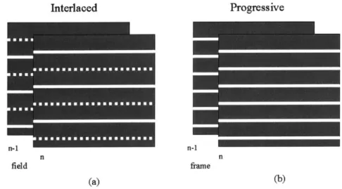
intervals. The scan mode is the method in which the pixels of each frame are displayed. As shown in Figure 1-1, video sequences can have one of two scan modes: progressive or

interlaced. A progressive scan sequence is one in which every line of the video is

scanned in every frame. This type of scanning is typically used in computer monitors and high definition television displays. An interlaced sequence is one in which the display alternates between scanning the even lines and odd lines of the corresponding progressive frames. The standard convention is to start enumeration at zero, i.e. the first line is line 0 and the second line is line 1. Thus, the first line is even and the second line is odd. The

term field is used (rather than frame) to describe pictures scanned using interlaced scanning, with the even field containing all the even lines of one frame and the oddfield containing the odd lines. The terms topfield and bottomfield are also used to denote the even and odd fields, respectively.

Interlaced Progressive

n-i n-i

n n

field frame

(a) (b)

Figure 1-1: Scan modes for video sequences. (a) In interlaced fields either the even or the odd lines are scanned. The solid lines represent the field that is present in the current frame. (b) In progressively scanned frames all lines are scanned in each frame.

While interlacing does succeed in reducing the transmission bandwidth, it also introduces a number of high frequency spatio-temporal artifacts that can be distracting to the human eye, such as line crawl and interline flicker. In addition, there are a number of applications where interlaced scanning is unacceptable. For instance, freeze frame displays and the photographic capture of a television image both require a whole frame to be displayed at once. With advances in technology, it is also becoming more popular to view video on a progressively scanned computer monitor or high definition television set. These applications all require interlaced to progressive conversion. A simple conversion method is to combine the even and odd fields to form a new frame. However, this results in severe blurring in regions of significant motion. The desire to eliminate interlacing

Introduction Chapter I

artifacts provides motivation for developing high quality algorithms for interlaced to progressive conversion, also known as deinterlacing.

One particular application where deinterlacing is very useful is in video surveillance systems. As video recording equipment has become more affordable, the use of video surveillance has become an integral part of security systems worldwide. Nearly every retail store, restaurant, bank, and gas station has some form of video surveillance installed. For the same reasons that interlacing is found throughout broadcast television systems, interlaced scanning is used in the vast majority of security systems as well. The bulk of all existing displays use interlacing in order to facilitate easy interoperability with other interlaced video devices such as cameras, VCRs, or DVD players. Since the rest of the security system is coupled to the display, interlacing is found throughout the video chain. While it is possible that progressively scanned systems may become more commonplace in the future, especially with the recent introduction of HDTV, at the present time nearly every surveillance system uses interlaced scanning.

Typically, when criminal investigators view surveillance footage, they only need to analyze a few frames of interest. They often want to view the frames one at a time, looking for one good image that can help to identify a suspect or analyze a region of interest. Since the video source is interlaced, this type of frame-by-frame analysis is difficult without deinterlacing. Video sequences should be deinterlaced and then analyzed on a high quality, progressively scanned display to improve the intelligibility of the video.

The overall goal of this thesis is to investigate different deinterlacing algorithms to determine methods that will improve the quality and intelligibility of video sequences acquired by surveillance systems. The deinterlacing problem has been studied since interlacing was first introduced, and many different algorithms have been proposed to

Introduction Chapter I

Introduction

deinterlace video sequences in general. However, security video sequences have certain attributes that differentiate them from other sequences. Deinterlacing algorithms for surveillance video sequences do not need to consider a number of characteristics that occur in general video sequences, such as scene changes, global camera motion, or zooming. This greatly simplifies the deinterlacing problem. Secondly, surveillance systems often record video at temporal rates as low as 5 to 10 fields per second. This is significantly lower than the 60 fields per second used in the NTSC standard. As a result of these low temporal rates, adjacent fields are less temporally correlated. Deinterlacing algorithms that rely on this temporal correlation for effectiveness will not work well on this type of video. This thesis will test a number of different deinterlacing algorithms in order to determine which algorithm best fits these characteristics and helps aid in the identification of individuals present in these sequences.

Chapter 2 provides an in depth look at a typical surveillance system. The video analysis methods currently used in practice are also discussed. Formal definitions of interlacing and deinterlacing are provided in Chapter 3. Chapter 4 discusses the deinterlacing algorithms that were examined in this thesis. The advantages and disadvantages of each algorithm are also discussed. One particular class of deinterlacing algorithms showed excellent potential throughout this research. These methods, known as motion adaptive deinterlacing algorithms, are examined in detail in Chapter 5. In addition to the details of the experiments conducted for this thesis, results and analysis are provided in Chapter 6. Finally, Chapter 7 provides the final conclusions and suggestions for further research.

Chapter 2

Surveillance Systems

As video technology has improved, the expense of installing a surveillance system has dropped significantly, leading to an exponential increase in the use of security cameras. Today it is nearly impossible to enter a shopping mall or to eat at a restaurant and not be video taped.

As shown in Figure 2-1, a typical security camera system is made up of three components: the video camera itself, a time-lapse recorder, and a monitor. The video signal flows from the camera to the time-lapse recorder where it is recorded onto a VHS tape. The signal also passes through the recorder to the monitor for possible real-time viewing. Often black-and-white cameras are used to reduce cost, but color cameras are not uncommon. Time-lapse videocassette recorders are essentially high quality VCRs, as can be found in any consumer entertainment system. The only difference is that time-lapse recorders have the ability to record at extremely low temporal rates. The monitor used in this type of system can be any video display, such as a standard television. If a black-and-white camera is used, the monitor is often black-and-white as well, again to help reduce costs. At a given location, there may be many cameras multiplexed into one or more different recorders, but the overall system will be similar to the one depicted in Figure 2-1.

Since the video camera and monitor are both self-explanatory, the component that is really of interest is the time-lapse recorder. These recorders take the video signal from the camera, and record it onto standard VHS tapes. They record the video at very low temporal rates so that the recording time per tape is maximized and fewer tapes are needed. For instance, a standard VHS tape can hold about 8 hours of video using a

Surveillance Systems

standard VCR. However, by using a time-lapse recorder up to 40 hours of video can be recorded on the same tape by recording only 12 fields per second compared to the 60 fields per second recorded by a standard VCR. Requiring the end-user to change videotapes every 8 hours is unacceptable for many surveillance situations, and thus, time-lapse recording makes these surveillance systems feasible. Time-time-lapse recorders give users the ability to select temporal rates much lower than the NTSC standard of 60 fields per second. Rates such as 30 fields per second, 20 fields per second, and 12 fields per second are common.

Video Camera Time-lapse Monitor

Videocassette Recorder

Figure 2-1: A typical security camera system. The video signal is taken from a video camera typically

mounted on a wall or ceiling and recorded with a time-lapse videocassette recorder. The recorded tape can then be viewed later on a monitor.

Once video is recorded onto the VHS tape, it can be played back by the time-lapse recorder and viewed on a monitor. The recorder can play the tape back at the appropriate speed to match the rate at which the video was originally recorded. Since the monitor requires a NTSC signal with a temporal rate of 60 fields per second, the recorder must adjust the output signal. To accomplish this, many recorders use line repetition, the simplest of all deinterlacing algorithms. Line repetition is discussed in more detail in Chapter 4. In the line repetition algorithm, the lines of one field are simply repeated to generate the missing lines and create a whole frame. Figure 2-2 shows an example of using line repetition to convert a 20 field per second signal into a 60 field per second

NTSC signal. The display of a single frame on an interlaced monitor is done in the same

manner, however in this case, a single field is continuously repeated for as long as desired.

VHS Tape

(a)

Video Display

(b)

Figure 2-2: Conversion from VHS storage to NTSC video. (a) Two consecutive fields recorded at 20 fields per second as stored on a VHS tape. (b) Display of the same two fields as an NTSC signal at 60 fields per second. In this example, each field is displayed three times in order to generate a valid NTSC signal. This has the same effect as line repetition, which is discussed in Chapter 4.

Line repetition is one of the simplest methods of deinterlacing and will be shown in later chapters to result in very poor performance. However, this simple algorithm leads to a simple, low-cost implementation. Therefore, line repetition is the method implemented on most time-lapse recorders. For this reason, in most surveillance systems, investigators are forced to view video obtained using line repetition. The remainder of this thesis investigates more advanced methods of deinterlacing the video, so that it may be analyzed with higher intelligibility on progressively scanned displays.

Surveillance Systems Chapter 2

Chapter 3

Deinterlacing

A progressive scan sequence consists of frames, in which every line of the video is

scanned. An interlaced sequence consists of fields, which alternate between scanning the even and odd lines of the corresponding progressive frames. A video sequence is a three-dimensional array of data in the vertical, horizontal, and temporal dimensions. Let

F[x, y, n] denote the pixel in this three-dimensional sequence at horizontal position x,

vertical position y , and time n . Assuming that the video source is progressively scanned, F[x, y, n] is defined for all integers x, y , and n within the valid height, width, and time duration of the sequence. If J,[x,y,n] is an interlaced source generated from the progressive source F[x, y, n], then 1J[x, y, n] is defined as follows

F[x, y, n] mod(y,2)= mod(n,2)

0 otherwise (1)

where the null symbol, 0, represents pixels that do not exist since they are not scanned, and mod(y, 2) is the modulus operator defined as

r0

mod(z,2)={ zodd (2)

Thus, the interlacing operation alternates between selecting the even field or the odd field from the corresponding progressively scanned frame.

Deinterlacing a video sequence involves converting the interlaced fields into progressively scanned frames. Ideal deinterlacing would double the vertical-temporal sampling rate and remove aliasing [5]. However, this process is not a simple rate conversion problem, since the Nyquist criterion requirement is generally not met. Video cameras are not typically equipped with the optical pre-filters necessary to prevent aliasing effects in the deinterlaced output, and if they were, severe blurring would result [5].

For a given interlaced input FJ[x,y,n], the output of deinterlacing, F, [x,y,n], can then

be defined as

F,[x,y,n], mod(y,2)=mod(n,2)

F,[x, y, n] = (3)

F[x, y, n], otherwise

where the pixels F[x, y, n] are the estimation of the missing lines generated by the deinterlacing algorithm. The existing, even or odd, lines in the original fields are directly transferred to the output frame. These definitions will be used throughout this thesis:

F[x, y, n] is the original frame, FI [x, y, n] is the interlaced field, and F, [x, y, n] is the

result of deinterlacing.

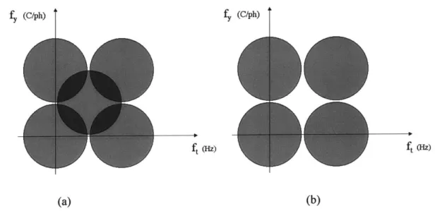
The main difficulty in deinterlacing can be seen in the following figure. Figure 3-1 (a) shows the frequency spectrum of an interlaced signal along the vertical-temporal plane. The interlaced sampling lattice results in the quincunx pattern of spectral repetitions [5]. The darker regions in Figure 3-1 (a) represent aliasing due to the interlaced sampling. The ideal deinterlacing algorithm would remove the central repeated spectra to give the spectrum depicted in Figure 3-1 (b). The areas of overlap in (a) cannot be perfectly recovered by any deinterlacing algorithm, so the result in (b) is not possible in general.

Deinterlacing

f (C/ph) f4 (C/ph)

ft(Hz)

(a) (b)

Figure 3-1: Vertical-temporal spectrum of interlaced video. (a) General vertical-temporal spectrum of

interlaced video sequence. Interlaced sampling causes a quincunx pattern of spectral repetitions. Dark regions represent areas that are unrecoverable due to aliasing. (b) Ideal output of deinterlacing algorithm. Central spectral repetition is removed.

Chapter 3

Chapter 4

Deinterlacing Algorithms

Deinterlacing methods have been proposed ever since the introduction of interlacing. With increases in technology, progressive displays have become feasible and the interest in deinterlacing has increased. The methods that have been suggested vary greatly in complexity and performance, but they can be segmented into two categories: intraframe

and interframe. Intraframe methods only use the current field for reconstruction, while

interframe methods make use of the previous and or subsequent frames as well. Note that, all the methods attempt to reconstruct the missing scan lines without the knowledge of the original progressive source.

The purpose of this thesis is to investigate a number of deinterlacing methods and analyze their performance when applied to surveillance camera footage. To this end, fourteen different algorithms have been compared. Given the extent to which this problem has been studied, it was impossible to implement every algorithm that has ever been suggested. However, these fourteen methods are believed to be a fair representation of the different types of deinterlacing algorithms that have been suggested to date.

The following sections specify the details of the algorithms that were explored as well as their individual advantages and disadvantages.

4.1

Intraframe Methods

Intraframe or spatial methods only use pixels in the current field to reconstruct missing scan lines. Therefore, they do not require any additional frame storage. Initially, the

memory required to store one video frame was expensive, so intraframe methods were attractive. Since spatial methods consider only one frame at a time, their performance is independent of the amount of motion present in the sequence or the frame-recording rate. Robustness to motion is one characteristic that is very useful for deinterlacing low frame rate surveillance video. However, considering only the information in the present field greatly limits these algorithms due to the large temporal correlation that typically exists between successive fields.

4.1.1 Line Repetition

Line repetition is one of the simplest deinterlacing algorithms, and thus, was one of the first to be considered. In this method, the missing lines are generated by repeating the line directly above or below the missing line. The top field is copied down to fill in the missing lines, and the bottom field is copied up as illustrated in Figure 4-1.

Top Field Bottom Field

44 4

ft

f t

t

*0 0

44 4

ft

f t

t

44444

ft

ft

t

Figure 4-1: Illustration of line repetition. The top field is copied down to fill in the missing bottom field. The bottom field is copied up to fill in the missing top field.

Deinterlacing Algorithms Chapter 4

Chapter 4 Deinterlacing Algorithms

The mathematical definition of line repetition is as follows.

For top fields:

[x, y,n] =Fjx,y,n], FF][x,y-l,n],

For bottom fields:

F[x~yn] = J[x, y, n], Fx[x,y+,n], y even otherwise (4) y odd otherwise

An example of the result of line repetition is shown in Figure 4-2.

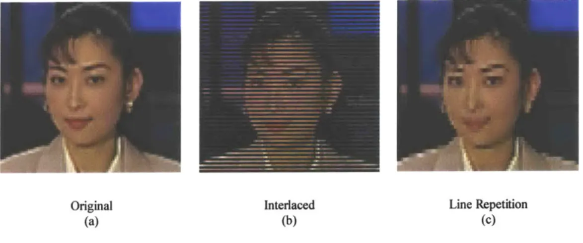
Original

(a)

Interlaced Line Repetition

(b) (c)

Figure 4-2: Example of line repetition. (a) Original progressive frame. (b) Interlaced field. (c) Output of line repetition. The lines in the interlaced field are repeated to generate the output frame.

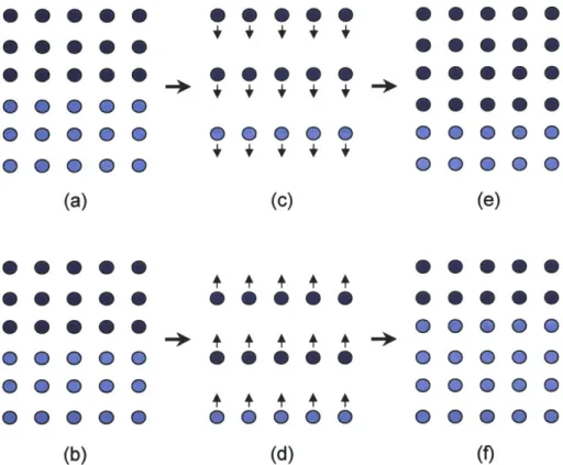
As is shown by the figure, this type of zero-order-hold interpolation often has poor performance. In addition to introducing jagged edge artifacts caused by aliasing, line repetition can also cause severe "jitter" in deinterlaced video due to improper reconstruction of vertical details. A demonstration of the cause of this artifact is shown in Figure 4-3.

Deinterlacing Algorithms Chapter 4

Chapter 4 Deinterlacing Algorithms -0 00 00 + + + + 4 (C) @ 0 @ 0 0 @ S.Q @0Q @0Q 0 0 0 0 0 40 0 0 @ 0 0 @ 0 0 0 0 0 0 0 0 @ 0 0

(a)

(e)

Figure 4-3: Jitter Caused by Line Repetition. (a) (b) Consecutive progressive frames of a stationary image with a horizontal edge. (c) (d) Corresponding interlaced fields. (e) (f) Result of reconstruction using line repetition. Comparing the deinterlaced frames, the incorrect reconstruction of the horizontal edge causes a 2 pixel shift in successive frames. This shift will make the output sequence appear to shake.

As seen in this example, vertical details such as the edge in Figure 4-3 will be incorrectly reconstructed. These errors will make video sequences appear to shake slightly in the vertical direction. The rate of this vibration corresponds directly to the frame rate of the video sequence. At high frame rates, this shaking may be so fast that it becomes unnoticeable to the human eye. However, at lower frame rates this effect becomes very noticeable and extremely annoying.

0 40 0 0 0 0 0 40 @ 0 @ 0 0 0 444444 4 4 4 4 (d) Deinterlacing Algorithms Chapter 4

Deinterlacing Algorithms

4.1.2 Linear Interpolation

Linear interpolation is another simple deinterlacing algorithm that is only slightly more advanced than line repetition. In linear interpolation the missing lines are reconstructed

by averaging the lines directly above and below. The formal definition of linear interpolation is

[F[x,y,n] , mod(y,2)=mod(n,2)

F[x,y,n]= F,[x,y+l,n]+F,[x,y-l,n] (5)

, otherwise

This type of algorithm results in a slightly smoother picture than line repetition, but still has fairly poor performance. The same problems caused by line repetition, such as aliasing artifacts and jitter, exist with linear interpolation as well.

4.1.3 Parametric Image Modeling

A more advanced form of spatial deinterlacing utilizes image modeling. Parametric

image modeling algorithms attempt to model a small region of an image through a set of parameters and basis equations. Missing lines are reconstructed using linear interpolation. The model attempts to determine the contours of a shape in an image and interpolates along this direction to reduce interpolation errors. Martinez and Lim, and Ayazifar and Lim have suggested models, which can be used to spatially interpolate, interlaced video fields. Martinez suggests a Line Shift Model in which small segments of adjacent scan lines are assumed to be related to each other through a horizontal shift [18]. Ayazifar similarly suggests a generalization of the Line Shift Model through a Concentric Circular Shift Model in which small segments of concentric arcs of an image are related to adjacent arcs by an angular shift [1].

Deinterlacing Algorithms

One of the benefits of these methods is that they tend to be less susceptible to noise. When attempting to fit an image to a model, pixels corrupted by noise often do not correctly fit the within the model, and thus the model tends to disregard them. However, the system must also be over-determined in order for the model to closely match the actual image, which requires considering a large area of the image as well as more computations. Depending on the order of model selected, the complexity of this algorithm can be greater than other methods.

The Line Shift Model method suggested by Martinez and Lim has been included in this study [18]. Figure 4-4 illustrates the general idea of this algorithm. The algorithm begins

by selecting a certain group of pixels surrounding the missing pixel that is to be

reconstructed. The algorithm implemented for this study uses a group of 10 pixels, 5 pixels on two lines, as suggested by Martinez in [18]. The parameters for the image model are then estimated for the selected group of pixels, and these parameters are used to estimate the appropriate line shift vector. Once the shift vector is determined, interpolation is done along the direction of the estimated line shift as is shown in Figure 4-5.

Estimate

Current Field 0 Select Model

Samples _Parameters

Calculate Line Shift

Interpolate Output Pixel

Figure 4-4: Implementation of Martinez-Lim spatial deinterlacing algorithm

Chapter 4 Deinterlacing Algorithms

Missing Field Line - Q Q Q Q Q -Known Field Lines

0 0 0 0

4--Figure 4-5: Interpolation by Martinez-Lim algorithm. Appropriate line shift is calculated and interpolation is done along this direction. In this example, the missing pixel at the center of the figure is reconstructed by averaging the two pixels along the edge direction.

A comparison of the spatial deinterlacing algorithms that have been mentioned is shown

in Figure 4-6. Of these three, the Martinez-Lim algorithm tends to generate the

smoothest, most realistic images. While it also suffers from some of the jitter effects found in line repetition, these effects are significantly reduced when compared to the other two methods.

(a) (b) (c)

Figure 4-6: Comparison of intraframe interpolation methods. (a) Line repetition. (b) Linear

interpolation. (c) Martinez-Lim algorithm.

Deinterlacing Algorithms Chapter 4

4.2

Interframe Methods

While the performance of spatial methods is independent of the amount of motion present in an image, they essentially ignore a significant amount of information in adjacent frames that may be useful. For instance, if a video sequence contains one perfectly stationary image, this sequence could be perfectly deinterlaced by simply combining the even and odd fields. Interframe or temporal methods consider previous and/or subsequent frames to exploit temporal correlation. These methods require storage for one or more frames in their implementation, which may have been a serious difficulty in the past. However, the cost of frame storage is not as serious an issue with the reduced cost of memory.

4.2.1 Field Repetition

Field repetition refers to the generation of missing scan lines by copying lines from the previous frame at the same vertical position. Specifically, field repetition is defined as:

{[x,y,n],

,, Ji[x,y,n-1], otherwise

This type of deinterlacing would provide essentially perfect reconstruction of stationary video. However, field repetition can cause severe blurring if the video contains motion. Consider the example presented in Figure 4-7.

At high frame rates, the temporal correlation between two adjacent fields may be very high. If this is the case, field repetition can perform well with minor noticeable blurring. Yet, at lower temporal rates, as is used in surveillance video, this blurring effect becomes

more pronounced. Figure 4-8 shows an example of the effects of field repetition being used in a moving region of a video sequence.

Stationary Even Field Time 1 Odd Fieldl Time 2 Field Repetition Moving Even Field Time 1 Odd Field Time 2 Field Repetition

Figure 4-7: Example of deficiency in field repetition algorithm. The stationary circle is perfectly

reconstructed by combining the even and odd fields. However, in the second example, the image is blurred since the even and odd fields are no longer properly aligned due to the motion of the circle between frames.

(a) (b)

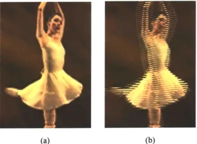
Figure 4-8: Blurred frame caused by field repetition. (a) Original progressive frame. (b) Frame produced using field repetition. Motion of the ballerina causes edges to be distorted resulting in a blurred image.

Deinterlacing Algorithms

Since surveillance video systems use stationary video cameras, most regions of the video contain no motion. For instance, the background regions, where no motion is taking place, make up the majority of these video sequences. In these regions, field repetition will have excellent performance. Yet, given the extremely low frame rates used in surveillance video, field repetition can cause severe artifacts wherever motion is present. Thus, it is not suitable for this application, since the areas of motion are likely to be the main areas of interest. However, it was included in this study for comparison purposes.

4.2.2 Bilinear Field Interpolation

Bilinear field repetition uses the average of the previous and future lines to deinterlace the current missing line. The formal definition is

F[x,y,n] , mod(y,2)=mod(n,2)

F[x,y,n]= F[x, y,n+1]+JF[x,y,n-1] (7)

1.

Field interpolation has essentially the same benefits and issues as field repetition. This method works very well in stationary regions, and works poorly in moving regions. Field interpolation actually introduces more blurring artifacts in the presence of motion since it blends three frames together rather than just two. Figure 4-9 shows an example of this distortion. The three separate fields are each visible in image (b). The current field shows up in the center with the strongest color. The previous and future fields show up, slightly blended into the background. The result is a "ghostly" image with badly blurred edges. In this sense, when compared to field repetition, field interpolation is even more unacceptable.

Chapter 4 Deinterlacing Algorithms

(a) (b)

Figure 4-9: Blurred frame caused by field interpolation. (a) Original progressive frame. (b) Frame produced using bilinear field interpolation. Three fields of the video sequence are blended together leaving a severely distorted result in the presence of motion.

4.2.3 Vertical-Temporal Median Filtering

As with all interframe methods Vertical-Temporal (VT) filters use pixels in adjacent frames, however VT filters also utilize neighboring pixels in the current frame. In VT median filtering, as its name implies, a median operation is used rather than a linear combination of the surrounding pixels. VT median filtering has become very popular due to its performance and ease of implementation. The simplest example of a VT median filter is the 3-tap algorithm as suggested in [5]. To calculate the pixel X as seen in Figure

4-10, one simply finds the median of the two vertically adjacent points, A and B, and the

temporally adjacent point in the previous field, C, as described in (8).

Deinterlacing Algorithms Chapter 4

Chapter 4 Deinterlacing Algorithms

n-i n

field number

Figure 4-10: Pixel definitions for 3-tap VT Median Filtering

X = med(A, B, C) (8)

This is formally described as

F ri =f[J~F[x,y,n] , mod(y,2)=mod(n,2)

[x, y

median(F [x,y+1,n],

Median filtering adapts itself to moving and stationary regions on a pixel-by-pixel basis.

If the image is stationary, pixel C is likely to take on a value somewhere between A and

B. Thus, pixel C will be chosen by the median operation resulting in temporal filtering. If the region is moving, pixel C is likely to be very different than A or B, and thus, A and B will typically have a higher correlation with each other than with pixel C. The median filter will then select either pixel A or pixel B resulting in spatial filtering. A number of variations on this median filter have been suggested. For instance, filters with more taps have been used such as the seven-tap filters suggested by Salo et al [21] or Lee et al [15].

Deinterlacing Algorithms Chapter 4

Deinterlacing Algorithms

For this research two median filters have been implemented; the three-tap median filter as presented in (9), and a modification of the seven-tap weighted median filter presented by Lee et al [15]. In their weighted median filter, the following median operation is implemented.

Let

A=J [x,y-1,n] E=A+B

2

B=F [x,y+1,n] F =C+D

2

C =

F,

D=i, [x,y,n+1]

F [x,

[x,

median(A, B, C, D, E, E, F) , otherwise

Again, this type of median filter will be robust to motion and will be likely to select a spatial deinterlacing method in the presence of motion. However, in the presence of motion, linear interpolation (pixel E) becomes somewhat more likely than line repetition (pixels A and B) since pixel E is given twice as much weight in the median filter.

4.2.4 Motion Compensated Deinterlacing

The most advanced techniques for deinterlacing generally make use of motion estimation and compensation. There are many motion estimation algorithms that can be used to estimate the motion of individual pixels between one field and then next. If accurate motion vectors are determined, motion compensation (MC) can basically remove the motion from a video sequence. If motion were perfectly removed, temporal interpolation could theoretically restore the original frames. However, motion vectors are often

incorrect and any motion compensated deinterlacing methods have to be robust enough to account for this. In general any non-MC algorithm can be converted to a MC algorithm.

However, only those techniques that perform better on stationary images will most likely be improved. Some straightforward MC methods include field repetition, field

interpolation, and VT median filtering.

The most common method for determining motion vectors is through block matching algorithms. The image is segmented into blocks, for instance, 8x8 blocks of pixels are fairly common, and then each of those blocks is compared to the previous frame in a given search area, such as -15/+16 pixels in both the horizontal and vertical directions. The block within the search area, which most closely "matches" the original block, is selected to compute the motion vector. The "matching" criterion that is typically used is either mean square error or mean absolute error. There are a number of variations on this algorithm that involve different search regions or different criteria for selecting the most closely matching block. Other algorithms have been used which use phase correlations of adjacent frames to determine shifts of objects within the frames. The two-dimensional Fourier transforms for the two fields are calculated and a phase correlation surface is determined. From this surface it is possible to locate peaks corresponding to shifts of objects from one frame to the next, and map these shift back onto the original field.

A number of problems can arise when using this type of motion estimation scheme. For

instance when objects pass in front of one another, there are appearing and disappearing regions of the fields, which cannot be accounted for with motion vectors. Also, if an object moves beyond the motion vector search area, the motion vector will not be accurately determined. Another fundamental problem with motion compensation is that the pixels may have sub-pixel motion. In this case, the motion vector actually should point between pixels or at missing lines in the previous field. In the horizontal direction, the video is assumed to be sampled at a high enough rate that the general sampling

theorem can be used to correctly interpolate the needed value. However, in the vertical direction, the data is sub-sampled and band limited interpolation will not provide an appropriate result.

In the general deinterlacing problem, motion compensation can be used to compensate for translational motion of static objects, meaning objects that shift from one position to another without deforming or changing shape. Thus, motion compensation can be very effective when deinterlacing a video sequence acquired from a panning camera. However, this type of motion seldom occurs in surveillance situations that use a stationary camera. The objects that are static, such as walls and doors, are not moving because the camera is not moving. The objects that do move are not static; they are typically individuals who change shape quite often. This type of motion is not translational, and is thus beyond the scope of the two-dimensional translational model. In this type of situation, accurate motion vectors cannot be found, since they do not exist. This problem is compounded by the low temporal rates used in these sequences, which decreases temporal correlation between adjacent frames.

This thesis looks at three different methods that use motion compensation: field repetition, field interpolation, and a three-tap VT median filter. Half-pixel motion estimation algorithms were used with 8x8 blocks and a search range of -31/+32 pixels. The large search range was selected because of the large amounts of motion that are possible between successive frames due to the low temporal recording rates.

4.2.5 Motion Adaptive Deinterlacing

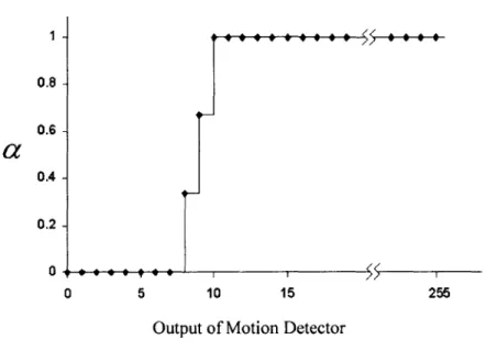
Interlaced sequences can be essentially perfectly reconstructed by interframe methods in the absence of motion, while intraframe methods perform well in the presence of motion [25]. Motion adaptive methods use a motion detector to take advantage of this fact by separating each field into moving and stationary regions. Based on the output of the

motion detector, the deinterlacing algorithm then fades between a temporal method that works well for stationary images and a spatial method for moving images. The output of this type of motion adaptive algorithm can be represented as in (11) where a represents a motion detection parameter that indicates the likelihood of motion for a given pixel

_F

[x,

a- F,,,, [x,y,n]+(1-a).Fsat[x,y,n], otherwise

The pixels F,,, (x, y, t) are calculated for stationary regions using a temporal method, and the pixels F,,,,, (x, y, t) are calculated for moving regions using a spatial method.

Preliminary results indicated that motion adaptive methods had the most potential for use with low frame rate surveillance video. Motion adaptive methods correspond well with surveillance video. For example, the majority of these sequences consist of stationary background type regions due to the stationary camera system. These background areas can be deinterlaced using field repetition or interpolation with very high accuracy. Another benefit of motion adaptive methods is that their performance is not significantly degraded when used on sequences with low frame rates. For these reasons, motion adaptive methods were given the most attention during this study. The details of motion detection and motion adaptive methods are examined in detail in the following chapter.

Chapter

5

Motion Adaptive Deinterlacing

Motion adaptive deinterlacing methods are designed to take advantage of the varying information that is present in different regions of a video sequence. In stationary images, there exists significant correlation between the present field and the adjacent fields. Temporal methods such as field repetition are designed to benefit from this fact. In moving regions, this temporal correlation does not exist, and more information can be found in adjacent pixels on the current field. Spatial methods take advantage of this fact. Motion adaptive deinterlacing attempts to combine the benefits of both temporal and spatial methods by segmenting each image into moving and stationary regions. Stationary regions are reconstructed with a temporal method while moving regions are reconstructed with a spatial method.

In order to segment a video sequence into moving and stationary regions, motion adaptive methods must use some form of motion detection. The next section covers some of the issues with detecting motion in interlaced sequences and describes the different algorithms that were implemented in this study.

5.1

Motion Detection in Interlaced Sequences

The goal of motion detection is to detect changes in a video sequence from one field to the next. If a significant change is detected, that region declared to be moving. If no significant changes are detected the region is assumed to be stationary. This task is straightforward for a progressive sequence. A simple frame difference can be used to detect changes and a threshold can be applied to indicate the presence or absence of motion. An example of this idea is shown in Figure 5-1.

Chapter 5 Motion Adaptive Deinterlacing (a) (b) CIL ~ .

AL

Figure 5-1: Example of motion detection using progressive frames. (a) (b) Two successive frames from a video sequence. (c) Result of absolute frame difference. Result of frame differencing can be used as an indication of the presence or absence of motion.

Frame differencing cannot be used for interlaced sequences. In fact, it is impossible since consecutive fields do not have the same pixel locations, i.e. an even field cannot be subtracted from an odd field since the corresponding pixels do not exist. The following sections discuss some of the proposed solutions for motion detection in interlaced sequences.

Motion Adaptive Deinterlacing Chapter 5

5.1.1 Two-Field Motion Detection

The simplest approach to interlaced motion detection is to convert the fields to frames, using any deinterlacing method. Once the fields have been deinterlaced, motion detection is straightforward, and can be performed as in the progressive case discussed above [17]. Any spatial deinterlacing method can be used for this purpose, such as line repetition, linear interpolation, or the Martinez-Lim algorithm. Figure 5-2 illustrates this idea.

* 0

*

0

n-2 n-i n n+1 n+2

Time

Figure 5-2: Two-field motion detection scheme for determining the presence or absence of motion at pixel location 'X'. The dark circles represent pixels in a video sequence on different scan lines at the same horizontal position. The pixel at location 'X' is interpolated, represented in the picture by the light circle, and then an absolute difference is computed between the interpolated pixel and the pixel from the previous field.

This figure depicts five separate fields of a video sequence. The dark circles symbolize pixels on varying scan lines at the same horizontal position. The alternating odd and even fields can be seen in this figure. Suppose the location 'X' is the pixel for which motion is being estimated. In two-field motion detection the pixel at location 'X' is interpolated spatially, which is represented here by the light-colored circle. Then an absolute difference is computed between the interpolated pixel and the pixel from the previous field. This pixel difference is represented in this figure by the double arrow symbol.

_ - 0 1- & ' L

Motion Adaptive Deinterlacing Chapter 5

A more theoretical approach to this problem is presented by Li, Zeng, and Liou [17].

Since the difference between an even sampled field and an odd sampled field is a phase shift, they suggest applying a phase correction filter to one field so that it may be more appropriately compared with the opposite polarity field for motion detection. They use the following 6-tap filter for phase correction of the current frame:

F0[x y n =F

[x,

F,[x~~n]=(12)

3-Fi[x,y,n 5]-21Fi[x,y,ni3]+147-Fi[x,y,n ], otherwise

Obviously, their method does not result in perfect reconstruction, since it is unable to remove the aliasing terms. However, this method does provide an interesting theoretical solution to the problem through an application of sampling theory. Their method also showed the best performance over the other spatial deinterlacing methods for use in this type of two-field motion detection and was used for two-field motion detection in this study.

The problem that arises with two-field motion detection is that, without perfect reconstruction, there will be some errors made in the interpolation step. These errors can make vertical details in the picture appear as motion. For instance, the pixels above and below pixel 'X' in Figure 5-2 do not necessarily have any correlation to the actual value of pixel 'X'. Thus, the interpolation may be done incorrectly and the absolute difference will not be an appropriate measure of motion. Thus, motion may be detected when none was present. This error leads to a significant number of false-detections. As a result, more regions of the video sequence will be deinterlaced spatially than necessary, resulting in lower quality.

5.1.2 Three-Field Motion Detection

The only way to avoid the problems introduced by two-field motion detection is to only compare pixels on identical lines. For instance, no interpolation should be done in order to compare two pixels that are not on corresponding lines. With this in mind, the simplest method of motion detection is a three-field motion detection scheme suggested in [15] and presented in Figure 5-3.

This figure is similar to Figure 5-2, except that no interpolation is needed, and so the light colored pixel is omitted. Assume that motion is being detected for the location marked

by the symbol 'X'. In a three-field motion detection scheme, the pixel in the previous

field is compared to the same pixel in the next field. Since the previous and the next field have the same spatial location, the absolute difference can be computed without any interpolation. An absolute difference of these two pixels is computed as an indication of the likelihood of motion.

0 0

~ S 0

n-2 n-1 n n+1 n+2 Time

Figure 5-3: Three-field motion detection scheme for determining the presence or absence of motion at pixel location 'X'. An absolute difference is computed between the pixel in the previous frame and the pixel in the next frame. Only pixels on corresponding scan lines are compared, so no interpolation is needed.

While two-field motion detection results in many false alarms (detecting motion when none is present), three-field motion detection results in many missed detections (not

Motion Adaptive Deinterlacing Chapter 5

detecting motion when motion actually is present) because it is unable to detect fast moving regions. The following example illustrates an example of a missed detection when utilizing three-field motion detection.

(a) (b) (c)

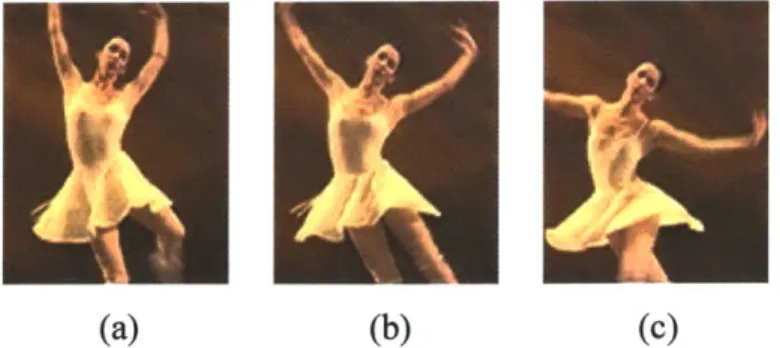
Figure 5-4: Sequence of frames which will cause three-field motion detection to fail.

Figure 5-4 presents three sequential frames of a video sequence. In Figure 5-4 (b), consider the ballerina's left arm. In this example, the three-field motion detection scheme would incorrectly label this area as stationary. In this region, images (a) and (c) look exactly alike. This motion detection algorithm will compare (a) with (c), assume that nothing has changed in that particular region, and label it as stationary. The result of deinterlacing using these erroneous motion detection parameters can be found in Figure 5-5.

Figure 5-5: Results of motion adaptive deinterlacing when errors are made in motion detection

Motion Adaptive Deinterlacing Chapter 5

The artifacts caused by missed detection are similar to those caused by field repetition. The dancer's left arm is blurred out, leaving only a ghostly outline. The same artifact occurs in other regions of this image for identical reasons.

5.1.3 Four-Field Motion Detection

In an attempt to improve upon three-field motion detection by reducing the number of missed detections, one can use a four-field motion detection algorithm [15]. The idea behind four-field motion detection is presented in Figure 5-6.

a) U ci) 0 +-n-2 0 0 n-I - 0 x 0 n Time 0 n+I 0 0 n+2

Figure 5-6: Four-field motion detection scheme for determining the presence or absence of motion at pixel location 'X'. Three absolute differences are computed. This results in a better detection of fast motion. Only pixels on corresponding scan lines are compared, so no interpolation is needed.

In this scheme, three pixel comparisons are used rather than the one set of pixels that are compared in the previous two algorithms. The additional two pixel differences help to protect against the error that was demonstrated in Figures 5-4 and 5-5. Figure 5-7 shows the final result after this error has been corrected.

Motion Adaptive Deinterlacing Chapter 5

Chapter 5 Motion Adaptive Deinterlacing

Figure 5-7: Results of motion adaptive deinterlacing using four-field motion detection. Missed detections that were made by the three-field motion detection have been removed.

The output of this motion detector is the maximum of the three pixel differences.

A=

1F

₁

B =

IF,

2]I

C = }F

[x,

[x,

motiondetected = max (A, B, C) (13)

While this method has better performance than three-field motion detection, it can still miss detections. The occurrences are far less likely, but they can occur. The following sequence of sequential frames demonstrates an example where four-field motion detection claims a region is stationary when motion is actually present.

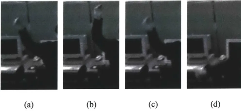
(a) (b) _(c) (d)

Figure 5-8: Sequence of frames which will cause four-field motion detection to fail.

Motion Adaptive Deinterlacing Chapter 5

Chapter 5 Motion Adaptive Deinterlacing

In this sequence, consider the position of the waving hand in frame (c). In frame (a) the hand is also approximately in the same position. The two frames are not identical, but at least some regions of the hand and arm are similar. The four field motion detection will compare frames (a) and (c) and will assume that nothing has changed for the majority of the pixels. Similarly, the algorithm will perform a comparison of frames (b) and (d). While these frames (b) and (d) are clearly very different, they are nearly identical in the area in question, so the algorithm will assume nothing has changed in that region either. The end result will be that no motion will be detected in this area, while frame (c) and frame (b) are quite different. The effects of this type error are similar to that shown in Figure 5-5.

5.1.4 Five-Field Motion Detection

The final motion detection algorithm that was investigated is a five-field based method that was suggested by the Grand Alliance, developers of the United States HDTV standard, for HDTV format conversion [2]. This method improves upon four-field motion detection by reducing the number of missed motion detections. The method they propose is illustrated in Figure 5-9.

0

0

0

* 0

n-2 n-I n n+1 n+2

Time

Figure 5-9: Five-field motion detection scheme for determining the presence or absence of motion at pixel location 'X'. A weighted combination of five absolute differences is used.

Let

A=

IF,

i]

B =

IF,

C =IF [x,y+1,n]-F

_[x,y+1,n-2]!

D =

IF,

E =

IF,

The output of this motion detector is then the following combination of these five pixel differences.

motiondetected = max A, B+C D+E (14)

2 2

In this maximum operation, the two pixel differences between the fields at time n and n-2 are averaged, and the two pixel differences between the fields at n and n+2 are averaged.

This method also allows for one additional improvement. The previous methods, with the exception of the three-field motion detector, look for motion in one direction in time. In particular, they are all orientated to find differences between the current frame and the previous frames. Thus these methods will all use the previous field for temporal deinterlacing. However, the five-field method, in some sense, looks for motion in both the forward and backward directions. Thus it is not immediately clear whether the motion adaptive deinterlacing algorithm should use the previous field or the next field for temporal interpolation. In this case, a type of median filter is used for temporal deinterlacing, as suggested by the Grand Alliance, the following median operation is used

for temporal deinterlacing [2].