2013 — Low-complexity high prediction accuracy visual quality metrics and their applications in H.264/AVC encoding mode decision process

ÉCOLE DE TECHNOLOGIE SUPÉRIEURE UNIVERSITÉ DU QUÉBEC

THESIS PRESENTED TO

ÉCOLE DE TECHNOLOGIE SUPÉRIEURE

IN PARTIAL FULFILLMENT OF THE REQUIREMENTS FOR THE DEGREE OF DOCTOR OF PHILOSOPHY

Ph. D.

BY

Soroosh REZAZADEH

LOW-COMPLEXITY HIGH PREDICTION ACCURACY VISUAL QUALITY METRICS AND THEIR APPLICATIONS IN H.264/AVC ENCODING MODE DECISION PROCESS

MONTREAL, OCTOBER 9, 2013 © Copyright 2013 reserved by Soroosh Rezazadeh

© Copyright reserved

It is forbidden to reproduce, save or share the content of this document either in whole or in parts. The reader who wishes to print or save this document on any media must first get the permission of the author.

BOARD OF EXAMINERS (THESIS PH.D.) THIS THESIS HAS BEEN EVALUATED BY THE FOLLOWING BOARD OF EXAMINERS

Mr. Stéphane Coulombe, Thesis Supervisor

Department of Software and IT Engineering at École de technologie supérieure

Mr. Mohamed Cheriet, President of the Board of Examiners

Department of Automation Engineering at École de technologie supérieure

Mr. Pierre Dumouchel, Examiner

Department of Software and IT Engineering at École de technologie supérieure

Mr. Guillaume-Alexandre Bilodeau, External Examiner

Department of Computer Engineering at École Polytechnique de Montréal

THIS THESIS WAS PRENSENTED AND DEFENDED

IN THE PRESENCE OF A BOARD OF EXAMINERS AND PUBLIC ON SEPTEMBER 6, 2013

ACKNOWLEDGMENTS

It would not be possible to complete this PhD thesis without the aid and support of many people over the past years. First and foremost I want to express my gratitude and appreciation towards my supervisor, Prof. Stéphane Coulombe, for his support, thoughtful guidance, useful comments, remarks, and engagement throughout the entire learning process of this PhD thesis. I am grateful to him for giving me the opportunity to become a member of his research group. I also thank the other committee members who have accepted to devote their precious time to evaluating my thesis.

My thanks go also to the members of the jury, Professors Mohamed Cheriet, Pierre Dumouchel, and Guillaume-Alexandre Bilodeau, who have accepted to devote their precious time to evaluating my thesis.

Guillaume-Alexandre Bilodeau, who have accepted to devote their precious time to evaluating my thesis.

I would like to convey my thanks to my friends, including the current and former members of our research group, who helped and provided me a supportive and enjoyable environment in the past years.

I should mention that this research was made possible by the support of Vantrix Corporation and the Natural Sciences and Engineering Research Council of Canada (NSERC) who funded this work under the Collaborative Research and Development Program (NSERC-CRD 326637-05).

Finally, I owe my deepest gratitude to my beloved family, whose boundless love and continuous support and encouragement was the source of inspiration to finish this work.

MÉTRIQUES DE QUALITÉ VISUELLE À HAUTE EXACTITUDE ET À FAIBLE COMPLEXITÉ DE CALCULS ET LEUR APPLICATION AU PROCESSUS DE

DÉCISION DE MODES DE L’ENCODEUR H.264/AVC Soroosh REZAZADEH

RÉSUMÉ

Dans cette thèse, nous développons un nouveau cadre général pour calculer des métriques de qualité d’image avec référence complète dans le domaine des ondelettes discrètes en utilisant l'ondelette de Haar. Le cadre proposé présente un excellent compromis entre l’exactitude et la complexité. Dans notre cadre, les métriques de qualité sont classées soit à base de cartes (map), qui génèrent une carte de qualité (distorsion) dont la contribution à chaque position est mise en commun pour le calcul de la métrique finale, par exemple, la similarité structurelle (SSIM), ou non basées sur des cartes, qui calculent directement la métrique finale, par exemple, le rapport signal sur bruit de crête (PSNR). Pour les métriques basées sur des cartes, le cadre proposé définit une carte de contraste dans le domaine des ondelettes pour la mise en commun des cartes de qualité.

Nous développons aussi une formule permettant de calculer automatiquement le niveau de décomposition en ondelettes approprié pour les métriques basées sur l'erreur en tenant compte de la distance de visualisation désirée. Pour tenir compte de l'effet des détails très fins de l'image dans l'évaluation de la qualité, la méthode proposée définit une carte de contours multi-niveau pour chaque image, qui ne comprend que les sous-bandes d'images les plus informatives.

Pour clarifier l'application du cadre dans le calcul de métriques, nous donnons quelques exemples montrant comment le cadre peut être appliqué pour améliorer la performance de métriques bien connues telles que le SSIM, la fidélité de l'information visuelle (VIF), le PSNR, et la différence absolue. Nous comparons la complexité des différents algorithmes obtenus par le cadre à l’encodage H.264 avec profil de base en utilisant l’implémentation IPP en C/C++ d’Intel. Nous évaluons la performance globale des mesures proposées, y compris leur exactitude de la prédiction, sur deux bases de données de qualité d'image bien connues et une base de données de qualité vidéo. Tous les résultats des simulations confirment l'efficacité du cadre proposé et les mesures d'évaluation de la qualité dans l'amélioration de l’exactitude de la prédiction et aussi la réduction de la complexité de calcul. Par exemple, en utilisant le cadre, nous pouvons calculer le VIF avec environ 5% de la complexité de sa version originale, mais avec une plus grande précision.

Dans la prochaine étape, nous étudions comment le processus de décision de modes de codage en H.264 peut bénéficier des métriques développées. Nous intégrons la métrique SSEA proposée comme mesure de distorsion dans le processus de décision de mode H.264.

de validation. Nous proposons un algorithme de recherche pour déterminer la valeur du multiplicateur de Lagrange pour chaque paramètre de quantification (QP). La recherche est appliquée sur trois différents types de séquences vidéo présentant diverses caractéristiques au niveau de l'intensité du mouvement, et les valeurs du multiplicateur de Lagrange qui en résultent sont compilées pour chacun d'eux. Sur la base de notre cadre proposé, nous proposons une nouvelle métrique de qualité PSNRA, et nous l'utilisons dans cette partie (la

décision de mode). Les courbes débit-distorsion (RD) simulées montrent que pour le même PSNRA, avec la décision de mode basée SSEA, le débit est réduit d'environ 5% en moyenne

par rapport à l'approche traditionnelle basée SSE sur les séquences avec des niveaux d’intensité de mouvement faibles et moyens. Il est à noter que la complexité de calcul n'est aucunement augmentée en utilisant l'approche basée SSEA proposée au lieu de la méthode

traditionnelle basée SSE. Par conséquent, l'algorithme de décision de mode proposé peut être utilisé pour le codage vidéo en temps réel.

Mots-clés: transformée en ondelettes discrète, évaluation de qualité d'image, système visuel humain (HVS), fidélité de l'information, similarité structurelle, encodage vidéo, H.264, multiplicateur de Lagrange

LOW-COMPLEXITY HIGH PREDICTION ACCURACY VISUAL QUALITY METRICS AND THEIR APPLICATIONS IN H.264/AVC ENCODING MODE

DECISION PROCESS Soroosh REZAZADEH

ABSTRACT

In this thesis, we develop a new general framework for computing full reference image quality scores in the discrete wavelet domain using the Haar wavelet. The proposed framework presents an excellent tradeoff between accuracy and complexity. In our framework, quality metrics are categorized as either map-based, which generate a quality (distortion) map to be pooled for the final score, e.g., structural similarity (SSIM), or non based, which only give a final score, e.g., Peak signal-to-noise ratio (PSNR). For map-based metrics, the proposed framework defines a contrast map in the wavelet domain for pooling the quality maps.

We also derive a formula to enable the framework to automatically calculate the appropriate level of wavelet decomposition for error-based metrics at a desired viewing distance. To consider the effect of very fine image details in quality assessment, the proposed method defines a multi-level edge map for each image, which comprises only the most informative image subbands.

To clarify the application of the framework in computing quality scores, we give some examples showing how the framework can be applied to improve well-known metrics such as SSIM, visual information fidelity (VIF), PSNR, and absolute difference. We compare the complexity of various algorithms obtained by the framework to the Intel IPP-based H.264 baseline profile encoding using C/C++ implementations. We evaluate the overall performance of the proposed metrics, including their prediction accuracy, on two well-known image quality databases and one video quality database. All the simulation results confirm the efficiency of the proposed framework and quality assessment metrics in improving the prediction accuracy and also reduction of the computational complexity. For example, by using the framework, we can compute the VIF at about 5% of the complexity of its original version, but with higher accuracy.

In the next step, we study how H.264 coding mode decision can benefit from our developed metrics. We integrate the proposed SSEA metric as the distortion measure inside the H.264

mode decision process. The H.264/AVC JM reference software is used as the implementation and verification platform. We propose a search algorithm to determine the Lagrange multiplier value for each quantization parameter (QP). The search is applied on three different types of video sequences having various motion activity features, and the resulting Lagrange multiplier values are tabulated for each of them. Based on our proposed framework we propose a new quality metric PSNRA, and use it in this part (mode decision). The

simulated rate-distortion (RD) curves show that at the same PSNRA, with the SSEA-based

SSE-based approach for the sequences with low and medium motion activities. It is notable that the computational complexity is not increased at all by using the proposed SSEA-based

approach instead of the conventional SSE-based method. Therefore, the proposed mode decision algorithm can be used in real-time video coding.

Keywords: discrete wavelet transform, image quality assessment, human visual system (HVS), information fidelity, structural similarity, video encoding, H.264, Lagrange multiplier

TABLE OF CONTENTS

Page

INTRODUCTION ...1

CHAPTER 1 DIGITAL IMAGE AND VIDEO QUALITY ASSESSMENT MODELS AND METRICS...7

1.1 Introduction ...7

1.2 Bottom-up approaches for visual quality assessment ...10

1.3 Top-down approaches for visual quality assessment ...11

1.3.1 Structural similarity approach ... 11

1.3.2 Information-theoretic approach ... 16

1.4 Discussion ...17

CHAPTER 2 THE PROPOSED LOW-COMPLEXITY DISCRETE WAVELET TRANSFORM FRAMEWORK FOR FULL REFERENCE IMAGE QUALITY ASSESSMENT ...19

2.1 Motivation ...19

2.2 The proposed discrete wavelet domain image quality assessment framework ...20

2.3 Examples of framework applications ...27

2.3.1 Structural SIMilarity ... 28

2.3.2 Visual information fidelity ... 30

2.3.2.1 Scalar GSM-based VIF ... 30

2.3.2.2 Description of the computational approach ... 32

2.3.3 PSNR... 34

2.3.4 Absolute difference (AD) ... 39

CHAPTER 3 THE PERFORMANCE EVALUATION OF THE PROPOSED VISUAL QUALITY ASSESSMENT FRAMEWORK ...43

3.1 Computational complexity of the algorithms ...43

3.2 Verification of quality prediction accuracy of metrics for images ...46

3.3 Verification of quality prediction accuracy of metrics for videos ...54

3.4 Conclusion ...55

CHAPTER 4 MODE DECISION IN H.264 VIDEO ENCODING CONSIDERING THE HUMAN VISUAL SYSTEM ...57

4.1 Background and related works...57

4.1.1 Inter prediction and macroblock partitions in H.264 ... 57

4.1.2 Rate distortion optimized mode selection in H.264 ... 59

4.1.2.1 Lagrange multiplier estimation for mode decision ... 59

4.1.2.2 The conventional process of encoding a macroblock ... 68

4.1.3 Adaptive and HVS-based Lagrange multiplier estimation in RDO for video coding ... 74

4.1.3.2 HVS-based Lagrange multiplier calculation techniques ... 77

CHAPTER 5 THE PROPOSED PERCEPTUAL RDO BASED MODE DECISION USING LOW COMPLEXITY HVS RELATED DISTORTION METRICS ...89

5.1 Motivation ...89

5.2 The proposed approach for perceptual coding mode decision ...91

5.2.1 Theoretical analysis of macroblock distortions relationship ... 93

5.2.2 Simulation conditions ... 95

5.2.3 Empirical analysis of macroblock distortion measures ... 97

5.3 The proposed search method for empirical determination of the Lagrange multiplier λp ...106

5.4 Simulated rate-distortion curves ...109

5.4.1 RD curves when λMOTION = λMODE ... 109

5.4.2 RD curves when λMOTION ≠ λMODE ... 117

5.4.3 RD curves for non-adapted Lagrange multiplier λp ... 121

5.5 Conclusion and future research ...122

CHAPTER 6 CONTRIBUTIONS ...125

CONCLUSION ...127

ANNEX I BOTTOM-UP APPROACHES FOR VISUAL QUALITY ASSESSMENT ...131

ANNEX II FAST HIGH COMPLEXITY MODE RDO AND LOW COMPLEXITY MODE DECISION ...135

ANNEX III STATISTICS OF MACROBLOCK DISTORTIONS BETWEEN THE PIXEL DOMAIN AND WAVELET DOMAIN FOR THE SEQUENCE “MOBILE” ...139

ANNEX IV MATLAB CODE FOR FITTING THE ENVELOPE TO A SET OF RD CURVES AND FINDING THE BEST POINT ON EACH OF THEM ...145

LIST OF TABLES

Page

Table 2.1 Values for different types of image distortion in the IVC image database. ...38

Table 2.2 SRCC values for different types of image distortion in the IVC image database. ...41

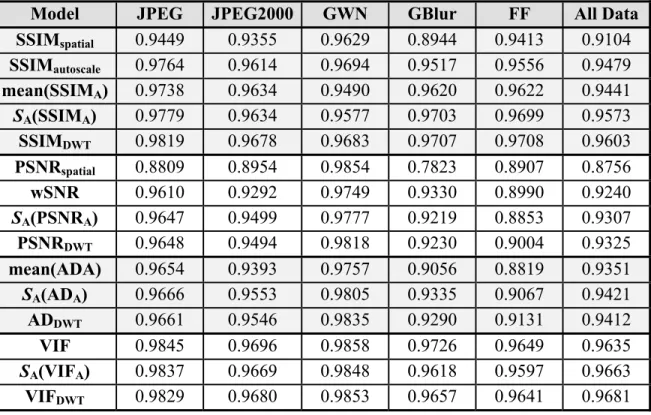
Table 3.1 LCC values after nonlinear regression for the LIVE image database. ...48

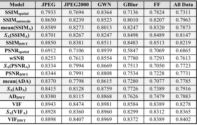
Table 3.2 SRCC values after nonlinear regression for the LIVE image database. ...48

Table 3.3 RMSE values after nonlinear regression for the LIVE image database. ...49

Table 3.4 KRCC values after nonlinear regression for the LIVE image database. ...49

Table 3.5 F-test results on the residual error predictions of different structure-based IQMS...51

Table 3.6 F-test results on the residual error predictions of various information-theoretic-based IQMS. ...51

Table 3.7 F-test results on the residual error predictions of various error-based IQMS...51

Table 3.8 Performance comparison of image quality assessment models for TID2008 image database (only images with distortion types of additive Gaussian noise, Gaussian blur, JPEG compression, JPEG2000 compression, JPEG transmission errors, and JPEG2000 transmission errors are included). ...53

Table 3.9 Performance comparison of image quality assessment models for H.264/AVC video compression using the LIVE video quality database. ...54

Table 5.1 Tabulation of significant encoding parameters for the H.264 JM18.3. ...96

Table 5.2 Comparison of the overall rates and distortions of H.264 compressed test sequences used in the experiment associated with investigating the relationship between distortion metrics SSE and SSEA. The encoded test sequences are all in CIF resolution with the frame rate of 30 Hz...98 Table 5.3 The relationship between pixel domain and wavelet domain metrics

(CIF, 30Hz). The distortion/quality metrics calculated for each 16×16 macroblock, and then metrics’ values averaged for each

frame over the whole sequence. ... 100 Table 5.4 The relationship between pixel domain and wavelet domain metrics

through different statistical methods for the frame number 25 of the sequence “foreman” (CIF, 30Hz). The distortion/quality

metrics calculated for each 16×16 macroblock. ... 100 Table 5.5 The relationship between pixel domain and wavelet domain metrics

through different statistical methods for the frame number 75 of the sequence “foreman” (CIF, 30Hz). The distortion/quality

metrics calculated for each 16×16 macroblock. ... 101 Table 5.6 The frequency of each inter coding mode used, for macroblocks in the P

slice, when encoding the first 100 frames of the sequence

“foreman”. ... 105 Table 5.7 Adapted mode decision Lagrange multiplier values obtained by the search

LIST OF FIGURES

Page Figure 1.1 Quality assessment approaches: (a) FR method, (b) NR method, (c) RR

method...8 Figure 1.2 A prototypical image quality assessment system based on error visibility.

(Adapted from (Wang and Bovik, 2006)) ...10 Figure 1.3 Diagram of the SSIM measurement system. (Adapted from (Wang et al.,

2004)) ...12 Figure 1.4 Multiscale structural similarity measurement. 2↓ denotes downsampling

by 2. (Adapted from (Wang, Simoncelli and Bovik, 2003)) ...14 Figure 1.5 SSIM-based video quality assessment system. (Adapted from (Wang, Lu

and Bovik, 2004)) ...15 Figure 1.6 VIF index system diagram. (Adapted from (Sheikh and Bovik, 2006)) ...17 Figure 2.1 Block diagram of the proposed discrete wavelet domain image quality

assessment framework. ...20 Figure 2.2 The wavelet subbands for a two-level decomposed image. ...24 Figure 2.3 (a) Original image; (b) Contrast map computed using Eq. (2.9). The

sample values of the contrast map are scaled between [0,255] for

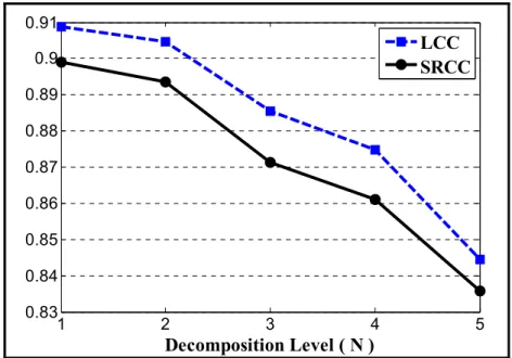
easy observation. ...26 Figure 2.4 LCC and SRCC between the MOS and mean SSIMA prediction values

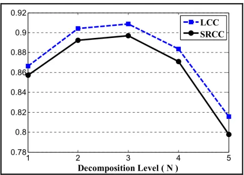
for various decomposition levels. ...28 Figure 2.5 LCC and SRCC between the MOS and VIFA prediction values for

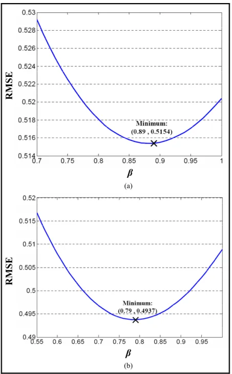
various decomposition levels. ...34 Figure 2.6 RMSE between the MOS and PSNRDWT prediction values for various β

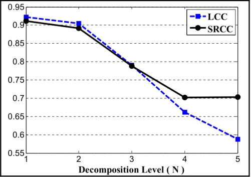
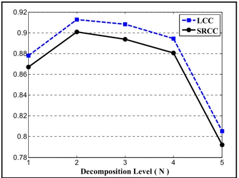
values at (a) N=2; (b) N=3. ...36 Figure 2.7 LCC and SRCC between the MOS and PSNRA prediction values for

various decomposition levels. ...38 Figure 2.8 LCC and SRCC between the MOS and mean ADA prediction values for

Figure 3.1 Comparison of the complexity of various quality metrics vs. H.264

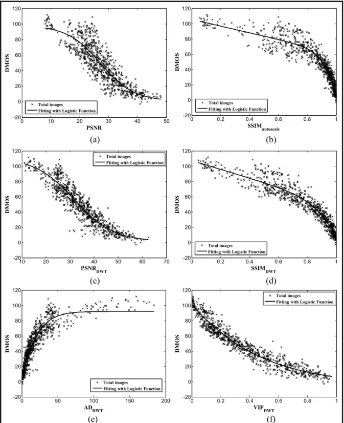
encoding complexity. ... 45 Figure 3.2 Scatter plots of DMOS versus model prediction for all distorted images

in the LIVE database. (a) PSNR; (b) SSIMautoscale; (c) PSNRDWT;

(d) SSIMDWT; (e) ADDWT; (f) VIFDWT. ... 52

Figure 4.1 Macroblock splitting process in H.264; (a) macroblock partitions; (b)

sub-macroblock partitions. ... 58 Figure 4.2 Macroblock mode decision program flow in a P-slice. ... 59 Figure 4.3 The RD cost computation process for a coding mode. (Adapted from

(Xin, Vetro and Sun, 2004)) ... 64 Figure 4.4 Block diagram of a hybrid video encoder including motion estimation

and mode decision blocks. (Adapted from (Xin, Vetro and Sun,

2004)) ... 69 Figure 4.5 The general framework of video encoding using SSIM-based approach.

(Adapted from (Huang et al., 2010)) ... 82 Figure 5.1 Scatter plot of SSE vs. SSEA for the frame number 25 of the sequence

“foreman” (CIF, 30Hz) coded with QP = 16. The distortion

metrics calculated for each 16×16 macroblock. ... 101 Figure 5.2 Scatter plot of SSE vs. SSEA for the frame number 25 of the sequence

“foreman” (CIF, 30Hz) coded with QP = 30. The distortion

metrics calculated for each 16×16 macroblock. ... 102 Figure 5.3 Scatter plot of SSE vs. SSEA for the frame number 25 of the sequence

“foreman” (CIF, 30Hz) coded with QP = 44. The distortion

metrics calculated for each 16×16 macroblock. ... 102 Figure 5.4 Scatter plot of SSE vs. SSEA for the frame number 75 of the sequence

“foreman” (CIF, 30Hz) coded with QP = 16. The distortion

metrics calculated for each 16×16 macroblock. ... 103 Figure 5.5 Scatter plot of SSE vs. SSEA for the frame number 75 of the sequence

“foreman” (CIF, 30Hz) coded with QP = 30. The distortion

metrics calculated for each 16×16 macroblock. ... 103 Figure 5.6 Scatter plot of SSE vs. SSEA for the frame number 75 of the sequence

“foreman” (CIF, 30Hz) coded with QP = 44. The distortion

Figure 5.7 Diagram of Lagrange multiplier generation for our proposed search

method...106 Figure 5.8 The 15 generated RD curves for 15 values of QP and 58 values of λp. The

test sequence is “container” and the number of frames encoded is 120. Each curve corresponds to a different value of QP and each

marker on the curve represents a specific Lagrange multiplier. ...110 Figure 5.9 The generated RD curves (from figure 5.8) and the envelope fitted to

them. Markers on the fitted curved have been represented by

squares...111 Figure 5.10 The rate-distortion curves for encoding 120 frames of sequence

“container”. ...112 Figure 5.11 The rate-distortion curves for encoding 120 frames of sequence

“foreman”. ...112 Figure 5.12 The rate-distortion curves for encoding 120 frames of sequence

“football”...113 Figure 5.13 The rate-distortion curves for encoding 30 frames of sequence

“container”. ...114 Figure 5.14 The rate-distortion curves for encoding 30 frames of sequence

“foreman”. ...114 Figure 5.15 The rate-distortion curves for encoding 30 frames of sequence

“football”...115 Figure 5.16 Adapted Lagrange multiplier values for various test sequences. ...117 Figure 5.17 The RD curves for encoding 120 frames of “container” when λMOTION ≠

λMODE. ...118

Figure 5.18 The RD curves for encoding 120 frames of “foreman” when λMOTION ≠

λMODE. ...118

Figure 5.19 The RD curves for encoding 120 frames of “football” when λMOTION ≠

λMODE. ...119

Figure 5.20 The RD curves for encoding 30 frames of “container” when λMOTION ≠

λMODE. ...119

Figure 5.21 The RD curves for encoding 30 frames of “foreman” when λMOTION ≠

Figure 5.22 The RD curves for encoding 30 frames of “football” when λMOTION ≠

λMODE. ... 120

Figure 5.23 The RD curves for encoding 120 frames of “akiyo” when λMOTION =

λMODE and using non-adapted λp. ... 121

Figure 5.24 The RD curves for encoding 120 frames of “hall” when λMOTION =

LIST OF ABREVIATIONS ACR Absolute Category Rating

AD Absolute Difference

AVC Advanced Video Coding

CABAC Context Adaptive Binary Arithmetic Coding CALM Context Adaptive Lagrange Multiplier CAVLC Context Adaptive Variable Length Coding CIF Common Intermediate Format

CSF Contrast Sensitivity Function

CW-SSIM Complex-Wavelet Structural SIMilarity dB Decibel

DCT Discrete Cosine Transform DPB Decoded Picture Buffer DWT Discrete Wavelet Transform

FF Fast Fading

FR Full-Reference

GBlur Gaussian Blurring

GSM Gaussian Scale Mixture GWN Gaussian White Noise

H.264 Digital video compression and encoding standard

HR High Rate

HVS Human Visual System IFC Information Fidelity Criterion

IPP Integrated Performance Primitives IQM Image Quality Metrics

JM Joint Model (H.264 reference software)

JVT Joint Video Team

KRCC Kendall Rank Correlation Coefficient LCC Linear Correlation Coefficient

MOS Mean Opinion Score

MPEG Moving Picture Experts Group MSE Mean Squared Errors

MSSIM Mean Structural SIMilarity

MV Motion Vector

NR No-Reference PSNR Peak Signal-to-Noise Ratio

QP Quantization Parameter

RF Random Field

RD Rate-Distortion

RDO Rate-Distortion Optimization RMSE Root Mean Square Error

RR Reduced-Reference

SRCC Spearman Rank Correlation Coefficient SAD Sum of Absolute Differences

SSD Sum of Squared Differences SSE Sum of Squared Errors SSIM Structural SIMilarity VDP Visible Difference Predictor VIF Visual Information Fidelity

INTRODUCTION Problem statement

Image/video coding and transmission systems may introduce some amount of distortion or artifacts in the original/reference signal. The commercial success of an image/video systems depends on their ability to deliver the users good image/video quality consistently. Therefore, image quality assessment plays an important role in the development and validation of various image and video applications, such as compression and enhancement.

The visual quality of an image (or video) is best assessed subjectively by human viewers. But the assessment of subjective quality is time consuming, expensive, and cannot be performed for real-time systems. Therefore, it is essential to define an objective criterion that can measure the difference between the original and the processed image/video signals. Ideally, such an objective measure should correlate well with the perceived difference between two image/video signals, and also varies linearly with the subjective quality.

Many image/video processing systems use mean squared errors (MSE), or equivalently peak signal-to-noise ratio (PSNR), as the objective quality assessment metric due to its simplicity. Because of the non-linear behavior of the human visual system, the PSNR values do not reflect accurately the perceived quality. Therefore, different objective models have arised for accurate visual quality assessment. An overview of the existing quality evaluation models reveals that the computational complexity of assessment techniques that accurately predict quality scores is very high. Owing to the high computational complexity of accurate methods, the PSNR (or MSE) is still used in many image/video processing applications. If we develop low-complexity quality metrics with high-accuracy, it is possible to use them in various real-time image and video processing tasks such as quality control and validation, and video compression with higher perceived quality.

Since the ultimate video quality is judged by human viewers, a well-designed video encoder should be ideally optimized in terms of human visual system perception. Generally speaking, the improvements of visual quality in the video encoding process mainly depend on the following two factors:

• The accuracy of the objective quality assessment models for video sequences.

• The approach to incorporate the objective models into the video encoding framework.

The first factor is addressed in the first part of our thesis, i.e. development of efficient visual quality metrics. Perceptual quality metrics can be adopted and integrated inside several different modules of a video encoder such as mode decision, motion estimation, quantization, and rate control and bit allocation (Su et al., 2012), (Ou, Huang and Chen, 2011), (Yu et al., 2005), (Yuan et al., 2006), (Hrarti et al., 2010).

The macroblock mode decision process is one of the most computationally intensive phases of the video encoding, which also contains within itself the motion estimation during inter-frame predictions. Therefore, it can directly affect the perceptual video quality. Due to its importance, we focus on the mode decision as a potential application of the visual quality metrics. In conventional video encoding mode decision process, sum of squared errors (SSE) is the commonly used metric for measuring the distortion for the ease of calculation. By developing low-complexity visual metrics, the SSE can be substituted with a more accurate metric that is well-correlated with the human evaluations in order to improve the video compression efficiency.

Research objectives

Based upon the shortcomings of the existing methods and the motivations stated in the previous section, we define the main goals of this thesis as follows:

• Develop a general low-complexity framework for full reference visual quality assessment of images (or video frames). This framework must include features for the computation of quality scores not only with lower computational complexity, but also with higher prediction accuracy.

• Create new computational methods for the advanced quality metrics such as SSIM (Wang et al., 2004) and VIF (Sheikh and Bovik, 2006) using the proposed framework. The new models must clearly inherit the mentioned features from the framework, i.e. lower computational complexity and higher prediction accuracy, compared to the original measures.

• Create error-based visual quality metrics for image/video quality assessment using the proposed framework.

• Validate the benefits of the developed quality assessment techniques against state-of-the-art methods by evaluating them on the different image and video quality databases.

• Incorporate the developed quality/distortion metrics, instead of the SSE, in the H.264/AVC mode decision process in order to optimize the video frames’ perceptual qualities in terms of the corresponding developed metric.

• Devise an appropriate approach to determine the new Lagrange multiplier values at each QP for the incorporated mode decision distortion metric.

• Implement our developed quality/distortion metric in the mode decision process of an H.264/AVC software, and obtain the rate-distortion curves to measure the performance improvement percentage by our proposed mode decision algorithm over the conventional SSE-based approach.

Organization of the thesis

This thesis consists of six main chapters and a conclusion chapter, which all follow this introduction chapter. In the chapter 1, we first introduce the concept of image/video quality assessment, and explain the need for the existence of objective visual quality evaluation models. Then, we explain two major categories in the visual quality evaluation. The

principles and important methods of each category are reviewed briefly, however the new category of top-down approaches are studied in more details due to its importance and also its application in the next chapters. At last, Chapter 1 ends with a discussion section which compares the most important methods against each other and gives the benefits of each of them.

In chapters 2 and 3, we present our proposed framework for calculating the visual quality scores with high prediction accuracy and low computational complexity. In the chapter 2, we describe the principles and theory of our framework, and in the chapter 3, we bring the simulation results of the framework using different image and video databases. Chapter 2 begins with clarifying the shortcomings of the existing quality assessment models and describing the motivations to find a solution approach to improve the performance of these models. After that, each part of our proposed wavelet domain framework is described in details. To show the practical usage of our framework to generate a new quality metric or improvement over an existing model, four different examples are brought afterwards. The first two examples are related to the methods in the category of top-down approaches, i.e. structural similarity approach and the information-theoretic approach. The next two examples are given on the traditional error-based quality models. The first error-based example is using the mean squared error of signals to propose a metric similar to PSNR but with much higher prediction accuracy. The second error-based example uses the absolute differences of the input signals as the distortion measure and benefits from the features of the framework to propose a totally new visual quality metric. It is notable that each of the four given examples is a new and independent visual quality metric on its own.

Chapter 3 shows the simulation results of our framework and the metrics explained in the chapter 2. At first, the computational complexity of different algorithms, working based on the framework, is discussed theoretically and numerically. Then, the prediction accuracy of our metrics is verified using different statistical performance measures. Our tests are performed on three well-known databases: two different image quality databases and a video

quality database. This chapter will finally present concluding remarks on the visual quality metrics based on the simulated results.

In the chapter 4, we review different approaches for macroblock mode decision in video encoding. Inter prediction and various macroblock partitions in H.264/AVC are introduced in the beginning. Then, the Lagrange multiplier estimation is explained as a solution for performing rate distortion optimized mode decision in H.264. After describing the conventional process of encoding a macroblock, important adaptive methods are reviewed to estimate the Lagrange multiplier per video frame. Finally, we study different HVS-based techniques for the Lagrange multiplier calculation. This review provides insights for efficiently using our proposed metrics for mode decision.

Chapter 5 describes our perceptual-based approach for rate-distortion optimized (RDO) mode decision in H.264 Baseline coding. This chapter starts by explaining the pros and cons of existing methods and our motivations behind proposing a new technique for mode decision. Then, the details are given on the proposed approach for the perceptual mode selection. In order to find the best way of determining the corresponding Lagrange multiplier in our method, we analyze the relationships of macroblock distortions in different domains theoretically and empirically. In the next step, we present our proposed search method for the determination of the Lagrange multiplier at each QP. After determining the Lagrange multipliers, the simulated rate-distortion (RD) curves are shown for different types of sequences. The RD curves are simulated for both cases of applying adapted and non-adapted Lagrange multipliers. Finally in the concluding section, the potential gains from our improved method are discussed, along with some suggestions for the future research.

In the chapter 6, we list the contributions of our research on the visual quality metrics and H.264 coding mode decision. The last chapter, the conclusion, summarizes the important research results in our thesis and offers the final concluding remarks.

CHAPTER 1

DIGITAL IMAGE AND VIDEO QUALITY ASSESSMENT MODELS AND METRICS

In this chapter, we first explain the general concept of image/video quality assessment. Then, we classify objective visual quality measures, and introduce the main methods of image/video quality evaluation in a nutshell. In the next chapter, we give details of our proposed framework for accurate quality assessment.

1.1 Introduction

As mentioned in the problem statement, an objective criterion is required to measure the level of artifacts and predict the perceptual quality in an image/video processing systems. Objective quality models are usually classified based on the availability of the original image/video signal, which is considered to be of high quality (generally not processed). Generally, quality assessment methods can be classified as full reference (FR) methods, reduced-reference (RR) methods, and no-reference (NR) methods (Wang and Bovik, 2006), as shown in figure 1.1.

FR metrics usually compute the visual quality by comparing every pixel/sample in the distorted image to its corresponding pixel/sample in the original image signal. NR metrics assess the quality of a distorted signal without any reference to the original signal. The NR metrics are usually designed to be application-specific, that is, they directly measure the types of artifacts created by the specific image distortion processes, e.g., blocking by block-based compression and ringing by wavelet-block-based compression. RR metrics extract some features of both original and distorted signals, and then compare them to give a quality score. They are used when the whole original image/video signal is not available, e.g. in a transmission with a limited bandwidth. In this thesis, we specifically focus on studying and developing the FR quality metrics because they currently lead to higher accuracy.

Figure 1.1 Quality assessment approaches: (a) FR method, (b) NR method, (c) RR method.

The mean squared error (MSE) is the most traditional way of measuring the signal fidelity. The goal of a signal fidelity measure is to compare two signals by providing a quantitative score that describes the degree of similarity/ fidelity or, conversely, the level of error/distortion between them (Wang and Bovik, 2009). If we suppose that

{

x i_i 1, 2, ,N

}

= =

X _ and Y=

{

y i_i =1, 2, ,_ N

}

are two finite-length, discrete signals (e.g., visual images), the MSE between the two signals is defined as in Eq. (1.1).

(

)

(

)

2 1 1 MSE , N _{i i} i x y N ₌ =



− X Y (1.1)

where N is the number of signal samples (pixels, if the signals are images), and xi and yi are

the values of the ith samples in X and Y respectively. If one of the signals is considered as an original signal (of acceptable quality), and the other as the distorted version of it whose quality is being evaluated, then the MSE can also be regarded as a measure of signal quality.

In the literature of image/video processing, MSE is usually converted into a peak signal-to-noise ratio (PSNR) measure. The PSNR is more useful than the MSE for comparing images having different dynamic ranges (Wang and Bovik, 2009). The MSE (or equivalently PSNR) is the most widely used objective quality metric in image/video applications. The reason is that the MSE is simple and has a clear physical meaning. It is naturally representative of the error signal energy. In addition, the MSE is an excellent objective metric in the context of optimization and statistical estimation framework. In spite of many favorable properties of MSE, it does not correlate well with the perceived visual quality due to non-linear behavior of the human visual system (HVS).

In (Huynh-Thu and Ghanbari, 2008), the authors have set experiments to investigate where PSNR can or cannot be used as a reliable quality metric. They encoded input sequences at various bit-rates (24-800 kbit/s) with H.264 coding format, and then the decoded sequences were assessed subjectively using ACR international standard method (ITU-T Recommendation P.910). They have found that for a specified content (sequence), the PSNR always monotonically increases with subjective quality as the bit rate increases. Therefore, the PSNR can be used as a performance metric for codec optimization as it correlates highly with subjective quality when the content is fixed. In spite of the existence of monotonic relationship between the PSNR and subjective quality separately per content, it does not exist anymore across different contents. This means different video contents with the same PSNR may have in fact a very different perceptual quality. The PSNR is therefore unreliable as an objective metric for predicting subjective quality. Briefly, the PSNR is not a reliable measure of quality across various video contents, but it is reliable within the content itself (Huynh-Thu and Ghanbari, 2008). Due to deficiencies of PSNR in providing accurate quality predictions, other quality assessment models have been developed by researchers.

Generally speaking, the full reference quality assessment of image and video signals involves two categories of approach: bottom-up and top-down (Wang and Bovik, 2006). In the next sections, we give a brief overview of each approach and introduce main methods in either of them.

1.2 Bottom-up approaches for visual quality assessment

In the bottom-up approaches, perceptual quality scores are best estimated by quantifying the visibility of errors. In order to quantize errors according to the HVS features, techniques in this category try to model the functional properties of different stages of the HVS as characterized by both psychophysical and physiological experiments. This is usually accomplished in several stages of preprocessing, frequency analysis, contrast sensitivity, luminance masking, contrast masking, and error pooling (Wang and Bovik, 2006), (Bovik, 2009), as shown in figure 1.2.

. . . _{. . .}

Figure 1.2 A prototypical image quality assessment system based on error visibility. (Adapted from (Wang and Bovik, 2006))

Most of HVS-based quality assessment techniques are multi-channel models, in which each band of spatial frequencies is dealt with by an independent channel. Several important methods of this category have been briefly explained in the annex I.

The bottom-up approaches have several important limitations, which are discussed in (Wang and Bovik, 2006), (Wang et al., 2004). In particular, the HVS is a complex and highly nonlinear system, but most models of early vision are based on linear or quasi-linear operators that have been characterized using restricted and simplistic stimuli. The limited numbers of simple-stimulus experiments are not enough to build a prediction model for perceptual quality that has complex structures. Furthermore, prior information regarding the image content, or attention and fixation likely affect the evaluation of visual quality. These effects are not understood, and are usually ignored by image quality models.

1.3 Top-down approaches for visual quality assessment

The second category of full reference quality assessment includes top-down approaches. In the top-down techniques, the overall functionality of the HVS is considered as a black box, and the input/output relationship is of interest. Thus, top-down approaches do not require any calibration parameters from the HVS or viewing configuration. Two main strategies applied in this category are the structural similarity approach and the information-theoretic approach.

1.3.1 Structural similarity approach

The principal idea underlying the structural similarity approach is that the HVS is highly adapted to extract structural information from visual scenes, and therefore, a measurement of structural similarity (or distortion) should provide a good approximation of the perceptual image quality. In fact, this philosophy considers image degradations as perceived changes in structural information variation. In contrast to error sensitivity concept which is a bottom-up approach and simulating early-stage components in the HVS, structural similarity paradigm is a top-down approach that is mimicking the hypothesized functionality of the overall HVS.

Perhaps the most important method of the structural approach is the Structural SIMilarity (SSIM) index (Wang et al., 2004), which gives an accurate score with acceptable computational complexity compared with other quality metrics (Sheikh, Sabir and Bovik, 2006). SSIM has attracted a great deal of attention in recent years, and has been considered for a wide range of applications. The SSIM is a space domain implementation of the structural similarity idea. In this method, each image can be represented as a vector whose entries are the gray scales of the pixels in the image. The SSIM separates the task of similarity measurement into three comparisons: luminance, contrast and structure. As we know, the luminance of the surface of an object that is imaged or observed is the product of the illumination and the reflectance. The major impacts of illumination changes in an image are variations in the average local luminance and contrast values, but the structures of the objects in the scene are independent of the illumination. Consequently, it is desirable to

separate measurements of luminance and contrast distortions from the other structural distortions that may afflict the image. The diagram of SSIM quality assessment is shown in figure 1.3.

Figure 1.3 Diagram of the SSIM measurement system. (Adapted from (Wang et al., 2004))

Suppose that x and y are local image patches taken from the same location of two images that are being compared. As mentioned, the local SSIM index measures the similarities of three elements of the image patches: the luminance similarity l(x,y) of the local patch (brightness values), the contrast similarity c(x,y) of the local patch, and the structural similarity s(x,y) of the local patch. These local similarities are expressed using simple, easily computed statistics, and combined together to form local SSIM:

( )

1 2 3 2 2 2 2 1 2 3 2 2 SSIM , ( , ) ( , ) ( , ) x y x y xy x y x y x y c c c l c s c c c μ μ σ σ σ μ μ σ σ σ σ  ₊   ₊   ₊  = ⋅ ⋅ =_  _{ }⋅  _{ }⋅ _ + + + + +       x y x y x y x y (1.2)

where μx and μy are (respectively) the local sample means of x and y, σx and σy are the local

sample standard deviations of x and y, and σxy is the sample cross correlation of x and y after

removing their means. The items c1, c2, and c3 are small positive constants that stabilize each

term, so that near-zero sample means, variances, or correlations do not lead to numerical instability. In (Wang et al., 2004), robust quality assessment results are obtained using Eq. (1.2) by setting c3 to c2/2. The SSIM index satisfies the following properties:

• Boundedness: SSIM(x,y) ≤ 1

• Unique maximum: SSIM(x,y) = 1 if and only if x = y

The SSIM index is computed locally (on image blocks or patches). The main reason is that image statistical features are usually highly spatially non-stationary. The local statistics μx, σx

and σxy as well as the SSIM index, are computed within a local window that moves

pixel-by-pixel from the top-left to the bottom-right corner of the image. In (Wang et al., 2004), an 11×11 circular-symmetric Gaussian weighting function (normalized to unit sum ) with standard deviation of 1.5 pixels is employed. This choice of window prevents exhibition of blocking artifacts in the SSIM index map and the quality maps show a locally isotropic property. The overall SSIM score of the entire image is then computed by simply averaging the SSIM map:

1 1 MSSIM( , ) M SSIM( , ) j M ₌ =



j j X Y x y _(1.3)

where X and Y are the reference and the distorted images, respectively; xj and yj are the

image contents at the jth local window; and M is the number of local windows of the image. The MSSIM is only calculated based on the luminance component of images.

There have been attempts made to improve the SSIM index assessment accuracy. Multi-scale SSIM method (Wang, Simoncelli and Bovik, 2003) for quality assessment provides more flexibility than single-scale SSIM index in incorporating image details at several different resolutions. In this method, an image synthesis-based approach is used to calibrate the parameters that weight the relative importance between different scales. The system diagram for multi-scale SSIM is shown in figure 1.4. The multi-scale SSIM iteratively applies low pass filtering and downsampling up to five different resolutions. The original image is indexed as Scale 1, and the highest scale as Scale M (i.e. 5), which is obtained after (M−1) iterations. At the jth scale, only the contrast comparison ( , )c x y and the structure comparison _j

) , ( yx j

denoted as l x y . The overall SSIM evaluation is obtained by combining the measurement _M( , ) at different scales using:

M M multi-scale M 1 SSIM ( , ) [ ( , )] . [ ( , )] [ ( , )]j j j j j l α c β s λ = =

∏

x y x y x y x y _(1.4)

The exponents αM, βj, and λj are used to adjust the relative importance of different

components. To simplify parameter selection, we let αj = βj = λj for all j’s. In addition, the

cross-scale settings are normalized such that M_{j 1λj} 1

= =



. The resulting parameters obtained in (Wang, Simoncelli and Bovik, 2003) according to experiments are: β1 = λ1 = 0.0448, β2 =

λ2 = 0.2856, β3 = λ3 = 0.3001, β4 = λ4 = 0.2363, and α5 = β5 = λ5 = 0.1333.

Figure 1.4 Multiscale structural similarity measurement. 2↓ denotes downsampling by 2. (Adapted from (Wang, Simoncelli and Bovik, 2003))

In (Rouse and Hemami, 2008), the authors investigate ways to simplify SSIM in the pixel domain. They study the contribution of each SSIM component in evaluation of common image artifacts. It is finally concluded that by ignoring the mean component in Eq. (1.2) and setting the local average patch values to 128, the linear correlation coefficient is decreased just 1% from the complete computation of the SSIM. The authors in (Yang, Gao and Po, 2008) propose to compute SSIM using subbands at different levels in the discrete wavelet domain. Five-level decomposition using the Daubechies 9/7 wavelet is applied to both the original and the distorted images, and then SSIMs are computed between corresponding subbands. Finally, the similarity score is obtained by the weighted sum of all mean SSIMs.

To determine the weights, a large number of experiments have been performed to measure the sensitivity of the human eye to different frequency bands.

CW-SSIM, which is presented in (Wang and Simoncelli, 2005) and (Sampat et al., 2009), benefits from a complex version of 6-scale, 16-orientation steerable pyramid decomposition characteristics to propose a metric resistant to small geometrical distortions. CW-SSIM is simultaneously insensitive to luminance change, contrast change and spatial translation. The CW-SSIM does not rely on any registration or intensity normalization pre-processing, and just exploits the fact that small translations, scalings, and rotations lead to consistent, describable phase changes in the complex wavelet domain. Yet this method works only when the amount of translation, scaling and rotation is small (compared to the wavelet filter size). In fact, the CW-SSIM is equivalent to applying the spatial domain SSIM index to the magnitudes of the coefficients, where the luminance comparison part is not included since the coefficients are zero-mean (due to the bandpass nature of the wavelet filters). Briefly, the CW-SSIM metric works upon two facts. First, the structural information of local image features is mainly contained in the relative phase patterns of the wavelet coefficients. Second, consistent phase shift of all coefficients does not change the structure of the local image features.

Figure 1.5 SSIM-based video quality assessment system. (Adapted from (Wang, Lu and Bovik, 2004))

For video quality assessment using structural similarity, SSIM Index is employed as a single measure for various types of distortions. The quality of the distorted video is measured in

three levels as shown in figure 1.5: the local region level, the frame level, and the sequence level (Wang, Lu and Bovik, 2004). Further details about the quality score computation procedure can be found in (Wang, Lu and Bovik, 2004).

For our video quality assessment in next chapters, the image quality metric is applied frame-by-frame on the luminance component of the video, and the overall video quality index is computed as the average of the frame level quality scores. It is known that compression systems, like H.264, produce fairly uniform distortions (or quality) in the video, both spatially and temporally (Seshadrinathan et al., 2010a). Therefore, we suppose that averaging the frames quality scores is an acceptable pooling strategy for assessment of H.264 compression performance.

1.3.2 Information-theoretic approach

In the information-theoretic approach, visual quality assessment is viewed as an information fidelity problem. Methods in this category attempt to relate visual quality to the amount of information that is shared between the images being compared. Shared information is quantified using the mutual information that is a statistical measure of information fidelity. An information fidelity criterion (IFC) for image quality measurement is presented in (Sheikh, Bovik and De Veciana, 2005), which works based on natural scene statistics. In the IFC, the image source is modeled using a Gaussian scale mixture (GSM), while the image distortion process is modeled as an error-prone communication channel. As mentioned, the information shared between the images being compared is quantified using the mutual information. Another information-theoretic quality metric is the visual information fidelity (VIF) index (Sheikh and Bovik, 2006). This index follows the same procedure as the IFC, except that, in the VIF, both the image distortion process and the visual perception process are modeled as error-prone communication channels. The VIF index is one of the most accurate image quality metric, especially when dealing with large image databases (Sheikh, Sabir and Bovik, 2006) and (Wang and Li, 2011). The system diagram of VIF Index is illustrated in figure 1.6.

Figure 1.6 VIF index system diagram. (Adapted from (Sheikh and Bovik, 2006))

In spite of high level of prediction accuracy of VIF, this index has not been given as much consideration as the SSIM index in a variety of applications. This is probably because of its high computational complexity (6.5 times the computation time of the SSIM, index according to (Sheikh and Bovik, 2006)). Most of the complexity in the VIF index comes from over-complete steerable pyramid decomposition, in which the neighboring coefficients from the same subband are linearly correlated. Consequently, the vector Gaussian scale mixture GSM is applied for accurate quality prediction. The decomposed coefficients in each subband are partitioned into non-overlapping blocks of coefficients. Since the blocks do not overlap, each block is assumed to be independent of others, and modeled as a vector. In the next chapter, we propose a low-complexity version of VIF index.

1.4 Discussion

In (Sheikh, Sabir and Bovik, 2006), several prominent full reference image quality measures, from both bottom-up and top-down approaches, were statistically evaluated across a wide variety distortion types. It is reported that VIF index exhibits superior performance relative to all prior methods for image quality assessment, however the performance of the VIF index and the SSIM index are close across a broad diversity of representative image distortion types. As mentioned before, it is more difficult to compute VIF index than SSIM.

Top-down methods are new and fast-evolving compared with bottom-up approaches. Generally, there are some advantages of using top-down methods against bottom-up approaches. Top-down approaches are more accurate and often lead to simpler implantations. Moreover, top-down approaches are more mathematically tractable. For example, the SSIM

index is differentiable, which is useful in gradient-based optimization routines. Both VIF index and SSIM index are bounded between zero and one, while the quality assessment methods belonging to bottom-up approaches do not usually have any specific upper and lower bounds.

CHAPTER 2

THE PROPOSED LOW-COMPLEXITY DISCRETE WAVELET TRANSFORM FRAMEWORK FOR FULL REFERENCE IMAGE QUALITY ASSESSMENT 2.1 Motivation

In this chapter, we propose a novel general framework to calculate image quality metrics (IQM) in the discrete wavelet domain. The proposed framework can be applied to both top-down and error-based (bottom-up) approaches, as explained in subsequent sections. This framework can be applied to map-based metrics, which generate quality (or distortion) maps such as the SSIM map and the absolute difference (AD) map, or to non map-based ones, which give a final score such as the PSNR and the VIF index. We also show that, for these metrics, the framework leads to improved accuracy and reduced complexity compared to the original metrics.

We developed the new framework mainly because of the following shortcomings of the current methods. First, the computational complexity of assessment techniques that accurately predict quality scores is very high. If we develop high-accuracy low complexity quality metrics, it is possible to use them in real-time image/video processing applications such as motion estimation and video encoding rate control (Yasakethu et al., 2008), can be solved more efficiently if an accurate low complexity quality metric is used. Second, the bottom-up approach reviewed (Teo and Heeger, 1994),(Chandler and Hemami, 2007) specifies that those techniques apply the multi-resolution transform, decomposing the input image into large numbers of resolutions (five or more). As the HVS is a complex system that is not completely known to us, combining the various bands into the final metric is difficult. In similar top-down methods, such as multi-scale and multi-level SSIMs (Wang, Simoncelli and Bovik, 2003), (Yang, Gao and Po, 2008), determining the sensitivity of the HVS to different scales or subbands requires many experiments. Our new approach does not require such heavy experimentation to determine parameters. Third, top-down methods, like SSIM, gather local statistics within a square sliding window, and the computed statistics of image

blocks in the wavelet domain are more accurate. Fourth, a large number of decomposition levels, as in (Yang, Gao and Po, 2008), would make the size of the approximation subband very small, so it would no longer be able to help in extracting image statistics effectively. In contrast, the approximation subband contains the main image content, and we have observed that this subband has a major impact on improving quality prediction accuracy. Fifth, previous SSIM methods use the mean of the quality map to give the overall image quality score. However, distortions in various image areas have different impacts on the HVS. In our framework, we introduce a contrast map in the wavelet domain for pooling quality maps.

In the rest of this chapter, we first describe our proposed general framework for image quality assessment. Then, we explain how the proposed framework is used to calculate the currently well-known objective quality metrics.

2.2 The proposed discrete wavelet domain image quality assessment framework

N A X N A Y

Figure 2.1 Block diagram of the proposed discrete wavelet domain image quality assessment framework.

In this section, we describe a DWT-based framework for computing a general purpose FR image quality metric (IQM). The block diagram of the proposed framework is shown in figure 2.1. The dashed lines in this figure display the parts that may be omitted based on whether or not it is a map-based metric. Let X and Y denote the reference and distorted

images respectively. The procedure for calculating the proposed version of IQM is set out and explained in the following steps.

Step 1. We perform N-level DWT on both the reference and the distorted images based on the Haar wavelet filter. With N-level decomposition, the approximation subbands XA_N and

YA_N, as well as a number of detail subbands, are obtained.

The Haar wavelet is the oldest and the simplest wavelet. Haar wavelet has very interesting properties including symmetry, orthogonality, biorthogonality, and compact support (Daubechies, 1992). Since the Haar wavelet is orthogonal, the frequency components of input signal can be analyzed. The length of low-pass and high-pass filters for the Haar wavelet is 2. The Haar decomposition low-pass filter Lo_D and the decomposition high-pass filter Hi_D are defined as Lo D=

( )

1 2

[ ]

1 1 and Hi D=

( )

1 2

[

-1 1

]

, respectively (Daubechies, 1992). For discrete 2-D (two dimensional) wavelet decomposition, these filters are applied to rows, and then to columns of the image signal. There is no need for multiplications in Haar transform. It requires only additions and a final scaling, so the computation time is very short. In fact, we just perform a simple averaging of the original signal to obtain the approximation subband. For example, for a single decomposition level, if the pixel intensities in a 2×2 window are assumed to be P1, P2, P3, and P4, the resulting

approximation coefficient would be 0.5(P1+P2+P3+P4). Since a kind of averaging process is

performed within the HVS when looking at the visual scenes, the characteristics of the Haar wavelet helps to emulate this feature of HVS for quality assessment.

The Haar wavelet has been used previously in some quality assessment and compression methods (Bolin and Meyer, 1999),(Lai and Kuo, 2000). For our framework, we chose the Haar filter for its simplicity and good performance. The Haar wavelet has very low computational complexity compared to other wavelets. In addition, based on our simulations, it provides more accurate quality scores than other wavelet bases. The reason for this is that symmetric Haar filters have a generalized linear phase, so the perceptual image structures can

be preserved. Also, Haar filters can avoid over-filtering the image, owing to their short filter length.

The number of levels (N) selected for structural or information-theoretic strategies, such as SSIM or VIF, is equal to one. The reason for this is that, for more than one level of decomposition, the resolution of the approximation subband is reduced exponentially and it becomes very small. Consequently, a large number of important image structures or information will be lost in that subband. But, for error-based approaches, like PSNR or absolute difference (AD), we can formulate the required decomposition levels N as follows: when an image is viewed at distance d from a display of height h, we have (Wang, Ostermann and Zhang, 2002):

d _{(cycles/degree)} 180 h s

f_θ = π f (2.1)

where fθ is the angular frequency that has a cycle/degree (cpd) unit; and fs denotes the spatial

frequency. For an image of height H, the Nyquist theorem results in Eq. (2.2):

( )

H (cycles/picture height)

2 s max

f = (2.2)

It is known that the HVS has a peak response for frequencies at about 2-4 cpd. We chose fθ =

3. If the image is assessed at a viewing distance of d₌kh, using Eq. (2.1) and Eq. (2.2), we deduce Eq. (2.3): 360 360 3 344 H (d/h) 3.14 f k k θ π × ≥ = ≈ × (2.3)

So, the effective size of an image for human eye assessment should be around (344/k). Accordingly, the minimum size of the approximation subband after N-level decomposition should be approximately equal to (344/k). For an image of size H×W, N is calculated as follows (considering that N must be non negative):

(

)

2 N min(H, W) 344 min(H, W) N round log 2 k 344 /k    ≈  = _ _ __     (2.4)

(

)

2 min(H, W) N 0 N max 0, round log

344 / k       ≥  = _ _ _ __       (2.5)

Step 2. We calculate the quality map (or score) by applying IQM between the approximation subbands of XA_N and YA_N, and call it the approximation quality map (or score), IQMA.

Examples of IQM computations applied to various quality metrics, such as SSIM and VIF, will be presented in the next section.

Step 3. An estimate of the image edges is formed for each image using an aggregate of detail subbands. If we apply the N-level DWT to the images, the edge map (estimate) of image X is defined as: N E E,L L 1 ( , ) ( , ) = =



X m n X m n (2.6)

where XE is the edge map of X; and XE,L is the image edge map at decomposition level L,

computed as defined in Eq. (2.7). In Eq. (2.7), XH_L, XV_L, and XD_L denote the horizontal,

vertical, and diagonal detail subbands obtained at the decomposition level L for image X respectively. XH_L,A_N-L, XV_L,A_N-L, and XD_L,A_N-L are the wavelet packet approximation subbands

obtained by applying an (N−L)-level DWT on XH_L, XV_L, and XD_L respectively. The

parameters µ, λ, and ψ are constant. As the HVS is more sensitive to the horizontal and vertical subbands and less sensitive to the diagonal one, greater weight is given to the horizontal and vertical subbands. We arbitrarily propose µ = λ = 4.5ψ in this paper, which results in µ = λ = 0.45 and ψ = 0.10 to satisfy Eq. (2.8).

(

) (

) (

)

(

) (

) (

)

L L L L N-L L N-L L N-L 2 2 2 H V D E,L 2 2 2 H ,A V ,A D ,A ( , ) ( , ) ( , ) if L N ( , ) ( , ) ( , ) ( , ) if L < N μ λ ψ μ λ ψ  ⋅ + + =  =   _{⋅ + +}  X X X X X X X m n m n m n m n m n m n m n (2.7) 1 μ λ ψ+ + = (2.8) 1 1 H ,A X 1 1 H ,H X 1 1 H ,V X X_{H ,D1 1} 1 1 D ,D X 1 1 D ,V X 1 1 D ,A X X_{D ,H1 1} 1 1 V ,A X X_{V ,H1 1} 1 1 V ,V X X_{V ,D1 1} 2 H X 2 A X 2 V X X_D2

Figure 2.2 The wavelet subbands for a two-level decomposed image.

The edge map of Y is defined in a similar way for X. As an example, Figure 2.2 depicts the subbands of image X for N=2. The subbands involved in computing the edge map are shown in color in this figure. It is notable that the edge map is intended to be an estimate of image edges. Thus, the most informative subbands are used in forming the edge map, rather than considering all of them. It is notable that edge maps of different subbands are of the same size, so they can be combined together without any problem.

In our method, we use only 3N edge bands. If we considered all the bands in our edge map, we would have to use 4N−1 bands. When N is greater than or equal to 2, the value 4N−1 is much greater than 3N. Thus, our proposed edge map helps save computation effort. According to our simulations, considering all the image subbands in calculating the edge map does not have a significant impact on increasing prediction accuracy. It is notable that the edge maps only reflect the fine-edge structures of images.

Step 4. We apply IQM between the edge maps XE and YE. The resulting quality map (or

score) is called the edge quality map (or score), IQME.

Step 5. Some metrics, like AD or SSIM, generate an intermediate quality map which should be pooled to reach the final score. In this step, we form a contrast map function for pooling the approximation and edge quality maps. It is well known that the HVS is more sensitive to areas near the edges (Wang and Bovik, 2006). Therefore, the pixels in the quality map near the edges should be given more importance. At the same time, energy (or high-variance) image regions are likely to contain more information to attract the HVS (Wang and Shang, 2006). Thus, the pixels of a quality map in high-energy regions must also receive higher weights (more importance). Based on these facts, we can combine our edge map with the computed variance to form a contrast map function. The contrast map is computed within a local Gaussian square window, which moves (pixel by pixel) over the entire edge maps XE

and YE. As in (Wang et al., 2004), we define a Gaussian sliding window

{

w k_k 1, 2, , K

}

= =

W  with a standard deviation of 1.5 samples, normalized to unit sum.

Here, we set the number of coefficients K to 16, that is, a 4×4 window. This window size is not too large and can provide accurate local statistics. The contrast map is defined as follows:

N N E A 2 2 0.15 E A ( , ) ( _{x x} ) Contrast x x _{= μ σ (2.9)} N N N A A K 2 2 A , 1 ( ) k k k x w x x σ μ = =



− (2.10) N E A N K K E, A , 1 1 , k k k k k k x w x x w x μ μ = = =



=



(2.11)

where xE and xAN denote image patches of XE and XAN within the sliding window. It is

notable that the contrast map merely exploits the original image statistics to form the weighted function for quality map pooling and statistics of the distorted image are not used.

The reason is that structures of the image may change due to distortion, so the statistics of distorted image are not very accurate.

Figure 2.3 (a) Original image; (b) Contrast map computed using Eq. (2.9). The sample values of the contrast map are scaled between [0,255] for easy observation.

Figure 2.3(b) demonstrates the resized contrast map obtained by Eq. (2.9) for a typical image in figure 2.3(a). As can be seen in figure 2.3, the contrast map nicely shows the edges and important image structures to the HVS. Brighter (higher) sample values in the contrast map indicate image structures that are more important to the HVS and play an important role in judging image quality.

Step 6. For map-based metrics, the contrast map in Eq. (2.9) is used for weighted pooling of the approximation quality map IQMA and the edge quality map IQME.

N N N N M E, A , A A , A , 1 M E, A , 1 ( , ) IQM ( , ) ( , ) j j j j j A j j j Contrast S Contrast = = ⋅ =





x x x y x x (2.12)