Application of nodal equivalence theory to the neutronic analysis of PWRS

APPLICATION OF NODAL EQUIVALENCE THEORY TO THE NEUTRONIC ANALYSIS OF PWRS

by

Christopher Lloyd Hoxie

B. S., University of Florida (1975)

SUBMITTED IN PARTIAL FULFILLMENT OF THE REQUIREMENTS FOR THE

DEGREE OF

DOCTOR OF PHILOSOPHY AT THE

MASSACHUSETTS INSTITUTE OF TECHNOLOGY JUNE 1982

MASSACHUSETTS INSTITUTE OF TECHNOLOGY 1982

Signature of Author .

Department of Nuclear Engineering June 1982 Certified by . . . -. . ... .an.. .Henry 4 Thesis Supervisor Accepted by .

pan F. Henry Chairman, Department Graduate Committee

Archives

OF TiUCHNLOGY

AUG

1 6

1982

APPLICATION OF NODAL EQUIVALENCE THEORY TO

THE NEUTRONIC ANALYSIS OF PWRs

by

Christopher Lloyd Hoxie

Submitted to the Department of Nuclear Engineering on May 21, 1982 in partial fulfillment of the requirements for the Degree of Doctor of

Philosophy in the field of Nuclear Engineering ABSTRACT

The objective of this research is to apply the analytic nodal method and nodal equivalence theory as embodied in the nodal code,

QUANDRY, to the neutronic analysis of pressurized water reactors (PWRs). This includes applying QUANDRY to the calculation of normalized

assembly power distributions for PWRs and devising, implementing and testing a heterogeneous PWR flux reconstruction scheme for QUANDRY.

In this research equivalence parameters are derived from hetero-geneous assembly calculations. These parameters are then employed in QUANDRY calculations. For realistic PWR problems it was found that this procedure leads to maximum errors in normalized assembly power densities of about 2%. The use of assembly equivalence param-eters did not lead to any consistent improvement in the accuracy of calculated xower distributions as campared to conventional flux-weighting methods of spatial hc•nogenization. However, it was found that the use of assembly equivalence parameters leads to more accurate prediction (less than 2% error) of the heterogeneous surface fluxes than the flux-weighting methods (about 7% error). This is an impor-tant result since such surface fluxes are input into heterogeneous flux reconstruction schemes.

A method of heterogeneous flux reconstruction is introduced called the form function method. This technique uses node-averaged informa-tion from the nodal code QUANDRY to construct an approximate form function which is then multiplied into a detailed flux shape frcm an inexpensive assembly criticality calculation to yield the recon-structed global heterogeneous flux within an assembly. For nodes near the steel baffle at the edge of a PWR core, extended assembly criticality calculations are employed in which the baffle and water reflector are included.

Use of the form function method on realistic PWR cores leads to maximum errors in the pointwise reconstructed flux of 3.5% for

assem-blies in the interior of the PWR core. For points in the core adjacent to the steel baffle, the maximum error may be 5.9%. Pin powers are calculated to within 4% maximum error.

TABLE OF CONTENTS Page Abs tract Acknowledgments List of Figures List of Tables Chapter 1. INTRODUCTION 1.1 Overview

1.2 Historical Review of Nodal Method Developments

1.3 A Reveiw of Spatial Homogenization of PWR Assemblies

1.4 Reconstruction of Heterogeneous PWR Fluxes From Nodal Calculations 1.5 Summary and Objective

Chapter 2

2.1 2.2

. A REVIEW OF THE ANALYTIC NODAL

METHOD AND NODAL EQUIVALENCE THEORY

Introduction

The QUANDRY Equations 2.2.1 Introduction

2.2.2 The Nodal Balance Equation 2.2.3 Differential Equation for the

One-Dimensional Homogeneous Fluxes

2.2.4 Equations for Homogeneous Surface Fluxes At a Nodal Interface u

xii xiii xxvi 1-1 1-1 1-3 1-7 1-12 1-20 2-1 2-1 2-3 2-3 2-4 2-8 2-17

2.3 Nodal Equivalence Theory

2.4 Homogeneous Cross Sections and Discontinuity Factors Based on

Heterogeneous Assembly Calculations 2.4.1 Introduction

2.4.2 The Heterogeneous Assembly Flux 2.4.3 Assembly Homogenized Cross

Sections and Diffusion Coefficients

2.4.4 Assembly Discontinuity Factors 2.4.5 Heterogeneous Extended

Assembly Calculations

2.4.6 Unity Discontinuity Factors

Chapter 3. APPLICATION OF NODAL EQUIVALENCE THEORY TO PWR BENCHMARK PROBLEMS 3.1 Introduction

3.2 Description of PWR Benchmark Problems 3.3 Calculation of Equivalence Parameters 3.4 Results for Six PWR Benchmark Problems

3.4.1 Benchmark Problem 1 Results 3.4.2 Benchmark Problem 2 Resutls 3.4.3 Benchmark Problem 3 Results 3.4.4 Benchmark Problem 4 Results 3.4.5 Benchmark Problem 5 Results 3.4.6 Benchmark Problem 6 Results 3.5 Summary and Conclusions

Page 2-25 2-40 2-40 2-41 2-41 2-42 2-44 2-49 3-1 3-1 3-3 3-3 3-6 3-6 3-7

3-8

Chapter 4. _{INTERPOLATION OF THE HETEROGENEOUS}

FLUX AT ASSEMBLY CORNER POINTS

4.1 Introduction

4.2 Pointwise Flux Reconstruction Benchmark Problems

4.3 Reference Pointwise Flux Calculations

4.4 Interpolation Method 1 - CHIME 4.5 Interpolation Method 2 - CARILLON 4.6 Interpolation Method 3 - CAMPANA Chapter 5_{. APPLICATION OF POLYNOMIAL FORM}

FUNCTIONS TO THE RECONSTRUCTION OF HETEROGENEOUS POINTWISE FLUXES 5.1 Introduction

5.2 A Flux Reconstruction Method Based On A 9-Term, Bi-Quadratic Form Function 5.3 A Flux Reconstruction Method Based On

A 25-Term, Bi-Quartic Form Function 5.4 Summary and Conclusions

Chapter 6. APPLICATION OF NON-POLYNOMIAL FORM FUNCTIONS TO THE RECONSTRUCTION OF HETEROGENEOUS POINTWISE FLUXES 6.1 Introduction

6.2 FORTE Theory

6.3 FORTE Heterogeneous Flux Reconstruction Results Page 4-1 4-1 4-2 4-3 4-8 4-17 4-27 5-1 5-1 5-2 5-7 5-10 6-1 6-1 6-4 6-20

Chapter 7

7.1 7.2

Reference,

Apper

. SUMMARY AND CONCLUSIONS

Overview of the Investigation

Recommendations for Future Research 7.2.1 Improved Methods of

Hetero-geneous Corner Point Interpolation 7.2.2 Elimination of Extended

Assembly Calculations

7.2.3 Application of Flux Recon-struction Methods to PWR Depletion Calculations

7.2.4 Improved Flux Reconstruction Methods

s

idix 1. INFORMATION FOR CONSTRUCTING

HETEROGENEOUS PWR BENCHMARKS

Al.1. Pin-Cell Homogenized Cross Section Sets

A1.2 Description of Heterogeneous Fueled Assemblies

A1.3 Description of Heterogeneous Water-Baffle Nodes

Appendix 2. DESCRIPTIONS OF PWR BENCHMARK PROBLEMS

A2.0 Introduction

A2.1 Benchmark Problem 1 A2.2 Benchmark Problem 2 A2.3 Benchmark Problem 3

Page 7-1 7-1

7-5

7-5

Page

A2.4 Benchmark Problem 4 A2-6

A2.5 Benchmark Problem 5 A2-7

A2.6 Benchmark Problem 6 A2-8

A2.7 Benchmark Problem 7 A2-9

A2.8 Benchmark Problem 8 A2-10

Appendix 3. ASSEMBLY HOMOGENIZED CROSS

SECTIONS AND ASSEMBLY

DISCON-TINUITY FACTORS FOR PWRS A3-1

A3.0 Introduction A3-2

A3.1 ADF/AXS for Unrodded PWR Fuel

Assemblies A3-3

A3.2 ADF/AXS for Rodded (CR1) PWR

Fuel Assemblies A3-5

A3.3 ADF/AXS for Rodded (CR2) PWR

Fuel Assemblies A3-7

A3.4 ADF/AXS Using an Extended Assembly Calculation for an Unrodded Fuel 1

Assembly and a Baffle/Water Node A3-9 A3.5 ADF/AXS Using an Extended Assembly

Calculation for Nodes Near a Jagged

Baffle, Node 1-6 A3-11

Appendix 4. RESULTS FOR KEF F AND NORMALIZED POWER DENSITIES FOR BENCHMARK

PROBLEMS 1-6 A4-1

Appendix 5. TESTING FOR SPATIAL TRUNCATION ERROR IN THE REFERENCE PDQ- 7 POINTWISE FLUX CALCULATIONS A5.0 Introduction

A5.1 Benchmark Problem 5 Results A5.2 Benchmark Problem 6 Results A5.3 Benchmark Problem 7 Results A5.4 Benchmark Problem 8 Results

Appendix 6. CHIME

A6.0 Introduction

A6.1 The Eight-Term, Bi-Quadratic Form Functions

A6.2 Thirty-Two Equations in Thirty-Two Unknowns

A6.3 The Algebraic Solution A6.3.0 Introduction

A6.3.1 Reduction to 16 Equations in 16 Unknowns

A6.3.2 Reduction to 12 Equations in 12 Unknowns

A6.3.3 Reduction to 9 Equations in 9 Unknowns

A6.3.4 Reduction to 5 Equations in 5 Unknowns

A6.3.5 Reduction to 4 Equations in 4 Unknowns

A6.3.6 Reduction to 3 Equations in 3 Unknowns

A6.3.7 Reduction to 2 Equations in 2 Unknowns Page A5-1 A5-2 A5-3 A5-7 A5-9 A5-11 A6-1 A6-2 A6-12 A6-14 A6-22 A6-22 A6-23 A6-32 A6-36 A6-39 A6-42 A6-44 A6-47

Appendix 7. Appendix 8. Appendix 9. Appendix 10. Appen CARILLON CAMPANA

A FLUX RECONSTRUCTION METHOD BASED ON A 9-TERM, BI-QUADRATIC FORM FUNCTION

A FLUX RECONSTRUCTION METHOD BASED ON A 25-TERM, BI-QUARTIC FORM

FUNCTION

cix

11.

FORTE

All.0 Introduction*

All.1 Non-Polynomial Form Functions For Triangles 1, 2, 3 and 4

All.2 Calculation of the Amount of Harmonic At the Corner Points of a PWR Assembly

All.3 Calculation of the Coefficients in the Fundamental Terms of the Non-Polynomial Form Functions

Appendix 12. REFERENCE PDQ-7 _{POINTWISE FLUX}

PLOTS

A12.0 Introduction

A12.1 Benchmark Problem 5 A12.2 Benchmark Problem 6 A12.3 Benchmark Problem 7 A12.4 Benchmark Problem 8

Page A7-1 A8-1 A9-1 A10-1 All-1 All-1 All-2 All-4 All-5 A12-1 A12-2 A12-5 A12-8 A12-31 A12-34

Appendix 13. ASSEMBLY FLUX PLOTS FROM

ASSEMBLY CALCULATIONS EMPLOYING ZERO-CURRENT BOUNDARY CONDITIONS A13.0 Introduction

Appendix 14. ASSEMBLY FLUX PLOTS FROM

EXTENDED ASSEMBLY CALCULATIONS

A14.0 Introduction

Appendix 15. REFERENCE FORM FUNCTIONS BASED ON

ASSEMBLY CALCULATIONS WITH ZERO-CURRENT BOUNDARY CONDITIONS

Al5.0 Introduction

A15.1 Benchmark Problem 5

Reference Form Functions A15.2 Benchmark Problem 6

Reference Form Functions A15.3 Benchmark

Reference

Problem 7

Form Functions A15.4 Benchmark Problem 8

Reference Form Functions

Appendix 16. REFERENCE FORM FUNCTIONS BASED ON EXTENDED ASSEMBLY CALCULATIONS A16.0 Introduction

Appendix 17. ERROR PLOTS FOR A FLUX

RECON-STRUCTION METHOD BASED ON A 9-TERM, BI-QUADRATIC FORM FUNCTION

A17.0 Introduction A13-1 A13-2 Al4-1 A14-3 A15-1 A15-2 A15-3 A15-6 A15-15 A15-18 A16-1 A16-3 A17-1 A17-2 Page

Appendix 18. ERROR PLOTS FOR A FLUX RECON-STRUCTION METHOD BASED ON A

2 5_{-TERM, BI-QUARTIC FORM FUNCTION}

A18.0 Introduction Appendix 19 A19.0 A19.J1 A19. 2 A19.3 A19.4 A19.5 Appen

. ERROR PLOTS FOR THE FORTE FLUX RECONSTRUCTION METHOD

Introduction

Benchmark Problem 5 Error Plots Benchmark Pr.oblem 7 Error Plots Benchmark Problem 6 Error Plots I Benchmark Problem 6 Error Plots II Benchmark Problem 6 Error Plots III

Ldix 20. RECONSTRUCTED FORM FUNCTION PLOTS FROM FORTE

A20.0 Introduction

A20.1 Benchmark Problem 5 Reconstructed Form Function Piots

A20.2 Benchmark Problem 7 Reconstructed Form Function Plots

A20.3 Benchmark Problem 6 Reconstructed Form Function Plots I

A20.4 Benchmark Problem 6 Reconstructed Form Function Plots II

A20.5 Benchmark Problem 6 Reconstructed Form Function Plots III

A19-1 A19-2 A19-4 A19-7 A19-10 A19-21 A19-26 A20-1 A20-2 A20-3 A20-6 A20-9 A20-20 A20-25 Page A18-1 A18-2

ACKNOWLEDGMENTS

The author expresses his sincerest appreciation to his thesis supervisor, Professor Allan F. Henry, for his guidance, support and encouragement throughout the course of this thesis work. Thanks are also due to Professor Michael J. Driscoll who served as reader for this thesis. Their numerous efforts on my behalf throughout my stay at M.I.T. are appreciated.

This research was funded by the Electric Power Research Institute (EPRI) whose financial support is gratefully acknowledged.

All computation was performed on an IBM 370/168 computer at the M.I.T. Information Processing Center.

It's much more fun to learn reactor physics by discussing it with fellow members of a research group.

In this regard, I am indebted to Greg Greenman, Kord Smith, Jean Koclas, Rich Loretz, Alex Cheng, Hussein Khalil,

Philippe Finck and Kent Parsons.

Finally, the author extends his deepest gratitude to his parents, Mr. and Mrs. Don L. Hoxie, and to his sister, Mrs. Donna Comarow, for their constant moral support.

Thanks also goes to the author's wife, Robin, for her continual encouragement and for her help in typing and proofreading this thesis.

LIST OF FIGURES

Figure Page

1.1i A Second Level of PWR Assembly Spatial

Homogenization 1-9

1.2 A Global Heterogeneous Problem 1-13 1.3 A Heterogeneous Assembly Problem

and a Global Homogeneous Problem 1-15 2.1 QUANDRY Nodes (£-l,m,n), (k,m,n) and

(R+l,m,n) 2-18

2.2 Homogeneous and Heterogeneous

One-Dimensional Fluxes At a Nodal Interface 2-36 2.3 A Small PWR Core With An Explicitly

Represented Steel Baffle 2-45 2.4 _{Extended Assembly Calculations for}

the Small PWR Core in Figure 2.3 2-47 3.1 _{Node Numbering for a 3-by-3 Node Problem 3-2} 3.2 The Nodal Interface u For Benchmark

Problem 5 3-19

4.1 _{Four Assembly Configuration for CHIME}

Interpolation of a Corner Point Flux 4-9 6.1 FORTE Flux Reconstruction Geometry 6-10 6.2 _{FORTE Heterogeneous Flux Reconstruction}

Results for Benchmark Problem 6 6-24 6.3 Heterogeneous Flux Reconstruction Results

for Benchmark Problem 6 Using Reference Form Function Data for FORTE from

Figure Page

Al.2.1 Heterogeneous, Fueled PWR Assembly Al-6

A1.3.1 Heterogeneous, Water-Baffle Nodes Al-8

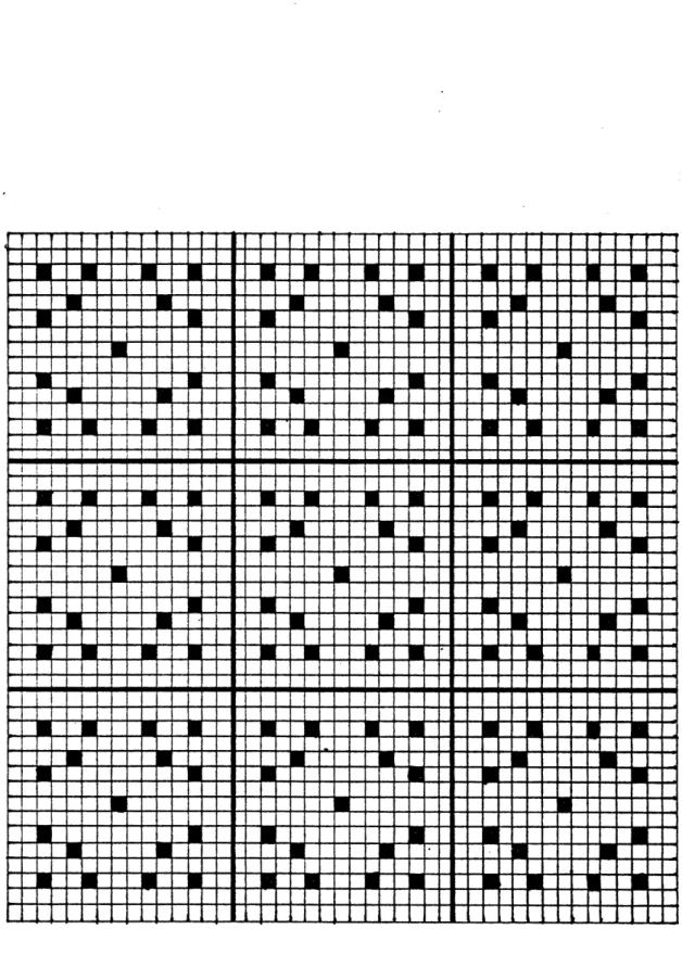
A2.1 Benchmark Problem 1

3 x 3, Symmetric Checkerboard, Unrodded A2-3

A2.2 Benchmark Problem 2

3 x 3, Symmetric Checkerboard, Rodded

Fuel 1 A2-4

A2.3 Benchmark Problem 3

3 x 3, Asymmetric Checkerboard, Rodded

Fuel 1 A2-5

A2.4 Benchmark Problem 4

3 x 3, Quarter-Core, Some Assemblies

Rodded A2-6

A2.5 Benchmark Problem 5

True Infinite Checkerboard, Unrodded A2-7 A2.6 Benchmark Problem 6

4 x 4, Quarter-Core, Unrodded, Explicit

Baffle A2-8

A2.7 Benchmark Problem 7

3. x 3, Center Node Heterogeneous, Unrodded A2-9

A2.8 Benchmark Problem 8

3 x 3, Quarter-Core, Some Assemblies Rodded, Phi = 0 Boundary Conditions on

2 Sides A2-10

A4.1 Results for kff and Normalized Power

Densities for Benchmark Problem 1 A4-3 A4.2 Results for keff and Normalized Power

Densities for Benchmark Problem 2 A4-4

A4.3 Results for k and Normalized Power effo

Figure

A4.4 Results for keff and Normalized Power Densities for Benchmark Problem 4 A4.5 Results for keff and Normalized Power

Densities for Benchmark Problem 5 A4.6 Results for keff and Normalized Power

Densities for Benchmark Problem 6

A6.0.1 Geometry for a CHIME Interpolation A6.0.2 Surface and Corner Point Labeling

of a Node n = 1,2,3 4

A7.1 CARILLON Geometry

A8.1 CAMPANA Geometry

A12.0 Plot Orientation Example: The Reference Fast Flux in Node 4 of Benchmark Problem 6 A12.1 Reference Benchmark A12.2 Reference Benchmark A12.3 Reference Benchmark A12.4 Reference Benchmark A12.5 Reference Benchmark A12.6 Reference Benchmark A12.7 Reference Benchmark

Fast Flux for Node 5 of Problem 5

Thermal Flux for Node 5 Problem 5

Fast Flux. for Node 4 of Problem 6

Thermal Flux for Node 4 Problem 6

Fast Flux for Node 6 of

Problem 6

Thermal Flux for Node 6 Problem 6

Fast Flux for Node 7 of Problem 6 of of of Page A4-6 A4-7 A4-8 A6-3 A6-5 A7-2 A8-2 A12-3 A12-6 A12-7 A12-9 Al 2-10 A12-ll A12-12 A12-13

Figure Page A12.8 Reference Thermal Flux for Node 7 of

Benchmark Problem 6 A12-14

A12.9 Reference Fast Flux for Node 8 of

Benchmark Problem 6 A12-15

Al2.10 Reference Thermal Flux for Node 8 of

Benchmark Problem 6 A12-16

A12.11 Reference Fast Flux for Node 10 of

Benchmark Problem 6 A12-17

A12.12 Reference Thermal Flux for Node 10 of

Benchmark Problem 6 A12-18

A12.13 Reference Fast Flux for Node 11 of

Benchmark Problem 6 A12-19

A12.14 Reference Thermal Flux for Node 11 of

Benchmark Problem 6 Al2-20

A12.15 Reference Fast Flux for Node 12 of

Benchmark Problem 6 A12-21

A12.16 Reference Thermal Flux for Node 12 of

Benchmark Problem 6 A12-22

A12.17 Reference Fast Flux for Node 13 of

Benchmark Problem 6 A12-23

A12.18 Reference Thermal Flux for Node 13 of

Benchmark Problem 6 A12-24

A12.19 Reference Fast Flux for Node 14 of

Benchmark Problem 6 A12-25

A12.20 Reference Thermal Flux for Node 14 of

Benchmark Problem 6 Al2-26

A12.21 Reference Fast Flux for Node 15 of

Benchmark Problem 6 A12-27

A12.22 Reference Thermal Flux for Node 15 of

Benchmark Problem 6 A12-28

A12.23 Reference Fast Flux for Node 16 of

Benchmark Problem 6 A12-29

A12.24 Reference Thermal Flux for Node 16 of

Figure Page A12.25 Reference Fast Flux for Node 5 of

Benchmark Problem 7 A12-32

A12.26 Reference Thermal Flux for Node 5 of

Benchmark Problem 7 A12-33

A12.27 Reference Fast Flux for Node 5 of

Benchmark Problem 8 A12-35

A12.28 Reference Thermal Flux for Node 5 of A12-36 Benchmark Problem 8

A13.1 Fast Assembly Flux for an Unrodded

Fuel 1 Assembly A13-3

A13.2 Thermal Assembly Flux for an Unrodded

Fuel 1 Assembly A13-4

A13.3 Fast Assembly Flux for a Rodded

Fuel 1 Assembly A13-5

A13.4 Thermal Assembly Flux for a Rodded

Fuel 1 Assembly A13-6

A13.5 Fast Assembly Flux for an Unrodded

Fuel 2 Assembly A13-7

A13.6 Thermal Assembly Flux for an Unrodded

Fuel 2 Assembly A13-8

A13.7 Fast Assembly Flux for a Rodded

Fuel 2 Assembly A13-9

A13.8 Thermal Assembly Flux for a Rodded

Fuel 2 Assembly A13-10

A14.1 Fast Extended-Assembly Flux for Node 4

of Benchmark Problem 6 A14-4 A14.2 Thermal Extended-Assembly Flux for

Node 4 of Benchmark Problem 6 A14-5 A14.3 Fast Extended-Assembly Flux for Node 7

of Benchmark Problem 6 A14-6

A14.4 Thermal Extended-Assembly Flux for

Figure Page A14.5 Fast Extended-Assembly Flux for Node 8

of Benchmark Problem 6 Al4-8

A14.6 Thermal Extended-Assembly Flux for

Node 8 of Benchmark Problem 6 A14-9 A14.7 Fast Extended-Assembly Flux for

Node 10 of Benchmark Problem 6 A14-10 A14.8 ° Thermal Extended-Assembly Flux for

Node 10 of Benchmark Problem 6 A14-11 A14.9 Fast Extended-Assembly Flux for

Node 11 of Benchmark Problem 6 A14-12 A14.10 Thermal Extended-Assembly Flux for

Node 11 of Benchmark Problem 6 A14-13

A14.11 Fast Extended-Assembly Flux for

Node 12 of Benchmark Problem 6 A14-14 A14.12 Thermal Extended-Assembly Flux for

Node 12 of Benchmark Problem 6 A14-15 A14.13 Fast Extended-Assembly Flux for

Node 15 of Benchmark Problem 6 A14-16 A14.14 Thermal Extended-Assembly Flux for

Node 15 of Benchmark Problem 6 A14-17 A14.15 Fast Extended-Assembly Flux for

Node 16 of Benchmark Problem 6 A14-18 A14.16 Thermal Extended-Assembly Flux for

Node 16 of Benchmark Problem 6 A14-19

A15.1 Reference Fast Form Function for

Node 5 of Benchmark Problem 5 A15-4 A15.2 Reference Thermal Form Function for

Node 5 of Benchmark Problem 5 A15-5 A15.3 Reference Fast Form Function for

Node 6 of Benchmark Problem 6 A15-7 A15.4 Reference Thermal Form Function for

Figure Page A15.5 Reference Fast Form Function for

Node 11 of Benchmark Problem 6 A15-9 A15.6 Reference Thermal Form Function for

Node 11 of Benchmark Problem 6 A15-10

Al5.7 Reference Fast Form Function .for

Node 13 of Benchmark Problem 6 A15-11 A15.8 Reference Thermal Form Function for

Node 13 of Benchmark Problem 6 A15-12 A15.9 Reference Fast Form Function for

Node 14 of Benchmark Problem 6 A15-13

A15.10 Reference Thermal Form Function for

Node 14 of Benchmark Problem 6 A15-14

A15.11 Reference Fast F.orm Function for

Node 5 of Benchmark Problem 7 A15-16

A15.12 Reference Thermal Form Function for

Node 5 of Benchmark Problem 7 A15-17

A15.13 Reference Fast Form Function for

Node 5 of Benchmark Problem 8 A15-19 A15.14 Reference Thermal Form Function for

Node 5 of Benchmark Problem 8 A15-20

A16.1 Reference Fast Form Function Based on an Extended Assembly Calculation

for Node 7 of Benchmark Problem 6 A16-4 A16.2 Reference Thermal Form Function Based

on an Extended Assembly Calculation

for Node 7 of Benchmark Problem 6 A16-5 A16.3 Reference Fast Form Function. Based

on an Extended Assembly Calculation

for Node 10 of Benchmark Problem 6 A16-6

A16.4 Reference Thermal Form Function Based on an Extended Assembly Calculation

Figure Page A16.5 Reference Fast Form Function Based

on an Extended Assembly Calculation

for Node 11 of Benchmark Problem 6 A16-8 A16.6 Reference Thermal Form Function Based

on an Extended Assembly Calculation

for Node 11 of Benchmark Problem 6 A16-9 A16.7 Reference Fast Form Function Based

on an Extended Assembly Calculation

for Node 15 of Benchmark Problem 6 A16-10 A16.8 Reference Thermal Form Function Based

on an Extended Assembly Calculation

for Node 15 of Benchmark Problem 6 A16-11

A17.1 Percent Error in the Fast Recon-structed Flux Based on a 9-Term, Bi-Quadratic Form Function for

Node 5 of Benchmark Problem 7 A17-3 A17.2 Percent Error in the Thermal

Recon-structed Flux Based on a 9-Term, Bi-Quadratic Form Function for

Node 5 of Benchmark Problem 7 A17-4

A18.1 Percent Error in the Fast Recon-structed Flux Based on a 25-Term, Bi-Quartic Form Function for

Node 5 of Benchmark Problem 7 A18-3 A18.2 Percent Error in the Thermal

Recon-structed Flux Based on a 25-Term, Bi-Quartic Form Function for

Node 5 of Benchmark Problem 7 A18-4 A18.3 Percent Error in the Fast

Recon-structed Flux Based on a 25-Term, Bi-Quartic Form Function for

Node 5 of Benchmark Problem 8 A18-5 A18.4 Percent Error in the Thermal

Recon-structed Flux Based on a 25-Term, Bi-Quartic Form Function for

Figure Page Al9.1 Percent Error in the Fast

Recon-structed Flux from FORTE for Node 5 of Benchmark Problem 5 (FORTE input

data from QUANDRY-ADF-AXS/CHIME) Al9-5 Al9.2 Percent Error in the Thermal

Recon-structed Flux from FORTE for Node 5 of Benchmark Problem 5 (FORTE input

data from QUANDRY-ADF-AXS/CHIME ) A19-6 A19.3 Percent Error in the Fast

Recon-structed Flux from FORTE for Node 5 of Benchmark Problem 7 (FORTE input

data from QUANDRY-ADF-AXS/CHIME) A19-8

A19.4 Percent Error in the Thermal Recon-structed Flux from FORTE for Node 5 of Benchmark Problem 7 (FORTE input

data from QUANDRY-ADF-AXS/CHIME) A19-9

A19.5 Percent Error in the Fast Recon-structed Flux from FORTE for Node 10 of Benchmark Problem 6 (FORTE input

data from QUANDRY-ADF-AXS/CAMPANA) A19-11 A19.6 Percent Error in the Thermal

Recon-structed Flux from FORTE for Node 10 of Benchmark Problem 6 (FORTE input

data from QUANDRY-ADF-AXS/CAMPANA) A19- 12 A19.7 Percent Error in the Fast

Recon-structed Flux from FORTE for Node 11 of Benchmark Problem 6 (FORTE input

data from QUANDRY-ADF-AXS/CAMPANA) A19-13 A19.8 Percent Error in the Thermal

Recon-structed Flux from FORTE for Node 11 of Benchmark Problem 6 (FORTE input

data from QUANDRY-ADF-AXS/CAMPANA) A19-14 A19.9 Percent Error in the Fast

ReCon-structed Flux from FORTE for Node 13 of Benchmark Problem 6 (FORTE input

data from QUANDRY-ADF-AXS/CAMPANA) A19-15 A19.10 Percent Error in the Thermal

Recon-structed Flux from FORTE for Node 13 of Benchmark Problem 6 (FORTE input

Figure Page A19.11 Percent Error in the Fast

Recon-structed Flux from FORTE for Node 14 of Benchmark Problem 6 (FORTE input

data from QUANDRY-ADF-AXS/CAMPANA) A19-17 A19.12 Percent Error in the Thermal

Recon-structed Flux from FORTE for Node 14

of Benchmark Problem 6 (FORTE input

data from QUANDRY-ADF-AXS/CAMPANA) A19-18 A19.13 Percent Error in the Fast

Recon-structed Flux from FORTE for Node 15 of Benchmark Problem 6 (FORTE input

data from QUANDRY-ADF-AXS/CAMPANA) A19-19 A19.14 Percent Error in the Thermal

Recon-structed Flux from FORTE for Node 15 of Benchmark Problem 6 (FORTE input

data from QUANDRY-ADF-AXS/CAMPANA) A19-20 A19.15 Percent Error in the Fast

Recon-structed Flux from FORTE for Node 11 of Benchmark Problem 6 (FORTE input data from Reference Form Functions

in Appendix 16) A19-22

Al9.16 Percent Error in the Thermal

Recon-structed Flux from FORTE for Node 11 of Benchmark Problem 6 (FORTE input data from Reference Form Functions

in Appendix 16) A19-23

A19.17 Percent Error in the Fast Recon-structed Flux from FORTE for Node 15 of Benchmark Problem 6 (FORTE input data from Reference Form Functions

in Appendix 16) A19-24

A19.18 Percent Error in the Thermal Recon-structed Flux from FORTE for Node 15 of Benchmark Problem 6 (FORTE input data from Reference Form Functions

in Appendix 16) A19-25

A19..19 Percent Error in the Fast Recon-structed Flux from FORTE for Node 11 of Benchmark Problem 6 (FORTE input data from Form Functions in

Figure Page A19.20 Percent Error in the Thermal

Recon-structed Flux from FORTE for Node 11 of Benchmark Problem 6 (FORTE input data from Form Functions in

Appendix 15) A19-28

A20.1 The Reconstructed Fast Form Function from FORTE for Node 5

of Benchmark Problem 5 (FORTE input

data from QUANDRY-ADF-AXS/CHIME) A20-4 A20.2 The Reconstructed Thermal Form

Function from FORTE for Node 5

of Benchmark Problem 5 (FORTE input

data from QUANDRY-ADF-AXS/CHIME) A20-5 A20.3 The Reconstructed Fast Form

Function from FORTE for Node 5

of Benchmark Problem 7 (FORTE input

data from QUANDRY-ADF-AXS/CHIME) A20-7 A20.4 The Reconstructed Thermal Form

Function from FORTE for Node 5

of Benchmark Problem 7 (FORTE input

data from QUANDRY-ADF-AXS/CHIME) A20-8 A20.5 The Reconstructed Fast Form

Function from FORTE for Node 10 of Benchmark Problem 6 (FORTE input

data from QUANDRY-ADF-AXS/CAMPANA) A20-10 A20.6 The Reconstructed Thermal Form

Function from FORTE for Node 10 of Benchmark Problem 6. (FORTE input

data from QUANDRY-ADF-AXS/CAMPANA) A20-11 A20.7 The Reconstructed Fast Form

Function from FORTE for Node 11 of Benchmark Problem 6 (FORTE input

data from QUANDRY-ADF-AXS/CAMPANA) A20-12 A20.8 The Reconstructed Thermal Form

Function from FORTE for Node 11 of Benchmark Problem 6 (FORTE input

data from QUANDRY-ADF-AXS/CAMPANA) A20-13 A20.9 The Reconstructed Fast Form

Function from FORTE for Node 13 of Benchmark Problem 6 (FORTE input

Figure Page A20.10 The Reconstructed Thermal Form

Function from FORTE for Node 13 of Benchmark Problem 6 (FORTE input

data from QUANDRY-ADF-AXS/CAMPANA) A20-15 A20.11 The Reconstructed Fast Form

Function from FORTE for Node 14 of Benchmark Problem 6 (FORTE input

data from QUANDRY-ADF-AXS/CAMPANA) A20-16 A20.12 The Reconstructed Thermal Form

Function from FORTE for Node 14 of Benchmark Problem 6 (FORTE input

data from QUANDRY-ADF-AXS/CAMPANA) A20-17 A20.13 The Reconstructed Fast Form

Function from FORTE for Node 15 of' Benchmark Problem 6 (FORTE input

data from QUANDRY-ADF-AXS/CAMPANA) A20-18 A20.14 The Reconstructed Thermal Form

Function from FORTE for Node 15 of Benchmark Problem 6 (FORTE input

data from QUANDRY-ADF-AXS/CAMPANA) A20-19 A20.15 The Reconstructed Fast Form

Function from FORTE for Node 11 of Benchmark Problem 6 (FORTE input data from Reference Form

Functions in Appendix 16) A20-21

A20.16 The Reconstructed Thermal Form Function from FORTE for Node 11 of Benchmark Problem 6 (FORTE input data from Reference Form

Functions in Appendix 16) A20-22

A20.17 The Reconstructed Fast Form

Function from FORTE for Node 15 of Benchmark Problem 6 (FORTE input data from Reference Form

Functions in Appendix 16) A20-23

A20.18 The Reconstructed Thermal Form Function from FORTE for Node 15 of Benchmark Problem 6 (FORTE input data from Reference Form

Figure Page A20.19 The Reconstructed Fast Form

Function from FORTE for Node 11 of Benchmark Problem 6 (FORTE input data from Reference Form Functions in

Appendix 15) A20-26

A20.20 The Reconstructed Thermal Form Function from FORTE for Node 11

of Benchmark Problem 6 (FORTE input data from Reference Form Functions in

LIST OF TABLES

Table Page

4.1 CHIME Corner Point Flux Interpolation

Results for Benchmark Problem 5 4-13 4.2 CHIME Corner Point Flux Interpolation

Results for Benchmark Problem 7 4-14 4.3 . CHIME Corner Point Flux Interpolation

Results for Benchmark Problem 8 .4-16 4.4 CARILLON Corner Point Flux

Interpolation Results for

Benchmark Problem 5 4-20

4.5 CARILLON Corner Point Flux Interpolation Results for

Benchmark Problem 7 4-21

4.6 CARILLON Corner Point Flux Interpolation Results for

Benchmark Problem 8 4-22

4.7 CARILLON Corner Point Flux Interpolation Results for

Benchmark Problem 6 4-24

4.8 CAMPANA Corner Point Flux Interpolation Results for

Benchmark Problem 6 4-29

5.1 Bi-Quadratic Method Flux Reconstruction Results for

Benchmark Problem 7 5-4

5.2 Bi-Quartic Method Flux Reconstruction

Resutls for Benchmark Problems 5,7 and 8 5-9

6.1 The Maximum Percent Error in the FORTE Heterogeneous Flux Reconstructions for

Table Page Al.1 Pin-Cell Homogenized Cross

Section Sets Al-3

A3.1 ADF/AXS for Unrodded PWR Fuel

Assemblies A3-4

A3.2 ADF/AXS for Rodded (CR1) PWR

Fuel Assemblies A3-6

A3.3 ADF/AXS for Rodded (CR2) PWR

Fuel Assemblies A3-8

A3.4 ADF/AXS Using an Extended Assembly Calculation for an Unrodded Fuel 1 Assembly and a

Baffle/Water Node A3-10

A3.5.1 ADF/AXS Using an Extended

Assembly Calculation for Nodes

Near a Jagged Baffle, Nodes 1 and 2 A3-12 A3.5.2 ADF/AXS Using an Extended

Assembly Calculation for Nodes

Near a Jagged Baffle, Nodes 3 and 4 A3-13 A3.5.3 ADF/AXS Using an Extended

Assembly Calculation for Nodes

Near a Jagged Baffle, Nodes 5 and 6 A3-14

A5.1.1 Estimate of Spatial Truncation Error for an Unrodded Fuel-l Assembly

Calculation A5-4

A5.1.2 A Comparison of the Reference QUANDRY/CHIME Corner Point Fluxes vs. the Reference PDQ-7 Corner

Point Fluxes for Benchmark Problem 5 A5-6 A5.2.1 Estimate of Spatial Truncation

Error for Benchmark Problem 6 A5-8 A5.3.1 A Comparison of the Reference

QUANDRY/CHIME Corner Point Fluxes vs. the Reference PDQ-7 Corner

Table Page A5.4.1 A Comparison of Reference Corner

Points for Node 5 of Benchmark

Problem 8 A5-12

A6.O.1 Thirty-Two Conditions on the Products

Chapter 1

INTRODUCTION

"1.1 OVERVIEW

There are strong economic and safety incentives

in the utility industry to perform accurate and reasonably inexpensive multidimensional reactor calculations. By accurately calculating the multidimensional behavior of reactors, the utilities can gain safety benefits from an increased confidence in plant safety margins. Direct economic gains may accrue from improved fuel management and the possible relaxation of some plant margins due to increased confidence in the knowledge of plant operating conditions.

Finite-difference solutions of the group diffusion equations [1, pgs. 156-168] are commonly employed in the nuclear industry for the calculation of spatial power distributions within reactors. Such finite-difference methods have been automated within many computer codes. The utility industry standard is prbbably the PDQ-7 code

[2] which was originally developed at Bettis Atomic Power Laboratory for use in the US Navy reactor program.

Unfortunately, for realistic three-dimensional thermal-reactor problems, with accuracy requirements for average

assembly powers of one percent, these methods require a huge number of spatial mesh points. This leads to

excessive computing times which preclude the use of routine, three-dimensional PDQ-7 calculations in the utility industry. Planar, two-dimensional PDQ-7

calculations are routinely performed. However, even here the computing cost quickly runs into the thousands of dollars. Thus more efficient and faster methods would surely be welcomed.

It is conceivable that -as computers become more

efficient and with further advances in parallel processors that routine three-dimensional PDQ-7 calculations will become a reality and two-dimensional PDQ-7 calculations may be made considerably less expensive [3]. In the

interim, a number of other approaches are being used to derive the multidimensional behavior of operating reactors. These approaches include synthesis methods [4], finite

element techniques [5], response matrix methods [6],

nodal methods [7] and combinations of these techniques [8]. It is the use of nodal methods to supplement fine-mesh finite-difference calculations in the analysis of PWRs which is the topic of this thesis.

1.2 HISTORICAL REVIEW OF NODAL METHOD DEVELOPMENTS The term, nodal method, is a broad one. However, most nodal methods have the following salient features. ,In the nodal approach the reactor core is partitioned

into large ( ~ 20 cm x 20 cm x 20 cm) homogeneous nodes. The essential characteristic of nodal methods is to regard as unknowns, node-integrated quantities such as volume-averaged fluxes and surface-volume-averaged currents. When the multigroup neutron diffusion equation is integrated over a typical node, a rigorous mathematical statement of neutron conservation is derived. Unfortunately, this one mathematical equation contains more than one unknown. It contains the volume-averaged flux and surface-averaged currents. Thus, auxiliary spatial-coupling equations are generally developed to solve for all the unknowns. There appears to be a myraid of ways to write the spatial-coupling equations and then solve the resulting set of coupled equations. This accounts for the large number of nodal methods in the literature. Some of these methods will now be reviewed.

One of the oldest nodal methods is FLARE [9]. The FLARE method is usually implemented in one energy group.

Spatial coupling is expressed in terms of leakage probabilities which are found from a crudely derived

transport kernel. Even though the FLARE methodology lacks a rigorous theoretical foundation, there is much experience in the utility industry in using

FLARE-based codes such as EPRI-Node B and EPRI-Node P

[10].

An improved class of nodal techniques are the one-and-a-half group methods. These methods were first developed in the late 1960's and early 1970's. They are incorporated in the computer codes, TRILUX, PRESTO and CETRA [111. In these codes, various artful methods, some of which involve auxiliary fine-mesh

calculations, have been devised to determine

coupling parameters. These coupling parameters relate surface currents to nodal fluxes and thus have the effect of eliminating the surface currents, leaving only a system of equations involving nodal fluxes to be solved iteratively. These methods are of limited accuracy because only the nodal fluxes are involved in the global solution, when in fact both the nodal

fluxes and surface currents (or coupling parameters) should be updated as the iterative global solution

proceeds. One-and-a-half group methods are also widely used by utilities.

During the last ten years, a third class of nodal methods have been developed which Professor Dorning [7] labels as "modern nodal methods". These methods differ from their predecessors in that they are based upon systematic, rigorous mathematical foundations. These include the nodal collision probability method, nodal synthesis method, partial current balance method, flux expansion method, nodal expansion method, polynomial method, nodal Green's function method and the analytic nodal method.

In this thesis, the analytic nodal method is

utilized. It originated at M.I.T. in the work of Shober and Henry [12], although variations of the M.I.T. work have recently appeared in t'he literature [13]. In the analytic nodal method, a one-dimensional diffusion equation is derived for each of the three coordinate directions by integrating the multigroup diffusion equation over the two directions transverse to the direction of interest. The required flux-current,

spatial-coupling relationships are found by solving these one-dimensional diffusion equations. Unfortunately, to do this an assumption must be made concerning the trans-verse leakages from the nodes. It is the treatment of the transverse leakages that is the one clearly identified approximation inherent in the analytic nodal method. As originally implemented by Shober and Henry the analytic nodal method was limited to two dimensions and used a flat transverse leakage approximation. Greenman, Smith and Henry [14, 15, 161 extended the analytic nodal method to three dimensions. They also incorporated a quadratic transverse leakage approximation as suggested by Finneman

[17]. The resulting computer code was called QUANDRY [16]. Thus, with the advent of modern nodal codes like

QUANDRY, the tools were at hand to solve nodal reactor problems quickly and efficiently. Such nodal problems are ones in which the reactor is represented as large

homogenized nodes, either by design, or through the use of equivalent diffusion theory parameters [1, pgs. 427-457). To avoid the whole question of spatial homogenization and the generation of equivalent diffusion theory parameters

These included the two- and three-dimensional IAEA

problems [18], the two-dimensional LRA problem [19], and the three-dimensional LMW problem [20]. The modern

nodal methods were applied to these problems [7, 16] with impressive results. The nodal methods proved to be at least two orders of magnitude more computationally ef-ficient than standard finite-difference techniques.

Furthermore, this gain in computational speed was accom-plished without sacrificing accuracy. Nodal powers for these benchmarks were found to within a few percent.

1.3 A REVIEW OF SPATIAL HOMOGENIZATION OF PWR ASSEMBLIES

In this thesis the analytic nodal method in QUANDRY is applied to the neutronic analysis of pressurized water reactors (PWRs). To do this for realistic cases, a method of spatial homogenization had to be applied to the

fuel assemblies making up the PWRs. In this section, the spatial homogenization problem is discussed.

The first part of the spatial homogenization problem is called pin-cell homogenization. A typical PWR assembly is square and contains 15x15, 16x16 or 17x17 pins.

Each fuel pin is made of Zircaloy tubes which have an outer diameter of about 1 cm. The tubes are typically about 4 m long and they are filled with about 3.8 m of

sintered uranium dioxide pellets. A pin-cell is made up of the uranium pellets, the Zircaloy rod and the coolant-moderator associated with the fuel rod. In general, the pin-cell homogenization consists of finding equivalent diffusion theory parameters for each pin-cell. This is usually done through the use of collision theory methods

[21]. Pin-cell homogenization is a science in itself and it is not the intent of this thesis to examine pin-cell homogenization methods. Thus, this analysis starts with a reasonable set of pin-cell homogenized cross sections

for two fuel types, water, control rod and a steel baffle. See Appendix 1.

By assigning one of the reference, pin-cell-homogen-ized cross section sets in Appendix 1 to each homogenpin-cell-homogen-ized pin-cell in a typical PWR assembly, a heterogeneous

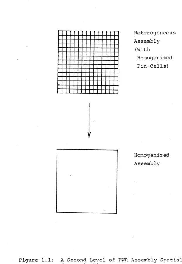
Figure 1.1: A Second Level of PWR Assembly Spatial Homogenization Heterogeneous Assembly (With Homogenized Pin-Cells) Homogenized Assembly

To utilize a nodal code like QUANDRY, a second level of homogenization must be performed. The heterogeneous assembly configuration must be spatially homogenized. For PWRs this can be done by performing two-dimensional assembly criticality calculations based on zero-net-current boundary conditions. The assembly geometry for these calculations is heterogeneous as shown at the top of Figure 1.1. Each fuel-element-cell, control-rod-cell, water hole, etc., within the assembly is represented as a homogenized pin-cell. The result of this procedure is a single set of homogenized parameters which represent the entire PWR assembly. The assembly calculation also yields the heterogeneous assembly flux, Ag(x,y), g = 1,2. Once this has been done for each unique assembly type in a PWR, then a nodal code may easily be employed.

The reactor physics community realized the importance of finding a systematic method to accomplish this second level of spatial homogenization and much work was

performed throughout the 1970's on this topic [22, 23, 24, 25]. In this thesis, the spatial homogenization method used is that of Koebke [26] as extended by Smith

[27]. This spatial homogenization method is called

assembly calculations described in the previous paragraph can be advantageously employed to perform the spatial homogenization. This is described in Chapter 2.

Smith incorporated nodal equivalence theory (NET) into the computer code QUANDRY and then applied it to

several boiling water reactor (BWR) benchmark problems [28]. Cheng and Henry [29] incorporated response matrix techniques into nodal equivalence theory as a practical approach to iterative BWR assembly homogenization.

Also, Henry and the author [29] applied NET to some rodded PWR benchmark problems. In this thesis, NET is applied to several rodded and unrodded PWR benchmark problems and results are presented. See Chapter 3.

Thus, when Smith completed his work, the nodal

code QUANDRY looked fairly complete. It was computation-ally efficient and a consistent spatial homogenization

scheme had been incorporated into QUANDRY. The next step was to apply QUANDRY fto depletion problems. Unfortunately, to perform a detailed depletion of a PWR core, one must have pointwise, heterogeneous fluxes for each assembly in the core. QUANDRY supplies only volume- and surface-averaged fluxes. Clearly, if QUANDRY was to be enabled to perform a detailed core depletion and be able to pick out the hottest pin in a PWR

QUANDRY to reconstruct the pointwise heterogeneous fluxes in a core. Devising and implementing a heterogeneous flux reconstruction scheme for PWR analysis is a major part of this thesis. The next section gives an overview of this problem.

1.4 RECONSTRUCTION OF HETEROGENEOUS PWR FLUXES FROM NODAL CALCULATIONS

Figure 1.2 illustrates a global heterogeneous PWR problem. The problem is heterogeneous because a cross section set from Appendix 1 is specified for each pin-cell in each assembly making up the reactor. Thus, spatial heterogeneities such as water holes are explicitly represented in this problem.

A planar PDQ-7 calculation is commonly employed in the utility industry [30] to find the two-group, hetero-geneous fluxes for problems of this type. In this thesis, such fine-mesh PDQ-7 calculations will serve as reference calculations of the two-group, heterogeneous fluxes,

4

4

-

I

uIfI-

f

F I

heterogeneous PDQ-7 assembly calculations for each unique assembly type in the core with the results from the global homogeneous problem calculated by QUANDRY. See Figure 1.3.

The reconstruction of detailed fluxes and pin powers from nodal calculations is not a new idea [31, 32]. How-ever, the approach that has been pursued at M.I.T. [33] is different in that the Koebke/Smith equivalence theory ideas allow heterogeneous flux and current information from the homogenized global problem to be input into the flux reconstruction techniques.

Koebke and Wagner present two basic approaches to flux reconstruction [31]. These approaches are the imbedded heterogeneous assembly calculation method and the modula-tion method. The most accurate and expensive method of these two is the imbedded heterogeneous assembly calcula-tion. Such imbedded calculations can be performed in two ways. The first way is to use information from the nodal

calculation and heterogeneous assembly calculation to infer logarithmic boundary conditions at the assembly faces.

An assembly eigenvalue problem using this logarithmic boundary condition then yields the reconstructed flux. The second way is to use information from the nodal calculation and heterogeneous assembly calculation to

Figure 1.3: A Heterogeneous Assembly Problem and a Global Homogeneous Problem L 1 1

surface. An inhomogeneous boundary source problem

then yields the reconstructed flux. Clearly, the accuracy of-the imbedded heterogeneous assembly approach depends entirely on how accurately the logarithmic boundary condition or inhomogeneous boundary source is inferred.

Koebke and Wagner [31] and Jonsson, Grill and Rec [32] report excellent flux reconstruction results by using partial in-currents from the nodal calculations to derive boundary sources for an inhomogeneous boundary

source problem. This appears to be due to their success at accurately approximating the reference partial in-current distributions from information from the nodal calculations and heterogeneous assembly calculations. Partial out-current distributions are not well fit and thus the logarithmic boundary condition approach, which requires both partial in- and out-currents,did not fare as well [31].

At M.I.T. Parsons [34] has successfully calculated the inhomogeneous boundary source by assuming that

fluxes on the surfaces of PWR assemblies are quadratic. Parsons' quadratic surface fluxes are inferred using only information from the nodal calculation. Finck [35] has calculated the inhomogeneous boundary source by

assuming that the ratio, 9(x,y)/A (x,y), on the surfaces of BWR bundles is quadratic. Thus, Finck uses information from both the nodal calculation and the heterogeneous

assembly calculation.

Imbedded heterogeneous assembly calculations appear to yield reconstructed heterogeneous pin power distri-butions to within a few percent. However, they are relatively expensive since they require auxiliary, fine-mesh assembly calculations.

The second approach to flux reconstruction is called the modulation method by Koebke and Wagner [31]. For each assembly they find a pin power distribution from a heterogeneous assembly calculation. Information from the global nodal calculation is used in a local interpolation to find a smooth power distribution. The product of the pin power distribution and the smooth power distribution yields the shape of the modulated heterogeneous power

distribution. A renormalization is applied so the assembly average of the final modulated heterogeneous power distri-bution matches the assembly average .power from the nodal calculation.

In this thesis, the approach taken to heterogeneous PWR flux reconstruction is called the form function method.

It is closer to the modulation method than it is to the imbedded heterogeneous assembly calculation method. Its essence is to search for a form function, F (x,y), that multiplicatively corrects the assembly flux, A g(x,y), such that the product A (x,y) F (x,y) reconstructs

g g

the global heterogeneous flux, 9 (x,y), within the assembly. The equation,

4g(x,y)

defines the reference form function, F (x,y). However, g

this equation is useless in helping to find approximations to F (x,y) since g (x,y) is not known (without having

done the expensive reference global calculation). Since the effects of local heterogeneities on flux shapes are represented in both the global heterogeneous flux, 9(x,y), and the assembly flux, A (x,y), the form function, F (x,y),

g g

is spatially smooth. Thus, the form function method consists of finding analytic functions to approximate the reference F (x,y) in equation 1.1. The reconstructed

g

analytic form function is called FR(x,y). Once FR(x,y)

g g

is found, the reconstructed heterogeneous flux, R

g (x,y), is g

R _{(x,y) =} A (x,v) _{FR (x,y) (1.2)}

In general, the analytic form function, FR(x,y) g

contains coefficients whose magnitudes are determined by forcing the reconstructed flux in equation 1.2 to .match heterogeneous global flux information derived from

the global homogeneous QUANDRY problem. Specifically, for each assembly,QUANDRY yields good approximations of the heterogeneous volume-averaged group-flux and the heterogeneous surface-averaged group-currents and group-fluxes.

It was found that using only these integral quantities was not enough information to determine all the coeffi-cients of some analytic form functions. Thus in Chapter 4 of this thesis, methods of interpolating the heterogeneous corner point fluxes at each of the four corners of a PWR assembly are presented. These interpolation methods are tested on several benchmark problems and results are presented.

In Chapter 5, the analytic form function, F R(x,y), is

g

expressed in terms of various polynomial functions. Point-wise flux reconstructions are performed and results are presented for several PWR benchmark problems.

In Chapter 6, the group diffusion equations are used to derive a coupled set of differential equations for the reference form functions, F (x,y), g = 1,2. A solution technique is employed to solve the coupled set of equations in an approximate fashion. The resulting solution yields a non-polynomial, analytic form function, F (x,y),

g

g = 1,2. Pointwise flux reconstructions are performed and results are presented for several PWR benchmark problems.

Chapter 7 contains conclusions and recommendations for future work.

1.5 SUMMARY AND OBJECTIVE

This chapter has reviewed nodal method developments. Modern nodal methods were first developed in the 1970's. To benchmark these methods, nodal problems were devised

in which the homogenized diffusion theory parameters were assumed known. The nodal code employed in this thesis is QUANDRY. The next step was to develop methods for finding homogenized diffusion theory parameters. The nodal

equivalence ideas of Koebke as extended and implemented into QUANDRY by Smith are used. The reconstruction of the heterogeneous flux was the next problem that needed to be solved to make QUANDRY more useful for PWR analysis.

It is the objective of this thesis to apply the analytic nodal method and nodal equivalence theory as embodied in QUANDRY to the neutronic analysis of PWRs. This includes applying QUANDRY to the calculation of normalized assembly power distributions for PWRs and devising, implementing and testing a heterogeneous PWR

Chapter 2

A REVIEW OF THE ANALYTIC NODAL METHOD AND NODAL EQUIVALENCE THEORY

2.1 INTRODUCTION

The purpose of this chapter is to review the analytic nodal method and nodal equivalence theory as implemented in QUANDRY. The theory described in this chapter is not new. However, the concepts in this

chapter form the foundation for understanding the theory and results that make up the rest of this thesis. A more complete treatment of the analytic nodal method is

in Smith's N. E. Thesis [16]. Nodal equivalence theory is described in Smith's Ph.D. Thesis [27].

The QUANDRY nodal balance equation is presented and the QUANDRY spatial coupling equations are discussed in section 2 of this chapter. Section 3 describes nodal equivalence theory and a cross section homogenization

method through which reference diffusion theory parameters may be found. Section 4 presents inexpensive methods for

finding close approximations of the reference parameters based on fine-mesh assembly calculations. Section 5

The generalized notation employed by Smith [16,27] is used in this chapter. The global reactor problem is

treated in three-dimensional Cartesian geometry, where x, y and z represent the three coordinate directions and u, v and w serve as generalized coordinate subscripts. The spatial domain of all problems is divided into an

array of right rectangular parallelopipeds (nodes) with grid indices defined by u., vm, wn where

i = 1, 2, ... , I; u, v, w = x £, m, n = j = l, 2, ... , J; u, v, w = y k = 1, 2, ... , K; u, v, w = z.

The node (i,j,k) is defined by X E [xi , Xi+l

y E [yj Yj+l I z E [zk , Zk+l '.

The node widths are expressed as

u

h = u+ 1 - u ; u = x, y, z.

The volume of node (i,j,k) is V. . = hx hy hz

2.2 THE QUANDRY EQUATIONS 2.2.1 Introduction

The QUANDRY computer code may be used to solve a global homogeneous reactor problem as represented in Figure-1.3 of Chapter 1. The spatial domain of such homogeneous problems is divided into an array of

rectangular nodes which have homogeneous compositions. Associated with each homogenized node is a single set of node-homogenized diffusion theory parameters which

are spatially constant within each node. In this section it is assumed that these parameters are known. The

problem of finding these parameters for the general case when the reactor problem is heterogeneous is deferred until later sections of this chapter. The superscript

"hom" is used in this section as a mnemonic device to indicate that a given quantity is related to the homogeneous reactor problem.

This section presents four equations that are fundamental to the theory upon which QUANDRY is based. The first is the QUANDRY nodal balance equation for a

homogeneous node (i,j,k). The second is the differential equation for the QUANDRY one-dimensional homogeneous

fluxes. The third and fourth are equations for the

2.2.2 The Nodal Balance Equation

The three-dimensional, multigroup neutron diffusion equation for the global homogeneous problem is

a u, hom u gi, au i,j,k

a

hom

]

1 m(x,y,z)

•g,

1,

= total number of neutron energy groups = _{diffusion coefficient for group g, -i}

direction u and in node (i,j,k), (cm ) han

ham (x,y,z)=

g scalar neutrbn flux in group g (cm

- 2 _{sec-i )} hom agi,j,k hom sgi,j ,k hom gi,j,k 1 hom hom fgi,j,k

Ehom = macroscopic absorption cross section for agi,j,k _{group g in node (i,j,k), (cm}- 1₎

U=X-y,

u=xfylz

hom sgi,j,k hom Xgi,j,k

Xhom

= macroscopic scattering cross section for group g in node (i,j,k), (cm- 1)

= fission spectrum for group g in node (i,j,k)

= reactor eigenvalue for the global

homogeneous problem (keff)

= the mean number of neutrons released per

fission times the macroscopic fission

cross section for group g in node (i,j,k),

-i

(cm- )

= macroscopic transfer cross section

from group g' to group g (cm-1).

The integration of equation 2.1 over the volume of the homogeneous node

hy z Lx,hom

j

X

ha,,k g'hcm

In equation 2.2, the volume-averaged flux in group g

for the homogeneous node (i,j,k) is

xi+l 1 Idx

f

dx

f

dy

The nodal face-averaged, u-directed, net leakage is

u, hom g£+l,m,n u u,hom g,m, n (2.4)

where the nodal f-ace-averaged, u-directed net current for the homogeneous node (i,j,k) is

Du , hom ,-Djk 4i,j,k u, hom gi,j,k m+1 n+1 d .~homr(uvw) dv dw QýOm _{(u kvw)} w m n h 'hW m n u = x, y, z v u

w u

3

v.

gi,j,k

5

f

Equation 2.2 is a rigorous statement of neutron conservation within node (i,j,k). However, the utility of equation 2.2 is limited unless additional relationships can be specified which involve both the nodal face-averaged

uhom

net leakages, L , and the nodal volume-averaged gi,j,k

hom

fluxes , . The required relationships ij,k

are called spatial coupling equations.

The first step in deriving the QUANDRY spatial

coupling equations is to formulate a differential equation which can be solved for the one-dimensional, homogeneous QUANDRY fluxes. That differential equation is presented in the next subsection of'this chapter.

2.2.3 Differential Equation for the One-Dimensional Homogeneous Fluxes The differential equation for the one-dimensional

homogeneous fluxes in QUANDRY is determined by integrating the diffusion equation over the two directions transverse to the direction of interest. This yields for the direction u (= x, y, z) and node (Z,m,n) - hv hw Du, hom m n _{g ,mn} hv hw E homrn m n Rg 1, m, n 2 _{u,hom (u)} S(u) u2 g,m,n u, hom 9g,m,n G v w G hom m n gg' g'9g g , m, n Vm+1

DVhom

i dv

ham

Iu,ham(u) +

fg',

Z(u)

]

+

DW,hom

dv

_dw

v

u

(u,v,w)

Vm+ 1

uhom

_{(u) =}

_h

_dv

T

dw

g

(u,v,W)

g

,m,n

is the one-dimensional homogenized QUANDRY flux in group g and in direction u for node (£,m,n).

Equation 2.5 may be written in a more compact form by. defining the directionally dependent transverse leakages

Lv,hom(u) L (u) = g£,m,n V_m+1 - Dv'hom _gk,m,n dv m n+l

idw

dw

(u,v,w)

vw

v

u

Note that when the transverse leakage in equation 2.7 is integrated over [u₂ , u +11 and divided by hu it yields where

hu

_k

u

which is the nodal face-averaged, v-directed, net leakage. The sum of two net leakages transverse to the direction u, per unit u, divided by hV

m u,hom 1(u) S (u) = ,km,rn h m v, hom I_ L ,hom (u) + 1 g£,m,n hw n w, hom L m (u) gRm,n u = x, y, z v u

w u 3 v.

By using the definitions in equations 2.7 and 2.9, the differential equation 2.5 becomes

SDu, hom °gz,m,n 2 a ₂ u, hom rn ,m (u) au2 g ,m,n

hom u,hom (u) Rg£,m,n g9 _,m,n RHS m (u) gz,m,n

G

Thus, the right-hand side of the differential equation 2.1o is composed of the difference of the out-of-group source term and the total transverse leakage term.

An analytic solution for the one-dimensional

homogeneous group-flux, ₄u,hom (u), would be possible g,m,n

if the right-hand side of equation 2.10 were known. Such a solution could then be utilized to provide the required spatial coupling relationships between homogenized net leakages and node-averaged fluxes. Unfortunately, RHSuhom (u) in equation 2.10 is not known. Thus an

g,m, n

approximation is required.

At this point, the nodal analysis can take many branches. For example, Smith [36] indicates that if

uhom

RHSuh (u) could be represented as spatially flat, then g,m,n

a multigroup approach to the solution of equation 2.10

could be taken in which each group is treated sequentially. Such an approach would be invaluable if the total number of groups, G, is much greater than two. However, the purpose of this thesis is tQ perform neutronic analysis of PWRs. For that purpose, G = 2 is satisfactory for

many calculations. Thus, in QUANDRY, a two-group approach is taken in which the group-fluxes are solved for

simultaneously, not sequentially. This is accomplished by moving the out-of-group source term on the right-hand side of equation 2.10 to the left-hand side, leaving only the total transverse leakage term on the right.

The resulting differential equation for the one-dimensional homogenized QUANDRY fluxes is written in matrix form as u, hom -[ D,m, n R, m, n 2 _I u,hom (u) 2 Z ,m,n

au

Z ,m, n = - [ S u,hom (u)Z,m,n

m

u

=

x,

y,

W 4

V

u

is a column vector of length G

containing homogenized one-dimensional fluxes

is a diagonal G x G matrix containing directionally dependent, homogenized diffusion coefficients

is a column vector of length G contain-ing homogenized total net leakages

transverse to the direction u

hom [ £,m,n] hom

a[

The meanings of the terms making up the [Ehom

,,m,n

matrix are

[hom ] is a diagonal G x G matrix containing at,m,n _{macroscopic absorption cross sections}

[hom is a diagonal G x G matrix containing s£,m,n macroscopic scattering cross sections

hom

[ hom

1

g99 ,m,n macroscopic scattering cross sections for scattering from group g' to group g

Ahom is the eigenvalue of the homogeneous global reactor problem

hom

Shom is a column vector of length G

containing the fission neutron spectrum

[,hom

z,m, n

] is a column vector of length G contain-ing nu, the mean number of neutrons emitted per fission, times the

macro-scopic fission cross section.

Unfortunately, the net transverse leakage term,

[Su hom (u) ], is still not known. Thus, an approximation £,m,n

concerning it must be made so that the differential equations 2.11 can be solved for the one-dimensional