Airline crew scheduling : a group theoretic approach

AIRLINE CREW SCHEDULING:

A GROUP THEORETIC APPROACH

Herve Thiriez

Flight Transportation Laboratory, MIT Herve Thiriez

Memo FTL-M69-3 December, 1969

SET COVERING PROBLEMS SOLVED BY GROUP THEORY COMPUTATIONAL EXPERIENCE

To understand the terminology please refer to FTL-R69-l "The Airline Crew Scheduling Problem - A Group Theoretic Approach". All the problems were provided by airlines and

solved without any change in the problem definition. The computer used was the MIT IBM 360/65 with 512K core.

a) GTMP

The group theoretic method program is written in FORTRAN and linked to MPS, the IBM Mathematical Programming System. It solves all problems for which the optimal LP basis has a prime determinant or where the group is cyclic

(see R-69-1 , section 3-4). LP Time 15.6 sec. 31.8 sec. 28.2 sec. Time After LP 9.6 sec. 22.8 sec. 40.8 sec. Total Time 25.2 sec. 54.6 sec. 69 sec. S ize 104x132 104x236 67x536 AA-I AA-II AF Type Ax1l Ax=l Ax=1

b) Visual Inspection

The same problems were solved by visual inspection: -l

the LP was solved and the B a. columns were all printed J

together with the LP optimum. The optimal solution was found by visual scanning.

Size Type LP

Time

Total Time

AA-I 104x132 Axx>l 15.6 sec. 20.4 sec.

AA-II 104x236 Ax=l 31.8 sec. 39.8 sec.

AF 67x536 Ax=l 28.2 sec. 50 sec.

ASPl* AS P2* ASP3*, 32x36 27x31 69x269

)

*these problems are aircraft scheduling problems

c) Semi-BLIP Approach

For large problems and/or problems with a non-prime but small determinant (non-cyclic group), the BLIP approach

(see R69-1, section 4.2.2) is to be used. As of now, it has not been programmed; the author however used the technique by printing intermediate results and scanning visually before re-submitting the program, until the optimal solution was found and proved optimal.

If the technique were programmed, more computer time would be needed for the program to read files and do the scanning itself. However, time would be saved since the LP optimum would not have to be restored each time the program is resubmitted. According to the author's experience, the

computer times would be equivalent if everything were programmed.

Time

Type Size LP Time After LP

UAL Ax=1 117x4845 20 min. 105 sec.

Xl Ax),l 527x2800 191* min. 7.28 min.

X2 Axgl 497x2909 75* min. 14.62 min.

X3 Ax)l 1138x3533 35** min. 16.99 min.

* on a 600K 360/65 computer

** on a 812K 360/65, equivalent to at least 120 min. on a 512K

d) Semi-ABT

The automatic branching technique was designed (see R69-1, section 4.2.4) for the solution of problems with a unit cost and a non-cyclic group. A program was written which

branches automatically and re-submits the LP as often as necessary. When this branching is finished, the semi-BLIP approach was

used to solve the problem optimally.

Time Total

Size Type LP Time After LP Time

BEA-I 84x854 Ax>l 1.57 min. 2.06 min. 4.63 min.

e) Conclusions

Paragraph (c) proves that, as the author expected, the time needed to solve problems as a function of their size

increases definitely much slower than the time needed to get the LP optimum. The solution time after LP is in fact so small that it would most likely take more time for the large problems to make a cut and resolve the problem; consequently,

the author expects branch and bound and cutting plane methods to execute slower than BLIP or ABT. For GTMP, time is lost

-l

by sending all B a. columns on file and reading all of them into J

the FORTRAN program - this is caused by the lack of feasibility -l of MPS which does not allow sending out only some of the B a. columns as a function of the LP results without exchanging control from MPS to a FORTRAN program and then back; this change of control also needs some time overhead and is not interesting for small problems. However, it seems that even GTMP, the least efficient of the three techniques, is highly competitive with other existing solution techniques.

MASSACHUSETTS INSTITUTE OF TECHNOLOGY FLIGHT TRANSPORTATION LABORATORY

FTL Report R-69-1 October 1969

AIRLINE CREW SCHEDULING: A GROUP THEORETIC APPROACH

Herve Thiriez

This research was completed as a Ph.D. Thesis in the Flight Transportation Laboratory.

CORRECTIONS

Page 71 at the top, read:

z 9.

..

91 Gr

Page 67, after (2c), please add:

"...so that all the elements in (2c) are integer values ranging from 0 to (D-1). Let us index from 1 to n the non-basic columns and from (n+l) to (n+m) the basic

AIRLINE CREW SCHEDULING: A GROUP THEORETIC APPROACH

by

Herve Thiriez

Submitted to the Department of Civil Engineering on October 10, 1969 in partial fulfillment of the requirements for the degree of Doctor of Philosophy.

ABSTRACT

The problem of airline crew scheduling is studied, the different problems composing it are formulated and solution

techniques are offered.

Special emphasis is given to the set covering problem appearing in the rotation selection phase. An approach is presented, based on the group theoretic method, which allows

the fast solution of problems with large sizes.

Thesis Supervisor: Robert W. Simpson Title: Associate Professor of

Aeronautics and Astronautics

-2-ACKNOWLEDGEMENTS

My deepest appreciation goes to Professor Robert W.

Simpson for his constant supervision and helpful suggestions. To Professor Alan M. Hershdorfer who encouraged me to

pursue the Doctoral Program and assisted me through most of it, I want to express my gratitude; also, to Professor Jeremy F. Shapiro who introduced me to group theory and made this thesis possible.

Finally, my thanks go to Mrs. Betsy Gaudreau who

typed, erased, and re-typed this thesis with almost constant good humor.

TABLE OF CONTENTS Chapter No.

Introduction

I The Crew Scheduling Process 1.1 Definitions

1.2 The Crew Scheduling Process 1.3 Segment Generation

1.4 Rotation Generation

1.5 Rotation Matrix Reduction 1.6 Rotation Selection

1.7 Monthly Bids

1.8 Reserve Crew Assignment

1.9 Other Types of Crew Scheduling II Rotation Selection

2.1 Formulations

2.1.1 General Set Covering Formulation 2.1.2 Knapsack Formulation for Ax = 1 2.1.3 Network Flow Formulation

2.2 Solution Methods

2.2.1 Heuristic Methods 2.2.2 Implicit Enumeration 2.2.3 Branch and Bound

2.2.4 Cutting Plane Methods

Page No. 7 12 12 15 18 18 21 31 35 37 39 40 40 40 42 46 51 51 52 56 60

Chapter No.

2.2.5 Group Theoretic Method 2.3 Evaluation of the Methods III Group Theoretic Method

3.1 Introduction 3.2 Mathematical Formulation 3.3 Prime Determinants 3.4 Degenerate Groups 3.5 Pseudo-degeneracy 3.6 Example Problem

3.7 Practical Group Problem Formulation for D Prime

3.8 Proof of Optimality for D Prime IV Solution Techniques and Computational

Experience

4.1 Introduction

4.2 Solution Techniques for the Integer Optimum

4.2.1 Group Theoretic Method Program 4.2.2 Binary Linear Inspection Program 4.2.3 Semi-automatic Inspection

4.2.4 Automatic Branching

4.2.5 Branch and Bound with Non-unit Costs

4.3 Types of Rotation Selection Problems

Page No. 61 61 64 64 65 71 74 76 78 80 82 86 86 86 87 87 89 90 93 96

Chapter No. 4.4 Computational Experience 4.5 Possible Improvements 4.6 Conclusion Concluding Remarks Appendix A Page No. 98 100 101 103 104 Table of Figures 105 Bibliography

INTRODUCTION

1.1 The Airline Crew Scheduling Problem

The Airline Crew Scheduling problem is the problem airlines have of building monthly assignments for crews which minimize the total cost of the operation. The problem may be partitioned into different parts; the most important part, ie. the part where the possible savings an optimal solution would bring are the

largest, is the selection of an optimal set of rotations. A rotation is a duty assignment a crew receives which may last a number of days and at the end of which the crew returns to its base. Each rotation therefore covers several flights of the

schedule. The optimal set of rotations covers all scheduled flights at a minimal cost.

1.2 Mathematical Formulation of the Rotation Selection Problem

covering" problem.

Min z = cx

where Ax = 1 or Ax 1

xEN i.e. x is a non-negative integer vector

A is a 0-1 matrix where rows correspond to flights and columns to rotations.

x is an integer row vector constrained to be non-negative 1 is a column of ones.

Constraint Ax > 1 is used for some airlines who will accept scheduling two or more crews on a flight if the resulting operation costs less.

The mathematical difficulty resides in the integrality condition and in the size of the normal problem since 1000 rows and 10000 columns is a normal size; this is within cur-rent computational capabilities for a non-integral problem; but not for most integer solution methods.

1.3 Survey of Previous Work

Most airlines are still solving the problem manually or using heuristic non-optimal solution methods. The size of the problem has made it impossible for previous

integer optimization codes to find an optimal integer solution within an acceptable computer time.

Basically, five approaches have been taken to solve the problem:

1) The first approach groups all the non-optimal

heuris-tic methods, thousands of which may easily be developed; some of the best ones start from the continuous LP (linear program-ming) optimum (references 2,3,5,13,21).

2) The second approach is the cutting plane approach. Gomory (10, 11) started this a long time ago and many develop-ments have taken place since; better cuts have been found and primal algorithms are now used so that feasible solutions are

available before optimality is reached.

3) Another approach is based on branch and bound

techni-ques; Land and Doig (15) did the ground work for these methods and, amazingly enough, are just being "discovered" now by a number of airline O.R. analysts. Branch and bound solves the continuous problem and successively fixes the value of non-integer variables at their adjacent non-integer levels at each node of a tree (see section 2.2.4).

4) Balas (4) and, later, Geoffrion (8, 9) developed the fourth approach, implicit enumeration. This method also forces variables to integer levels at each node of a tree but the

progression through the tree is organized; this provides very easy table management (to keep track of the progression in the tree), but there is a lack of flexibility in the way the opti-mization takes place (see section 2.2.2).

5) The fifth approach corresponds to an extension by Shapiro (19,20), Glover, White, and others of the ideas of group theoretic methods expressed by Gomory in papers (10,11).

This thesis presents an extension of the method coupled with several modifications tailored to the Rotation Selection problem. The airlines are attempting to use computers and opti-mal models to solve this problem. A good review of their current capabilities is given in the recent Transportation Science paper(2)

1.4 Outline

The dissertation presents the crew scheduling process in the first chapter and discusses the different parts of the process, the problems associated with them, and the solution methods available. The second chapter describes in its first

section the different mathematical formulations of the rotation selection problem; the second section shows the different solution methods one may use; those methods are then briefly evaluated in a third section. The group theoretic method is explored in detail in the third chapter, along with the modifications and assumptions

applicable to the rotation selection problem; a sample problem of small size is also completely solved to show the workings of the method. The fourth chapter offers an extensive description of the computational experience obtained in this research on problems provided by the airlines. A conclusion summarizes the work and projects possible developments.

CHAPTER I

THE CREW SCHEDULING PROCESS

This chapter will present the crew scheduling process. Several introductory definitions will be offered, followed by a presentation of the total analysis and a description of the approaches several airlines have developed to solve the

different problems related to crew scheduling.

1.1. Definitions

1.1.1 Crew: The pilot and co-pilot(s) needed for a

commercial flight.

1.1.2 Flight Leg: A flight leg is a flight from a city

to another on a given day at a given time; example: Boston-Chicago, 8:30 a.m. on Mondays.

1.1.3 Composite Flight: A set of two or more flight legs arbitrarily put together - some carriers consider return

in that case, composite flights are return flights or composites of return flights. This is more valid in Europe where most

airlines are national and have an operation completely centered around one city (usually the capital). Composite flights are generated when the carrier would incur too high a penalty

(e.g. long layover at an airport) by allowing the crew to take a different flight leg after the first one.

1.1.4 Segment: The smallest element considered by crew schedulers; a segment is a flight leg or a composite flight.

1.1.5 Rotation: A trip, or sequence of segments, flown

by a crew which originates and terminates at the crew base

and which satisfies the restrictions imposed by safety

regulations, union requirements, company policy. Each rotation has specific amounts of total flight time, total duty time, and time away from base.

1.1.6 Duty Period: A period during which a crew flies

a set of segments without checking out (ie. without a rest period).

1.1.7 Duty Time: Lapse of time between the moment a

crew arrives for the briefing of a duty period and the moment it ends the debriefing period; e.g. duty time may spread from

an hour before the first departure of the period to 15 minutes after the arrival of the last flight; the pilots' union con-tract generally does not allow duty times in excess of 12 or 14 hours in any duty period.

1.1.8 Flight Time: Time between the departure and the

arrival of a flight leg. The flight time for a composite flight is the sum of the flight times for the flight legs composing it.

1.1.9 Time away from base: Time between the moment a

crew checks in for the first flight of a rotation and checks out of the last one.

1.1.10 Overnight: A crew overnights when they must spend

a rest period at a location different from their base.

1.1.11 Deadheading: More than one crew may be allocated

to a segment. One crew (or more) must then occupy revenue seats as passengers in order to fly the rotation they have been assigned to ; some carriers allow this to happen in their models when it seems economically justified.

1.1.12 Bid (block): A sequence of rotations building up a monthly assignment for a crew in respect with safety and union regulations and company policy.

1.2 The Crew Scheduling Process

The crew scheduling process is a very large-scale operation for most airlines.

Generally the crew scheduler is given a predetermined schedule of flight legs by the airline schedule department for his planning period; e.g. a week or a month or more. His problem is to create a crew schedule which covers all their flight legs, and which uses the least crews, or incurs the least cost.

The problem is immediately decomposed into a schedule for each aircraft fleet since crews are limited to operate one aircraft type in any planning period. This reduces the dimen-sions of the problem, since a scheduling process can be per-formed for each fleet independently.

The output from the crew schedule process is a set of monthly blocks which the crews may bid on. For most American carriers, the pilots' only decision level is in his selection of the monthly bids which is made according to seniority.

The schedule process is carried out monthly at every airline at present, as far as known. The computer approach taken by various airline OR groups is described in figure 1-1. It is the approach used in this report.

INPUT: TIEALE

Generate Segments

Generate and Cost Rotations Matrix Reduction

Selection of Rotations

Minimize Pay and Credit Cost ---Number of Crews

Build Monthly Bids and

Reserve Crew Bids

Select Bids : May Minimize Number of Crews

OUT PUT :

MONTHLY CREW B;D

The following pages will now present the different steps of the crew scheduling process and the problems associated with each step. The process is described in greater detail

1.3 Segment Generation

The scheduler chooses to accept the flight legs as

given or to use his judgement to aggregate subgroups of flight legs into composite flights called segments. This step may be necessary because a first flight leg sends a crew to a city from where the only originating flight on that aircraft type within several hours is the return flight; in this type of

situation, creating a composite flight is easily justified. (The OR analyst may also aggregate flights in cases where the economy is not obvious since this may be the only way he can obtain a number of rotations small enough to be accepted by the capacity of his computer model.)

Those flight legs and composite flights are the segments which form the basic element of the mathematical models.

1.4 Rotation Generation

The problem here is to generate and cost all, or a most interesting (e.g. cheapest) subset of the possible rotations. Most airlines have built themselves a computer generator

(See reference 2).

choice of possible rotations. Even then, for an airline operating only 700 segments in a week, over a million feasible rotations may easily be built. To reduce this number, some company rejection rules will often be arbit-rarily used and the more expensive or less efficient rotations will not be accepted for selection in the third step of the

flow-chart. Analyst judgement again enters the process at this stage.

The cost structure is of significant importance to the rotation generation and selection. There are two common ways to cost rotations:

a) The airline pays a fixed salary to the crew; when bids are offered, the senior pilots therefore choose the bids totaling up to the smallest workload. Each rotation

is then flagged with a cost of unity.

b) Most American carriers have a complex costing

system called pay and credit which offers the crew flight time credit to compensate for a number of possibly unpleasant situations that would arise in the rotation. A formula may be used to express the credit cost of a rotation. Let us

define the components:

FT(R) is the total flight time of the rotabon TAFB(R) is the time away from base of the rotation

FC(R) is the flight time credit of the rotation

N(R) is the number of days of the rotation

FT(i) is the flight time on day i of the rotation DT(i) is duty time on day i of the rotation

All times are expressed in minutes. For example:

FTAFB

(R)

FC(R) = Max T3. - FT(R); P(i); 0 where:

L

P(i) = Max [DTi) FT(i); 240 - FT(i) ;

2

This example formula guarantees a minimum of four hours of flight time per duty period, that flight time will be at least

duty time in any duty period, and that flight time will be at least 1/3.5 of time away from base for the rotation.

The formula may change each time a new contract is signed between the pilots and the company.

The rotation cost is the sum of that pay and credit (ie. compensation) cost and of the hotel and limousine costs

if overnights are involved (although some airlines ignore these

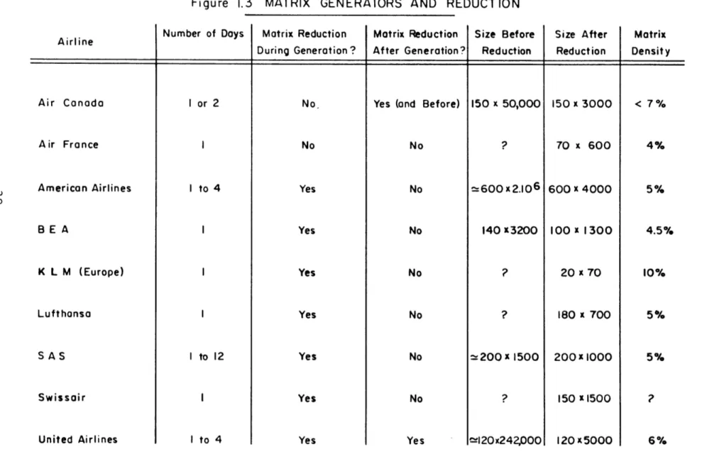
latter costs). _{The time spread of the rotation varies with} the airline; the values for several of them, as well as their respective cost structure, may be found in figure 1-3.

non-linearity of the cost. When building a rotation, one may decrease the unit cost of a partial rotation by

adding a segment: it is easy to understand this if one considers the rule guaranteeing a crew a credit of four hours of flight time per duty period. Adding a one-hour

flight to a partial rotation totaling 3 hours of flight time in the current duty period may save one hour of credit

compensation. The existence of these guarantees means that each individual rotation must be generated and costed. It is not possible to attach costs to the basic elements (segments) of the mathematical model. Instead these segments costs are generally taken as zero and only penalties caused by guarantee violations of the complete rotation are of interest as costs.

It also makes it impossible to generate rotations by increasing order of pay and credit cost although this would prove very

attractive to the OR analyst.

1.5 Rotation Matrix Reduction

When rotations are generated automatically, one may come up with more than a million acceptable rotations, ie. evidently more than any mathematical model would care to use. Some

rotations in order to make it manageable.

The next step in the crew scheduling process is to

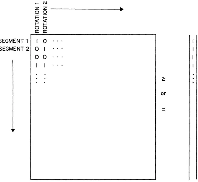
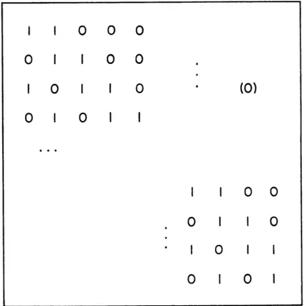
select the set of rotations of minimal total cost which cover all segments. To formulate the problem, a 0-1 matrix, A, will be used where:

A = (a..)

LJ

a.. = 1 if rotation

j

1J

= 0 otherwise

Columns are rotations and rows represent segments. Fig. 1.2 shows the type of matrix used. The matrix reduction techni-ques discussed here will reduce the size of A.

th

a. will represent the

j--

Let us define S. as

1

ie. the set of rotations

S. =

j/

S = _j/

the set of columns covering row i, including segment i:

a.= 0 = all columns - S.

1J 1

The following paragraphs describe a number of possible matrix reduction rules, R1 through R6.

i.e.

SEGMENT 1 SEGMENT 2

Ex: SEGMENT 1 is MONDAY: LOGAN - LA GUARDIA at 8!30 AM Min z cx

Ax

1

A, x BOOLEAN

1.5.1 Deadheading Allowed

The constraint requiring each segment to be covered will be expressed as: Ax> 1 where x. = 1 if the

g-h

J

rotation is chosen in the solution and 0 otherwise. 1 is a column vector of ones.

Rl: if a

C

not deteriorate when the j-- column is deleted from the matrix.

Proof: if column

j

Remarks: the cost would not be higher if costs were

exactly equal to the values in the cost vector. However, if a "deadheading cost" were accounted for, the real-life total cost would be higher if column k replaces column

j

solution, since deadheading will increase. BEA reduces the matrix size from 250 x 25000 to 250 x 3000 with Rl (See

reference 2 ).

n

R2: if (aXU .. Ua ) C ak and ck- ,the

1 n ji

optimal solution will not deteriorate when the n columns a. Ji are deleted from the matrix.

Remarks: the preceding proof and remarks are still valid. R2 shows that reduction may take place on the first

level, as in Rl, or at any higher level. The problem is that the expected number of columns which will be reduced per

second of computer time decreases very sharply as higher levels of reduction are used.

1.5.2 No Deadheading Allowed

The constraint is now Ax = 1.

R3: if S

C

S k 0 S. may be deleted without increasing the cost of the optimal

k i

solut ion.

Proof: if a column covers k and not i, it cannot be included in a feasible solution. If it were, to satisfy row ronstraint i,one of the columns of S. would have to be

selected and that would add a second '1' to row k (SkC Si)i row k's constraint could not then be satisfied any more

(since x. 0 V

j).

Row i may be deleted since it is now (after the column reduction) identical to row k; as a consequence, it is a

k in the reduced problem will implicitly satisfy row constraint i.

R4: if (S.U...JS.

)

C

li in k1 2 n

columns belonging to S S1C5.f I...AS- may be deleted

k 1 1In

without increasing the cost of the optimal solution.

Remark: _{the preceding proof applies in the same way.} Here again, one must notice that if higher levels of reduction

are used, ie. n>l, the operation becomes more costly and the benefit decreases; the benefit/cost ratio therefore

deteriorates sharply as n increases.

1.5.3 Non-optimal Reductions

It may happen that, after these reductions, there are still too many columns for the mathematical model. Reductions must then be applied which will force out enough columns to bring the size down to manageable levels in such a way that

the cost of an optimal solutions is unlikely to be increased. There are numerous heuristics which may be defined for that purpose; let us just state two of them.

tests likely to force out expensive rotations.

Example: refuse rotations for which a duty period has less than, say, four hours of flight time. Several tests

of this type may be introduced; another one would be to reject connecting times between segments of more than a certain

number of hours, since otherwise the duty time/flight time

ratio would probably be bad. This rejection rule is attractive since it stops generating and costing "bad" rotations.

R6: exclude rotations costing more than a given value if a pay and credit cost structure is used. Some segments are "bad" and all rotations including them may be costly; this rule would favor rotations containing the "nice" segments

and the matrix would not be balanced. Of course, the cost bound could be a function of the segments included. The reduction would then become more elaborate.

1.5.4 Conclusions on Reduction

One type of reduction was not discussed here, the

logical reduction. For example, when only one '1' appears in a row, the column containing it must be included in the

type of reduction is both obvious and unlikely to happen considering the large number of rotations which may be generated.

There were three classes of reduction techniques: a) a class of reduction techniques for Ax > 1 which do not increase the cost of the optimal solutions (as defined in the cost vector).

b) a class of reduction techniques for Ax = 1 which only delete infeasible columns.

c) a class of heuristic reductions which greatly (and cheaply) reject rotations (partial or complete) and may, although with a small probability, limit the problem to less-than-optimal solutions.

In each of the first two classes, a first-level and multi-level reduction technique were demonstrated. First multi-level re-ductions delete columns and rows faster and at a smaller cost

than multi-level reductions.

One must keep in mind that, in the process of generating, reducing and selecting a covering set of rotations, the analyst

should be minimizing the total cost of computation and crew schedule costs:

where CCG, CCR, and CCS are the computer costs of these generation, reduction and selection runs, and CSR is the pay and credit cost of the crew schedule.

In fact, the real problem is to minimize C over different computer methods or even manual methods. However, monthly CSR costs are generally large enough that, if computer methods save a small percentage of CSR costs, it would pay for hours of computer time. For this reason, the author is persuaded that a completely manual or even heuristic operation will not be a better answer for most airlines. For example, saving

5% of the pay and credit cost using computer methods may

represent $250,000/year.

Figure 1-3 indicates the type of problem solved by each airline, the size before reduction, the size after, ...

It was obtained from a poll of the airlines engaged or seriously interested in the use of computers for crew scheduling; the

poll was made during the summer of 1969. The author is very grateful to the airlines for their cooperation and the

Figure 1.3 MATRIX GENERATORS AND REDUCTION Airline Air Canada Air France American Airlines B E A K L M (Europe) Lufthansa S A S Swissair United Airlines Number of Days I or 2 I to 4 I to 12 I to 4 Matrix Reduction During Generation? No. No Yes Yes Yes Yes Yes Yes Yes Matrix Reduction After Generation?

Yes (and Before)

No No No No No No No Yes Size Before Reduction 150 x 50,000 Size After Reduction 150 x 3000 70 x 600 =600 x 2.106 1600 x 4000 140 x3200 a200 x 1500 ~l 20x242,000 100 x 1300 20 x 70 180 x 700 200 x 1000 150 11500 120 x5000 Matrix Density < 7 % 4% 5% 4.5% 10% 5% 5% 6%

1.6 Rotation Selection

The next step in the crew scheduling process is the problem of selecting the set of rotations which covers each

segment at the smallest total cost.

That is, a set of columns (rotations) must be selected from the rotation matrix A (see figure 1-2) which will cover each row (segments) at a total minimal cost. Each row must be covered at least once (Axyl) if deadheading is allowed, or

exactly once (Ax = 1) if it is not.

This mathematical problem is generally referred to as the set covering problem. It is here, where the largest amount of money seems to be involved, that the airlines require a good optimal solution technique. This thesis therefore has given special emphasis to solving the problem better and

faster than other computational methods have done in the past. Rotation selection is the only part of the crew scheduling process where all airlines must solve a similar mathematical problem. In other parts of the process, the differences in the contract agreements do not allow a general approach: one

cannot write a general purpose rotation generator or even one usable by a reasonable percentage of the carriers. The three

solution methods along with computational experience.

The formulation of the rotation selection described in figure 1-2 is very useful for the planner trying to find out how many crews he should have at each crew base to operate

at an optimal level at a time when he has freedom of action, e.g. when the fleet is not in operation yet. If, however, the planner is operating with an existing fleet, his crews have less mobility and adequate constraints must be included. There are two ways these constraints may be expressed.

1.6.1 Detailed Crew Base Constraints

At each base, a certain number of crews is available, each of them representing a potential number of flight hours which may be flown from the base during the rotation planning period.

The problem becomes: Min cx

such that Ax = 1, or Ax>l G xsg

x

E

where a row constraint in G is added for each crew base, the right hand side being the product of the number of crews in the base by the number of flight hours a crew may fly in the

Remarks

There are two drawbacks to using this formulation.

First, and this is of course the main objection, the problem will lose its nice 0-1 structure and therefore determinant values will blow sky-high (chapter 3 will explain how this presents a problem). Secondly, this formulation would still not involve the time at which the rotation is flown and the flight time load of rotations. A set of rotations may be accepted for a base which requires twice as many crews as

available on the first day and no crew on the second day if the planning period is two days. Or a set of rotations may be

selected requiring more crews than available to cover rotations which have little flight time and add up to less than the

available number of flight hours.

1.6.2 Daily Constraints

Let us now add a different set of constraints to the original problem: one per base per day of the rotation planning period. If there are three bases and a one week period, 21 constraints will extend the problem into:

Min cx

such that Ax = 1 or Ax>l Hx< h

where H is a 0-1 matrix. Example: Rotation # Day Day Day Day Day Day Day Day Base 1 Base 1 Base 1 Base 1 Base 2 Base 2 Base 2 Base 3 Day 7 Base 3 If rotation i runs i will have a one

zeroes otherwise. crews available at 1 2 3 4. _' 1 l1 1 1 Right hand Side h 3 3 3 3 8 8 8 5 5

from day 3 to day 5 from base

j,

The right hand side h contains the number the corresponding base.

Remarks

This type of constraint is at the same time more adequate to our method (0-1 matrix) and more realistic, in a sense. The drawback is that, contrary to what could happen with the preceding constraints, the assignments may require an acceptable number of crews to fly a higher than acceptable number of hours.

1.7 Monthly Bids (blocks)

Once the rotations have been selected for every day, or every week, of a month, they must be put together to form the monthly assignments the pilots will be offered. A set of rules limiting the ways rotations may be built into blocks is found in the contract between the pilots and the carrier-these rules vary with the airlines.

These rules guarantee rest periods and vacation periods of some number of consecutive days. The airline must also

schedule training periods for the pilots.

1.7.1 Manual Block-Building

This might be the best solution when, for example, the contract requires that a pilot receive the same weekly

assignment each week, or the same daily assignment each duty day of the block. The problem then is only to fit rest periods

and training periods in the month, together with duty periods in such a way that a crew flies the maximum number of hours allowed minus a safety measure which can be used up by delays, holding periods over airports, etc.

1.7.2 Heuristic Automatic Block-Building

A cheap and efficient way to build blocks is to create a template of good blocks, where duty periods are alternated with rest periods according to contract rules and in a manner

attractive to the crews. A program then maps the duty periods into blocks from the template in such a way that the maximum use of a crew is found, with some margin to take care of unforeseen events.

1.7.3 "Optimal" Automatic Block-Building

The payoff in this case has a smaller expected value, according to experienced airline OR analysts. Some people feel that much money may be saved by very sensitive block-building. Then, a block generator, similar to the rotation generator, could be used and an integer optimization program

run. The author doubts this will be a valid approach since the problem is more difficult to solve than the problem for

rotations (larger dimensions and more intricate rules). It

would pay off if the expected operational savings over one of the two other approaches were larger than the expected difference in their computational costs for the airline.

1.8 Reserve Crew Assignment

A number of crews must be on reserve to fly charters,

replace crews who are sick, crews who, due to delays, have reached their maximum flight time for the month or who have missed a connection.

Two costs are involved in the reserve crew operation: first, the reserve crews are paid the monthly minimum of flight time hours; if too many reserve bids are offered, the airline will have to pay flight hours which were not actually flown. If not enough appear, some flights would have to be can-celled or regular crews would have to be re-scheduled at a

high cost. It is therefore important for the airline to pro-perly organize its reserve crew scheduling.

predictable than one might be led to think. Investigations have shown that:

1.) There are cities from where crews call sick

more often than from others, even when this is prorated to the number of departures from the city;

2.) Crews happen to call sick more often on a Friday morning with a three-day rotation or on a Saturday with a

two-day rotation than on other weekdays.

An intelligent survey of field data will probably provide the scheduler with a good feel for reserve crew needs. He may then try to model the needs by simulation or regression analysis. He should develop a model which will inform him

on reserve crew needs, and adapt it to include a given level of reliability (e.g. cancel less than one flight/month because of lack of pilots).

Using such an approach, models have been developed which p rovide a better reliability with less reserve crews. This

can occur when the reserve crews may be found at, or flown in time to, the right airport rather than stay inactive where they are not needed.

1.9 Other Types of Crew Scheduling

Apart from airline crew scheduling, another area of crew scheduling presents some interesting problems, the area of transit systems. A typical difference is that, for transit systems, the penalties really appear in the block-building

(or bid-building), whereas it happened in the rotation selection problem with the airlines.

A good paper on rotating rosters was given in

Transpor-tation Science (ref. 6). It says that the sensitive area of transit crew scheduling is in packing assignments and rest periods, subject to penalties created by "bad" blocks. Making the rotations is not a problem since a crew usually remains on the same transit line for each assignment; there is

there-fore no flexibility in the rotation generation and selection phase.

Scheduling of crews of stewards and stewardesses has also been studied; it is however, not as sensitive as our problem

since there is not such an expensive penalty system in that case. The problem is mainly one of minimizing the amount of personnel needed.

CHAPTER II

ROTATION SELECTION

This chapter will present different possible formulations of the set covering problem which arises in rotation selection

and classify groups of solution methods currently used to solve it.

2.1 Formulations

2.1.1 General Set Covering Formulation

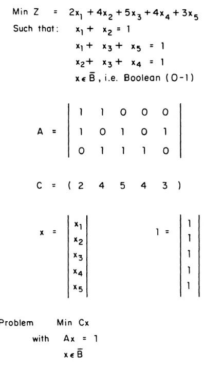
This mathematical formulation was given in the introduction. Figure 2-1 presents the set covering formulation of a test

problem to be used as an example in this thesis.

In fact, the x vector may only be required to be integer rather than 0-1. Since the cost vector is nonnegative, values greater than one will never provide a better solution than values of one.

In the description of a solution, x. = 1 when rotation

j

j

will be flown; if x. = 0, it will not be used. J

= 2x, + 4x2 +5x ₃ +4x _{4 + 3x5} Such that: xi + x2 = I x1+ x3 + X5 =1 X₂+ X₃ + X4 =1 xe B , i.e. Boolean (0-1) 1 0 0 0 0 1 0 1 1 1 1 0 C = ( 2 4 5 4 3 ) Problem Min Cx with Ax 1 xEB

Figure 2.1 SET COVERING FORMULATION OF THE TEST PROBLEM Min Z

This LP formulation is the one most used currently since good integer solutions may easily be found by manually

transforming the LP optimum.

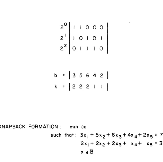
2.1.2 Knapsack Formulation for Ax = 1

An equivalent formulation results in a knapsack problem. This formulation is only applicable to the case where dead-heading is not allowed.

Let us multiply each row of the rotation matrix of A

by 2 where is is the row index. Let us define a row vector b:

b.=Z i-l

b. = . 2 a..

3 =113

Let us also define a counter row vector k:

m

k. a..

3 i= 1

which counts the number of segments each rotation has.

Theorem: there is a one-to-one correspondance between m

feasible sets Ax = 1 and (bx = 2 -1) f (kx = m) for

xE

Proof: it is clear to see that Ax = 1 will result in both bx = 2m-1 and kx = m if xE B.

20 1 1 0 0 0

2 1 0 1 0 1 2 0 1 1 1 0

b

3 5 6 4 2

k

2

2 2

I 1

KNAPSACK FORMATION: min cx

such that: 3x, + 5x 2+ 6x 3+4x 4+2x 5 = 7 2xi+ 2x2 + 2x 3+ X4+ X5 = 3

x eF

Now the reverse must be proved true. With m bits added at different positions in a binary word (since kx = m and xEB),

m m

a value of 2 -1 (since bx = 2 -1) is only obtained by putting

o . 1

one 1 in 2 , one in 2 ,...

So, the knapsack formulation will be

Min c x bx = 2m -1 kx = m

x

E

Most rotation selection problems would be too large to be solved by current knapsack codes. Figure 2-2 shows the

knapsack formulation of the test problem. The problem has been transformed into a two-dimensional knapsack

problem. It is not a knapsack problem in the traditional

sense since the constraints are equalities instead of inequal-ities. As of now, there seems to be no method which solve problems of this type with several thousand variables; in

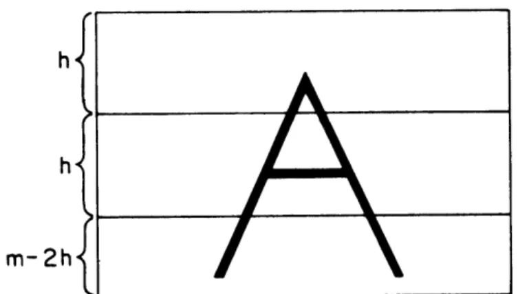
fact, even 500 variables would be too much for a fast solution. Remark: if m is large, the b.'s will be too large to

J

fit machine words. In that case, A may be divided into

h

m-2h}

Treat each row group of A as a complete matrix would be treated if m were small.

rows for which the b 's will be acceptable. Let u = mh , ie. the largest integer less than or equal to m/h. Then, vectors b1 b 2,...bu+ and k1, k2,...ku+ may be defined

as before where a horizontal block of A will play the role A played. The problem becomes:

Min c x

such that b x = 2h-1 for all k x =h I i=l,2,...,u bu+l =

m-uh-ku+1 =m-uh

xEB

The matrix structure would then be as in figure 2.3. Of course, solving a six-dimensional or an 8-dimensional knap-sack problem is much more difficult than solving a two-dimensional problem.

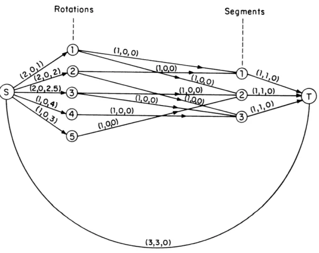
2.1.3 Network Flow Formulation

This is not an equivalent formulation of the set covering problem. It was tried by the author when he started using a branch and bound approach to solve the problem.

In the network formulation, a network consisting of a set of origin nodes connected to a main source S is linked to a set of destination nodes connected to a main sink T. The origin nodes represent rotations and the destination nodes segments. Arcs link a rotation node to all the nodes of segments included in it.

The test problem would be expressed as shown in figure 2-4 where the numbers on each arc represent the upper bound, the lower bound and the cost: (u, 1, c). The cost on each origin arc is the cost of the rotation divided by the number of segments in the rotation. Let us define:

A. = set of origins of arcs with 3 destination

j

A = set of origins of arcs with destination T

B. = set of destinations of arcs with origin _i

B = set of destinations of arcs with origin _S

K. = number of segments in rotation i

The mathematical formulation is:

Min z = c i x.

Segments

Figure 2.4 NETWORK FLOW FORMULATION OF THE TEST PROBLEM Rotations

x. = 1 (no deadheading) JT or _{x Tg} 2) x TS Sl ~ x. jT x TS 1 (deadheading allowed) SXSi 0 16B~ - x.. =0 . 13 L -

U

Vi E

B

Vj

C

B.

for

i=1,

n

Constraints (2) to (5) guarantee flow conservation at each

node. Constraints (1), (6), and (7) define upper and lower

bounds. The type of constraint in (1) shows whether dead-heading is allowed or not. If c. is the cost of rotation i, c Si may be defined as:

c . = c./K. TSi p m l i

The problem may also be formulated in a symmetrical way, subject to: 1)

with the origin nodes representing segments and the destina-tion nodes rotadestina-tions.

Remarks: This problem could be solved by direct inspection: the minimum cost solution is the solution for which: x.. = 1 for i such that:

1J

cSi = Min cSk k EA.

J

for all j=l, m

All other x values are obtained directly from the flow

conser-vation equations. Such a solution is evidently feasible and optimal.

In the network flow formulation the solution may send flow in some arcs of a rotation but not all. For this reason, some constraints should be added requiring a

capacity-or-nothing flow in each arc leading out of the main source S. Branch and bound (see section 2.2.3) should be used, but it does not converge fast enough, compared to branch and bound with LP.

2.2 Solution Methods

2.2.1 Heuristic Methods

For a long time heuristic solution methods have been used which do not guarantee optimality. Some of them are still in use where people have problems too large to solve otherwise, or when they do not know of the existence of methods good enough to solve their problem satisfactorily.

These methods obtain feasible integer solutions based on a limited search of the feasible space; to find these solutions, selection criteria are applied which "should" bring one close to an optimal integer answer.

One typical heuristic method is to solve the problem by an LP code and manually round up the non-integer values in the

solution vector to obtain a feasible integer solution, hopefully close to an optimal integer answer but quite possibly far

from optimal.

Another heuristic method would be to fix to unity the activity of all variables with unit activity in the LP

optimum: this reduction of the feasible set limits the size of the search, but again may result in a feasible solution more expensive than the optimal integer solution.

2.2.2 Implicit Enumeration

Since each of the n variables may be set to 0 or 1, there are ₂n possible solutions. This number is generally too large to find the best solution through an exhaustive

search. Implicit enumeration methods reject subsets of solutions which are known a priori not to be feasible or optimal.

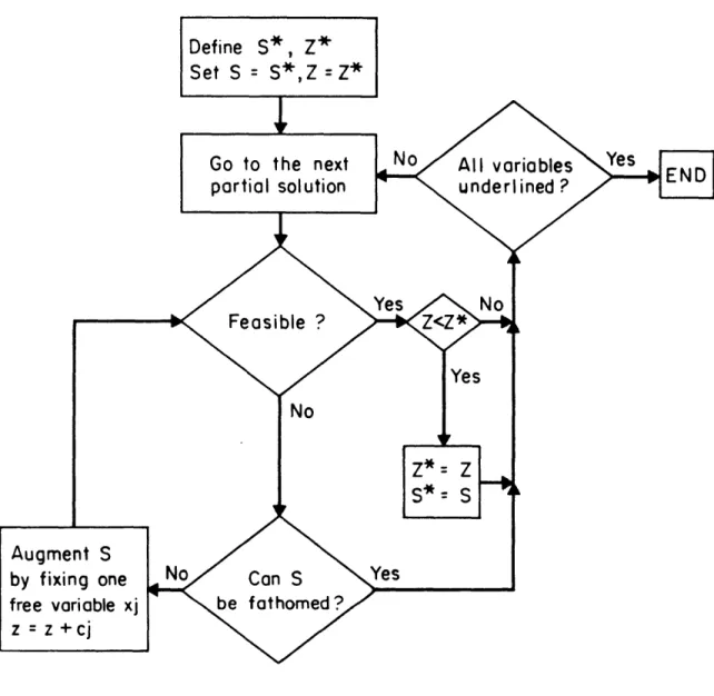
A number of elements must be defined first. We follow

Geoffrion's approach (Reference 8 ) in explaining the method. - A partial solution S is an assignment of binary

values to a subset of the n variables.

- A free variable is a variable not assigned any value by S. - A completion of a partial solution is a solution

determined by S together with a binary specification of the values of the free variables.

- A partial solution is "fathomed" if all its completions have been considered implicitly or explicitly. (S, z)

repre-sent a partial solution S and its cost z.

- Notational convention:

j

x. = 0. Example: if n = 4 (4 variables), S (3,-4,1) is a J

partial solution for which x, = 1, x₃ 1, x₄ =0 and x₂ is free. There are two possible completions: Sl = (3,-4,1,2) and S2 = (3,-4,1,-2).

A sequence of partial solutions is generated and all

their possible completions are considered. The best current feasible solution is stored together with its cost. Partial solutions are progressively completed. At each step, one of three situations arises:

a) a better feasible solution is found; it then replaces the current optimal solution S*. The next partial solution is then considered.

b) or it is clear that all completions of a

partial solution will be infeasible or more expensive than S*; go to the next partial solution.

c) or nothing can be said about S; assign a binary value to one of the free variables which therefore augments S. Test to find out whether (a), (b), or (c) is now valid.

At some point, there will be no partial solution left to be considered. All solutions will have been implicitly or explicitly covered. The optimal solution is the final S*.

The representation of S must be such that it is possible to recognize whether its other binary value has already been assigned to a given variable, the other variables being equal. For example, a variable will be underlined if the partial

solution formed by the variables preceding it in S with their current value and the variable at its other binary value

has already been fathomed. Example: S = (3,-4,1) indicates that (3,-4,-l) has already been fathomed.

The next partial solution is obtained by complementing the rightmost not underlined variable of S and dropping all elements to its right. To complement, underline the

variable and assign to it its other binary value. The next partial solution of (3,-4,1) is (3,4). It is clear that, through this procedure, the whole set of solutions has been fathomed when a partial solution has been evaluated for which all variables are underlined.

This procedure allows a complete search with a minimum of backtracking effort and table management. Computational speed is sacrificed for this advantage.

The flow chart in figure 2-5 indicates the general outline of an implicit enumeration method.

-Many different codes have been built, using different types of tests to fathom S; many different criteria have also been found for the choice of the variable which must augment S.

The author started his work on Crew Scheduling by writing and programming an implicit enumeration code (ref 22) based

on simplifications of Geoffrion's method (ref 8) allowed by the combinatorial structure of the problem. Special

Define S*, Z* Set S= S*,Z=Z* Go to the next partial solution Augment S by fixing one free variable xj z = z +cj

(S*, z*) and ordering it in an efficient way; obtaining

a good S* is important, since one may only progress sequentially from one solution to another. A good ordering is also of

major importance since the leftmost variable will stay in S very long and having fixed that variable at a "bad" level

originally will leave the method with a bad bound (z*) for most of the time; as a consequence, many solutions will be

con-sidered explicitly which would have been directly fathomed with a better bound.

Experience with this code soon indicated that for problems of the size encountered in crew scheduling the computational times would be excessive. For small problems, it seemed very fast and efficient.

2.2.3 Branch and Bound

Basically, branch and bound corresponds to first solving the LP problem without integrality constraints. If the solu-tion is integer, it is an optimal integer solusolu-tion. Otherwise, select a non-integer variable x. and solve two problems where

J

the constraints x. = 0 and x. = 1 have been added.

J J

The feasible set for the continuous problem can be partitioned into three sets, x. = 0, x. = 1 and 0 < x.<l1.

J J J

therefore does not interest us. The optimal integer solution is the minimum of the integer solutions for x. = 0 and x. = 1.

J J

A tree is built where the original node corresponds to a

continuous optimum. Each node either branches off to two nodes corresponding to opposite values of a variable not integer in its solution; or is a terminal node. At each iteration, the terminal node with the smallest solution cost is used for branching, until such a node has an integer

solution. This will be an optimal integer solution.

The author has experimented with branch and bound using LP (linear programming) and the Out-of-Kilter method(network flow formulatio as a subproblem. Convergence towards the integer optimum was much faster with the LP formulation.

The MPS (Mathematical Programming Systems) for IBM 360

was used as a subprogram by branch and bound to find the optimal integer solution to two sample problems. On the smaller

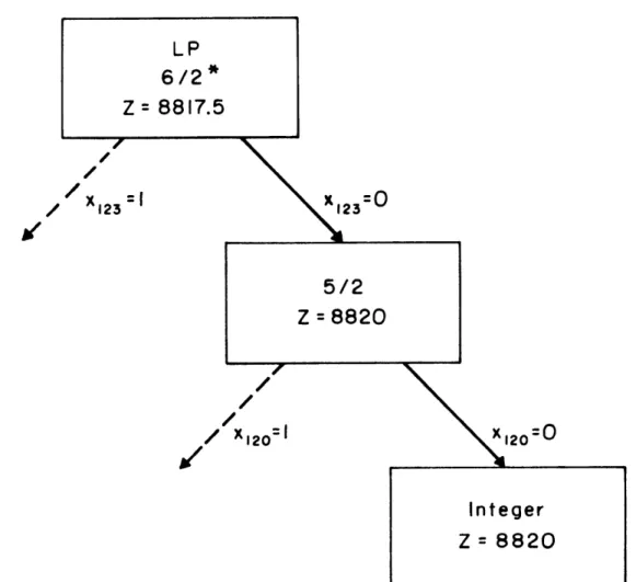
problem, 104 rows by 132 columns, the continuous optimum cost z = 8817.5. The tree in figure 2.6 is what the branch and bound process resulted in.

On the larger problem, 104 x 236, it took seven nodes and around three minutes of MPS time to obtain the optimal integer solution of 14145. Figure 4-6 on the computational results references the different problems tested during this thesis

/ 123 x123 =

X120

Figure 2.6 BRANCH AND ROUND WITH PROBLEM 5/2

Z = 8820

The column selected for branching was the non-integer column with the largest number of non-zero elements. At each level, only one branch was executed; since all column costs were multiplicands of 5 and a feasible integer solution was found at a cost of 2.5 more than the continuous optimum,

it was clear no better feasible integer solution would be found. If this had not been the case, two more nodes should have been formed.

Remarks: A number of selection criteria may be tested. The suggestions by Healy in

using values in the simplex bounds on the objective for if a variable were pushed to integer solution as a bound, variables to integer values

on the objective be greater Using this technique on the

( ref. 12) are quite interesting: tableau, one may project lower

the two branches out of a node zero or one. Using a good

it is possible to force several in one step, lest the lower bound than the good integer solution. preceding problem, the author fixed five variables to integer levels directly after running the continuous LP (before the branching); the resulting

optimum was the optimal integer solution. It took .26 min. to have the continuous optimum, .09 min. to send the relevant information from MPS to a file, .13 min. to access the FORTRAN program on file which fixed some variables to zero or one,

execute it and return, and .10 min. to obtain a new solution which was integer (and therefore optimal integer). The total

time was therefore .58 min., ie. very fast for the optimal integer solution to a 104 x 132 problem.

2.2.4 Cutting Plane Methods

The principle underlying these methods is to run a continuous linear program, add a constraint which will cut off part of the convex polyhedron of the continuous feasible set without cutting off any integer solution which could be optimal. In fact, many methods could be described as "cutting plane" which bear different names. This is pro-bably the most extensively studied area of integer programming.

The problem is first solved as a continuous linear program. If the optimal solution is not integer, a constraint is added which is a linear combination of the regular constraints from Ax > l or Ax = 1 and of some of the integrality constraints.

This process takes place until an integer solution is found to the continuous linear program. This solution is the optimal integer solution since it was obtained through an intersection of the original feasible set with some of the integrality

constraints.

found, permitting intermediate feasible solutions, it seems that, for many 0-1 problems, cutting plane methods should be

second best to only the group theoretic method; only branch and bound methods compare to cutting plane methods and some-times can provide a faster optimum.

2.2.5 Group Theoretic Method

This method will be explained in detail in the following chapter. It transforms the regular integer linear programming problem into a knapsack-type problem. The procedure is to obtain the continuous optimum and, from there, to formulate the problem as a simple one-dimensional knapsack problem whenever possible. The optimal integer solution is then

calculated through a limited search; it is so simple that in many cases, the optimal integer solution is found by direct

inspection of some output from the solution by MPS of the continuous problem.

2.3 Evaluation of the Methods

A description of the different methods the author tried

will provide some basis for evaluation. The list of the different methods is given in figure 2-7, the highest one

Ex.:

104

A A - I

x 132

25 minutes

Z =

8960

Non Optimal

Very Slow

Convergence

Figure 2.7

3 LP' s

Z=

8820

~

I minute

Z =

8820

25 seconds

PROGRESSION OF RESEARCH

being the first method experimented with, and so on. The first technique used was implicit enumeration where the

algorithm described in ( ref. 22 ) was used. The computation time was very small for small problems but seemed to increase

combinatorially with size. This is quite logical when con-sidering the way implicit enumeration operates.

The idea then occurred that branch and bound should be more efficient for crew scheduling problems; the same problem was solved optimally by branch and bound in around one minute

and group theory in 25 seconds. After 25 minutes with implicit enumeration, the best solution reached was not

optimal. Of course, better implicit enumeration codes exist although they would probably all take more than 30 seconds to reach the optimum.

CHAPTER III

GROUP THEORETIC METHOD

3.1 Introduction

This chapter will introduce the mathematical for-mulation of the group theoretic method and discuss the relations and applicability of this method to the

solu-tion of the rotasolu-tion selecsolu-tion problem.

An effort was made to present this chapter in an easily understandable manner since there are already several articles describing the group theoretic method

in a compact and mathematically elegant but not very readable manner.

The following section of this chapter derives the mathematical formulation of the problem. A small sample problem is then completely treated. A discussion of the determinant values one may expect from the continuous optimum to the crew scheduling problem follows. An explanation of the assumptions made in this thesis and of their implications conclude the chapter.

3.2 Mathematical Formulation

3.2.1 Introduction

Let us denote by B the set of Boolean values: an element, a vector or a matrix belonging to B is exclu-sively made up of O's and l's. Denote by N the set of non-negative integers.

The rotation selection problem is written in canon-ical form:

min z = cx Pl.

subject to Ax = 1 x N

where A is an mx (m+n)-dimensional matrix, A

E

V

j

1 is an m-dimensional vector of l's

It is possible to consider A (m,n)-dimensional and c and x n-dimensional. Adding a unit matrix only guaran-tees the existence of a feasible solution to Pl. Pl will be called the BLP, binary linear programming

problem. When x G N is relaxed in the BLP, we are re-duced to P2., the simple continuous linear programming