Average atomic number and electron density analysis with computerized axial tomography : experimental and computational feasibility studies

AVERAGE ATOMIC NUMBER AND ELECTRON DENSITY ANALYSIS WITH COMPUTERIZED AXIAL TOMOGRAPHY - EXPERIMENTAL AND

COMPUTATIONAL FEASIBILITY STUDIES by

DAVID BRUCE LANING

B.S., University of Wisconsin - Madison (1975)

S.M., Massachusetts Institute of Technology (1978)

SUBMITTED IN PARTIAL FULFILLMENT OF THE REQUIREMENTS FOR THE

DEGREE OF DOCTOR OF SCIENCE

at the

MASSACHUSETTS INSTITUTE OF TECHNOLOGY

)

June 1980

MASSACHUSETTS INSTITUTE OF TECHNOLOGY 1980

Signature of Author_________________________ Department (7 Nuclear Engineering June, 1980 Certified by Gordon L. Brownell Thesis Supervisor Certified by )7 David D. Lanning Thesis Supervisor Accepted by

Chairman, DdpartmenAal nm-Graduate Students C _e> rw3' _~ARCHIVEg

K2.80

AVERAGE ATOMIC NUMBER AND ELECTRON DENSITY

ANALYSIS WITH COMPUTERIZED AXIAL TOMOGRAPHY

-EXPERIMENTAL AND COMPUTATIONAL FEASIBILITY STUDIES

by

DAVID BRUCE LANING

Submitted to the Department of Nuclear Engineering

on June 19, 1980 in partial fulfillment of the requirements for the Degree of Doctor of Science

ABSTRACT

Computational and experimental studies of "tomochemistry" were performed. These studies involve the investigation of the feasibility of photoelectric + Rayleigh and Compton attenuation coefficient

imaging of a head-like target through the modification of a single-scan computerized axial tomography (CT) single-scanner. Compositional

(tomochemical) information is obtained from these images since the photoelectric + Rayleigh and the Compton attenuation coefficients of a substance are directly related to the weighted-average atomic

number and electron density of that substance respectively. Photon transport studies were performed and design models

developed to determine the x-ray tube voltage and spectral filtration

of the two incident spectra which could be used to determine the

tomochemical information with the maximum accuracy while minimizing

the dose to the patient. It was found that in the above context

alternated 120 kVp/2.16 mm Fe-filtered and 120 kVp/130 pm Ta-filtered spectra are the best when filter modulation alone is used, while 150 kVp/2.16 mm Fe-filtered and 120 kVp/130 pm Ta-filtered spectra are the best when simultaneous kVp/filtration modulation is used. For a single 10 second/fixed 120 kVp/30 mA scan with the above fil-trations the absorbed surface dose was determined to be about 1.8 Rad.

The results of the photon transport studies served as a basis for the design of the proof-of-principle experiment. A conventional CT scanner was modified to perform tomochemistry by adding a device which modulated the x-ray filtration so as to obtain the required

x-ray transmission information. Also, calibration and data

process-ing methods were developed to reconstruct photoelectric + Rayleigh and Compton attenuation coefficient images from the two spectra x-ray

Proof-of-principle experiments were performed to test the performance of the integrated tomochemistry scanner system. From experimental measurements it was found that the theoretical minimum of the statistical uncertainty of the reconstructed attenuation coefficients in the center of the image is about 0.2% for the conventional image, 7.5% for the photoelectric + Rayleigh image and 0.6% for the Compton image when measurements are averaged over. a 5mm x 5mm pixel area. It was also found that at a spatial

reso-lution of 4 mm tomochemistry measurements could accurately predict the photoelectric + Rayleigh and Compton attenuation coefficients near the edge of the image. However, it was found that due to

systematic errors of the polynomial fits at large solution thick-nes-ses the accuracy of the reconstructions were poorer in the center of the images. Finally, it was found that tomochemical measurements could be used to distinguish between material

proper-ties that normal CT do not readily image.

Thesis Supervisor: Dr. Gordon L. Brownell

Title: Professor of Nuclear Engineering

Thesis Supervisor: Dr. David D. Lanning

Professor of Nuclear Engineering

Dedication

5

Acknowledgments

I would like to thank all those people who aided in bringing

this research project to a successful completion. In particular I

would like to thank Professors Gordon L. Brownell and David D. Lanning for their advice and direction throughout this research project.

Professor Brownell was particularly effective at aiding the author in maintaining an overview of this research project and in attaining

an appreciation of the relevance of this work to the medical research

community. Conversely, Professor Lanning was highly effective at making sure that the author did not overlook the engineering details

which were crucial to the success of this research project.

I would like to thank Tim Walters, Dave Kaufman, Charlie Burnham, Dave Chesler, Joel Lazewatsky, and Wesley Akutagawa of the MGH Physics

Research Laboratory for their aid with much of the technical work in this thesis. Tim Walters deserves special mention for his invaluable insight into the mechanics of the MGH scanner software. Without his

truly professional help it would have been extremely difficult to

understand most of the peculiarities of the pre-thesis software or to develop the new software required in this project. Dave Kaufman was

also very helpful as an extra pair of skilled hands to help put the

experiment together as well as to help find the gremlins that always seem to sneak into electronics systems.

The author would also like to acknowledge the financial support of the Nuclear Engineering Department as well as the two years of

Thanks are also extended to Priscilla Kelly and Jane Patterson

for typing the manuscript and taking the time to do the job right. Priscilla Kelly deserves special mention for the excellent way in which she layed out the format of the text, formulas, tables, and figures.

Particular appreciation is expressed to Greg Greeman, Kord Smith,

Neil Novich, Mark Broussard, Mark Gottlieb, Kim Kearfott, Manzar Ashtari, Owen Deutsch, Bob Zammenhof, Sue Best, Tommy Thomas, Steve Herring, Dave Boyle and all the other students and faculty I have met at MIT for their encouragement, friendship, and camaraderie during my studies in the Nuclear Engineering Department. I will

certainly remember with fondness the student-faculty dinners, the semi-annual picnics, the post-generals parties, and all the other

'educational' experiences within the department.

I would also like to thank my parents and my brothers and

sisters for their continuing confidence and optimism throughout my

education. Also, I would like to thank my friends who went to school with me at the University of Wisconsin. In particular, I would like to thank Robert Wood, Jeff Archibald, Mike Cain, Tom Prijic, and Nick Sharrow for their continuing encouragement and friendship. To

have friends like these make me feel like a rich man.

Finally, I would like to thank my wife, Anita Sarosiek. It

was her love, friendship, understanding, patience, humor, and

affec-tion that gave me hope when there was no hope, new enthusiasm when things were going wrong, and strength when I needed it the most.

Biographical Note

The author was born in Milwaukee, Wisconsin on September 18, 1953.

He was raised in _{Milwaukee and his high school education was within} the public school system. In high school he was active in athletics, student government and other activities. In his senior year he was the gymnastics team captain and he placed second and seventh in the city and state gymnastics championships, respectively. He graduated from John Marshall High School with the highest academic honors and he was chosen as the outstanding high school athletic-scholar of 1971 by the Common Council and Mayor of the City of Milwaukee.

In _{September of 1971 he entered the University of} Wisconsin-Madison. There he was supported by a combination of state scholarships

and work-study jobs within the experimental physics research laboratories at the University. The experimental physics work included a two year term as a visiting scientist at the Fermi National Accelerator

Laboratory in _{Batavia, Illinois. Besides the commitment to academics}

the author was for two years active within the University as a

University cheerleader. In 1975 he graduated from Wisconsin Summa Cum Laude with a B.S. in Engineering Physics and Applied Mathematics.

The author entered the Massachusetts Institute of Technology in

September of 1975. He was supported for the first three semesters as a teaching assistant in _{the Nuclear Engineering Department and for} the following two years the author was the recipient of the Whitaker Health Sciences Fellowship. In June of 1978 the author received an

S.M. in Nuclear Engineering from M.I.T.

After completion of his S.M. degree the author was married to Anita Sarosiek in August of 1978.

8

Upon completion of his thesis, the author plans to work at the Oak Ridge National Laboratory in Oak Ridge, Tennessee where the

author will work within the Instrumentation and Controls Division as a Eugene Wigner Fellow.

The author is a member of the American Nuclear Society, the American Physical Society, the Institute for Electrical and Electronics Engineers, Phi. Beta Kappa, Phi Kappa Phi, and Sigma Xi.

Table of Contents Page ABSTRACT 2 DEDICATION 4 ACKNOWLEDGMENTS 5 BIOGRAPHICAL NOTE 7 LIST OF FIGURES 12 LIST OF TABLES 19 CHAPTER 1 1.0 Introduction 21

1.1 General Description of a CT Scanner 23

and Its Images

1.2 Underlying Physical Principles of, and 40

Motivation for, Composition Analysis

CT (Tomochemistry)

1.3 Methodologies Used for Tomochemical Analysis 46

1.4 Plan of Work 60

CHAPTER 2

2.0 Engineering Design of a Single Scan 65

Composition-Analysis CT Scanner

2.1 Support Work in Nuclear Engineering 67

2.lA Physical Characteristics of the MGH 68

Benchtop Scanner

2.lB Physical Models and Figures-of-Merit 81

Used in the Tomochemistry Spectra Study

2.1C Findings of the Photon Transport Studies 93 2.1D Conclusion - Findings of the Nuclear 112

Engineering Studies

2.2 Electrical and Mechanical Engineering Con- 113

siderations in the Beam Analyser Design

2.3 System Integration and Control of the 123

Tomochemistry Proof-of-Principle Scanner

2.4 Summary 142

CHAPTER 3

3.0 Software Development and Data Analysis Methods 143

3.1 Overview of the Software Required for 144

Tomochemistry ₁₅₅

3.2 Calibration Data Acquisition and Reduction

3.3 Tomochemistry Data Mapping and Data Correction 180

Page CHAPTER 4 189 190 193 206 220

4.0 Experimental Methods and Results

4.1 Brief Review of the Experimental Setup 4.2 Experimental Determination of the Optimal

kVp for Tomochemistry

4.3 Results of the Transmission Measurement

Calibration Experiment

4.4 Results of the Proof-of-Principle Experiment CHAPTER 5

5.0 Summary

5.1 Major Methods and Models Developedand Major Theoretical and Experimental Results and Conclusions

5.2 Suggestions for Future Work APPENDIX A APPENDIX B APPENDIX C 241 242 256 258 272 273 287 309 333 334 337 339 344 363 389 390 396 420 431

Image Reconstruction Theorems of Tomography Transport Models and Calculations Used in the

Nuclear Engineering Design

B.1 Solution of the Analytic Dose Kernel for Dose Received from CT Scanning

B.2 Monte Carlo Photon Transport Determination of Dose Received from CT Scanning

B.2A Listing of the Three-dimensional Monte

Carlo Photon Transport Programs - TOMODOSE B.3 Models Used in the Spectrum - Design

Code - RELSLIB3

B.3A X-ray Tube Model B.3B Filter Model

B.3C Detector Model

B.3D Water Cylinder Target and Resolution Element Model

B.3E Listing of the One-Dimensional Photon

Transport Program - RELSLIB3

Complete Listing of the Software Used in the Experimental Data Acquisition, Reconstruction, and Display

C.1 Listing of the Programs Used to Setup the

Data Files Prior to the Scan - TCSETUP C.2 Listing of the Programs Used to Spool

in the Experimental Data TSPOOL

C.3 Listing of the Data Cleanup and

Pre-processing Programs - TCNORMAL

C.4 Listing of the Data Mapping and

Tomochemistry Data Processing Programs

Page

C.5 Listing of the Calibration Data 453

Reduction Programs - REGCHVAR

C.6 Listing of the Data File Defanning 475

Program - TCNDEFAN

C.7 Listing of the Data Reconstruction 483

Programs - TCBRECON

C.8 Listing of the Reconstructed-Image 493

Display Programs - FILEDISP

GLOSSARY OF TERMS 526

LIST OF SYMBOLS 529

List of Figures

Figure No. Page

1.1.1 Illustration of the typical x-ray projection 24 radiographic method (J.1).

1.1.2 Schematic illustration of the linear 26

tomographic method (J.1).

1.1.3 Diagram of the pencil x-ray beam arrangement 28

used to measure the attenuation coefficient line integral (J.1).

1.1.4 Schematic diagram of the translate-rotate 29

scan method used in the first commercial

CT scanner.

1.1.5 Illustration of the CRT grey scale format 31

display of a reconstructed image.

1.1.6 Typical relative dimensions of a whole-body 33

CT scanner.

1.1.7 Illustration of the continuous rotation 34

method of scanning used in whole-body

CT scanners.

1.1.8 Summary of the major characteristics of 36

fan beam whole-body CT scanners.

1.1.9 Schematic diagram of the MGH benchtop CT 37

scanner.

1.2.1 Attenuation coefficients for photons in water. 42

1.3.1 Measured estimates of atomic number versus 48 density for abnormal brain tissue (D.1).

1.3.2 Illustration of beam hardening phenomenon. 51 1.3.3 Computed effective atom number versus molar 52

concentration of iodine in water for four different parameterizations of Z.

1.4.1 Schematic representation of the modification 61

of

1.4.2 Block Diagram of the tomochemistry scanner 62

Figure No. Page

2.lA.1 _{Schematic drawings of fixed and rotating 69}

anode x-ray tubes.

2.lA.2 Experimentally determined bremsstrahlung 72

x-ray spectra from an x-ray tube run at constant voltage potential (S.4).

2.lA.3 Schematic drawing of the internals of the 76

MGH detector.

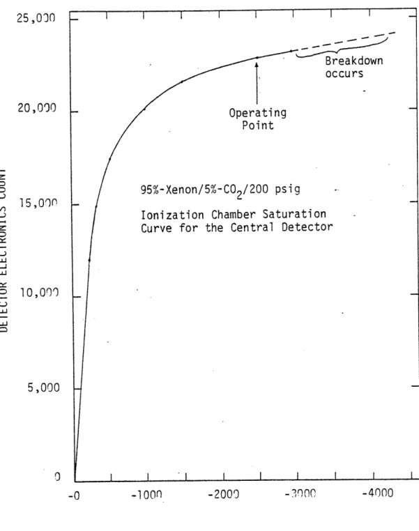
2.lA.4 Experimentally determined saturation 78

curve for the detector's central ionization chamber (#129).

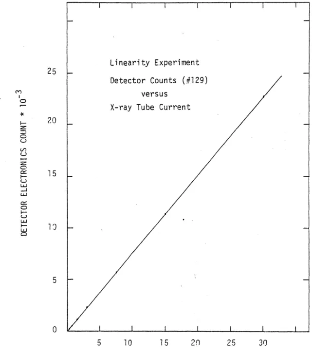
2.lA.5 Measurement of detector linearity for the 80

central ionization detector (#129).

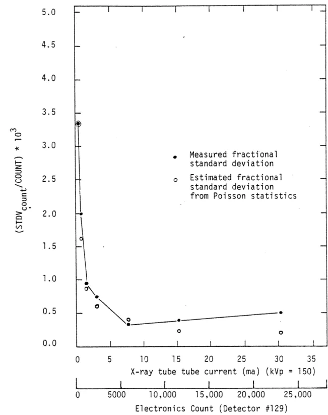
2.1B.1 Fractional standard deviation of the x-ray 83

detector current versus the x-ray tube electron beam current (or electronics count) when the tube is operating at

150 kVp.

2.1B.2 Top view of the experiment simulation model. 86

2.1C.1 Sensitivity factor versus filter atomic 94 number for a 100 kVp x-ray spectrum for

five different fractional transmissions, F.

2.1C.2 Sensitivity factor versus filter atomic number 95

for a 150 kVp x-ray spectrum for six different fractional transmissions, F.

2.1C.3 Surface dose per energy detected versus 100

fractional transmission, F, for the four different x-ray tube voltage-filtration combinations.

2.lC.4 Photoelectric + Rayleigh attenuation coef- 103

ficient statistical measurement error versus fraction transmission, F, for a 150 kVp/Fe and 150 kVp/Ta incident spectra pair.

2.1C.5 Photoelectric + Rayleigh attenuation coef- 104 ficient statistical measurement error versus

Figure No. Page

2.lC.6 Photoelectric + Rayleigh attenuation coef- 105

ficient statistical measurement error versus fractional transmission, F, for a 150 kVp/Fe and 100 kVp/Ta incident spectra pair.

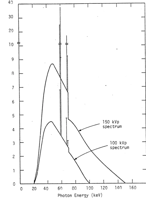
2.lC.7 X-ray spectrum distributions using x-ray 107

voltage potentials of 100 kV and 150 kV with tantalum and iron filtrations.

2.1C.8 X-ray tube flux versus x-ray tube operating 109 voltage, kV.

2.2.1 Photograph of the beam analyser disk used 114

in the proof-of-principle experiment.

2.2.2 Electrical schematic diagram of an ionization 118

chamber and its current measuring circuit.

2.2.3 Ramp model of the photon flux change to 120 account for the finite filter transition

time.

2.2.4 Response of an ionization chamber circuit 122

for six different values of ttr/RC.

2.3.1 View plan of the experimental setup. 124

2.3.2 Photograph of the operation control station. 125

2.3.3a Top view of the MGH benchtop scanner. 126

2.3.3b Rear view of the MGH benchtop scanner. 126

2.3.4 Photograph of the MGH scanner's Data 127

General Ecllipse computer.

2.3.5 Photograph of the x-ray tube used in 128 the experiment.

2.3.6 Photograph of the beam analyser disk and 130

DC motor drive in position in front of the x-ray tube.

2.3.7 Photograph of the rotating table and the 131 pulse encoder arrangement.

2.3.8 Photograph of the detector pressure vessel 132 and the A/D convertor electronics rack.

Figure No. Page

2.3.9 Method used to reject the effects of 135

transients on the measured average current.

2.3.10 Beam analyser disk position determination 136 and measurement timing method used in the

proof-of-principle experiment.

2.3.11 Ratio of the measured average iron and 138 tantalum filter currents versus filter

measurement period (inverse of the disk RPM).

2.3.12 Block diagram of the tomochemistry scanner 139 control system.

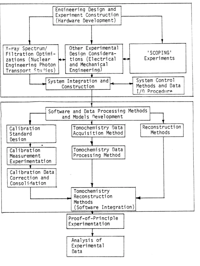
3.1.1 Block diagram of the tomochemistry data 145 processing software.

3.1.2 Schematic perspective view drawings of the 152 calibration surfaces.

3.2.1 Photograph of the four interchangeable 156 waterboxes used in the calibration

experiment.

3.2.2 Photograph of the faceplate and waterbox 157 arrangement of the calibration standard.

3.2.3 Null thickness measurement method. 161

3.2.4 Calibration standard thickness measurement 163

method.

3.2.5 Measured thickness of the calibration 164 standard waterboxes in situ versus position.

3.2.6 Illustration of the advantage of using a 166 square calibration standard.

3.2.7 Position arrangement of the calibration 167 standard on the rotating table.

3.2.8 Definition of geometry in the calibration 169 experiment.

3.2.9 Behavior of the photoelectric, Rayleigh, and 173 Compton cross sections per electron versus

Figure No. Page

3.2.10 Typical calibration data set indicating the 176

valid data range and the outliers in the data.

3.3.1 X-ray transmission through a 20 cm diameter 181

lucite cylinder (not centered on the rotating

table) versus view number.

3.3.2 Method of interpolation between measurements 182

to obtain the missing view data required for the data mapping.

3.3.3 Illustration of the linear interpolation 184 method used to obtain an estimate of the

missing view data.

3.3.4 Method of determining an estimate of the 186

contiguous measurement data sets. (Transients periods eliminated)

4.2.1 Plot of the experimentally determined values 199

of the spectrum coefficients versus kVp.

4.2.2 Calculated values of the relative uncertainty 202

of- the photoelectric + Rayleigh attenuation coefficient measurement versus the x-ray tube

kVp. (Calculations are based on experimental

measurements)

4.3.1 Percent photon transmission of the tantalum 208

and iron filtered 100 kVp spectra versus water thickness.

4.3.2 Experimental measurements of photon attenuation 209

versus solution thickness for the hard and soft spectra incident upon two different solutions.

4.3.3 Orthogonal projection drawings of the Compton 211

contour plot.

4.3.3a Detailed plot of the Compton attenuation 212

coefficient contours.

4.3.4 Orthogonal projection drawings of the 213

photoelectric contour plot.

4.3.4a Detailed plot of the photoelectric + Rayleigh 214

Figure No. Page

4.3.5 Experimental measurements of the 5.051 M 216

NaCk solution contour and of the pure water contour.

4.3.6 Plot of the measured values of the dependent 218

variables and values of the dependent variables estimated from the polynomial fit functions.

4.4.1 Reconstructions of the saline solution phantoms. 221

4.4.2 Profiles of the reconstructed values along the 222

vertical diameter of the image.

4.4.3 Display of the 0.OM NaCk and 5.0510M NaCz 225

saline solution reconstructions at a smaller display window.

4.4.4 Detailed plot of the photoelectric + Rayleigh 226

attenuation coefficient reconstruction of the

pure water solution.

4.4.5 Detailed plot of the Compton attenuation co- 227

efficient reconstruction of the pure water solution.

4.4.6 Detailed plot of the photoelectric + Rayleigh 228

attenuation coefficient reconstruction of the

5.0510M NaC solution.

4.4.7 Detailed plot of the Compton attenuation co- 229

efficient reconstruction of the 5.0510M NaCz solution.

4.4.8 Sketch of the internal structure of the 232

lucite resolution phantom.

4.4.9 Reconstructions of the spatial resolution 233 phantom.

4.4.10 Internals of the low and high contrast phantoms. 235

4.4.11 Reconstructions of the low contrast phantom. 236

4.4.12 Reconstructions of the high contrast phantom. 238

A.1 Geometry used in the image reconstruction 259

Figure No. Page

A.2 Illustration of the Nyquist-frequency- 268

limited ramp filter and its corresponding inverse Fourier transform.

A.3 Plot of the Hanning window function versus 269

spatial frequency, p.

A.4 Illustration of the Hanning-weighted ramp 270

filter and its corresponding inverse transform.

B.1.1 Geometry used in the analytic dose 274

calculation.

B.1.2 The surface dose factor versus cylinder 280

diameter for three different attenuation

coefficients, P.

B.l.3 Dose factor versus cylinder diameter at 285

different radial positions. pat 0 .2 cm~1.

B.2.1 Geometric tally regions used in the 289

Monte Carlo program.

B.2.2 Flow chart for geometry, photon interaction, 292

and energy tests in the Monte Carlo trans-port program.

B.2.3 Comparison of experimental and Monte Carlo 293

results.

B.2.4 Rad/roentgen, f, factor versus x-ray energy. 296

B.2.5 Dose per roentgen versus depth at various 299

axial heights.

B.2.6 Fraction of actual surface dose to single 301

scan dose versus axial height. (10 scans at 1 cm scan separation)

B.3D.1 Relation between the reference energy and 347

high and low energy attenuation coefficients.

B.3D.2 Picture element model used in the statistical 352

List of Tables

Table No. Page

1.1.1 Typical Physical Parameters in a CT Scanner. 38 1.3.1 Major findings of White (W.1, W.2, W.3) 53

with respect to the determination of an effective atomic number, Z.

2.1C.1 Practical engineering considerations in the 101 choice of filter materials for use in the

beam an analyser disk.

3.1.1 Data set obtained by the data acquisition 146 software. (Projection measurement only)

3.1.2 Data set obtained after taking the proper 149 ratios.

3.1.3 Data sets obtained after the line integral 153 data mapping process.

3.2.1 Measured thickness dimensions of the 158 waterboxes and measured molar

concentra-tions of the saline soluconcentra-tions.

3.2.la Errors noted to be of significance in the 160

CT scan and calibration measurement process.

3.2.2 Sequence of the saline concentration-standard 172 thickness combination in the calibration

measurements.

3.2.3 Sample output of the calibration data reduction 179 (polynomial fitting) programs.

4.2.1 Experimentally determined values of the 198

spectrum coefficients versus kVp.

4.2.2 Calculated values of the relative uncertainty 203

of the photoelectric + Rayleigh attenuation coefficient measurement versus the x-ray tube

kVp. (Calculations are based on experimental

measurements)

B.l.1 Dose factor estimates for different cylinder radii 286

and radial positions assuming yat = 0.2 cm~1

B.2.1 X-ray tube voltage-filtration combinations studied 288

Table No. Page

B.2.2 Dimensions of the annular rings used for 290

the different phantom sizes.

B.2.3 Spectrum-weighted quantities of interest 298

for data conversion and interpolation.

B.2.4 Rads per Roentgen versus average radial, <r>, 302 and axial, Z, position. 15.16 cm radius,

105 kVp, 3 mm At filtration.

B.2.5 Rads per Roentgen versus average radial, <r>, 303 and axial, Z, position. 15.16 cm radius,

105 kVp, 3 mm Az/0.2 mm Cu filtration.

B.2.6 Rads per Roentgen versus average radial, <r>, 304 and axial, Z, position. 15.16 cm radius,

105 kVp, 0.96 mm Cu filtration.

B.2.7 Rads per Roentgen versus average radial, <r>, 305

and axial, Z, position. 15.16 cm radius, 120 kVp, 3 mm At/0.2 mm Cu filtration.

B.2.8 Rads per Roentgen versus average radial, <r>, 306

and axial, Z, position. 15.16 cm radius, 140 kVp, 3 mm At/0.2 mm Cu filtration.

B.2.9 Rads per Roentgen versus average radial, <r>, 307

and axial, Z, position. 12.5 cm radius,

105 kVp, 3 mm At/0.2 mm Cu filtration.

B.2.10 Rads per Roentgen versus average radial, <r>, 308 and axial, Z, position. 18.5 cm radius,

105 kVp, 3 mm Az/0.2 mm Cu filtration.

B.30.1 Spectral characteristics of the filtered 100 kVp 361

spectrum for a range of filtration thicknesses of iron and tantalum.

B.30.2 Spectral characteristics of the filtered 150 kVp 362 spectrum for a range of filtration thicknesses

1.0 Introduction

With the development of computerized axial tomography by

Godfrey Hounsfield (H.1) a new dimension has been added to the fields

of radiology and non-destructive examination. Computerized axial tomography (CT) scanners scan thin cross sectional slices of the body

yielding two dimensional grey scale images of the spectrum averaged x-ray attenuation coefficients versus position within those slices.

CT scanning is a very accurate radiographic method with typical CT scanners capable of determining the spectrum averaged attenuation co-efficients with an error of less than 0.5% at a resolution of 1-2 mm. Within the diagnostic energy region (0-150 keV) there are three basic physical processes which cause the attenuation of photons in matter: Compton scattering, Rayleigh scattering, and photoelectric absorption. Furthermore, the magnitudes of these processes depend upon the "average" atomic number and electron density of the target being scanned as well as the energy of the incident x-rays. Hounsfield was the first to suggest (H.1) that if two different CT scans are

per-formed on the target at two different x-ray energies it is possible to obtain a grey scale image of the electron density as a function of position and another grey scale image of the "average" atomic

number. This method of obtaining composition information through the

use of computerized axial tomography is commonly referred to as tomochemi stry.

The principle objective of this thesis is to determine experi-mentally and theoretically the enqineering considerations which go

22

single scan. At this point it should be made clear. that no attempt will be made to determine the medical efficacy of tomochemistry.

The intent rather is to present the methods and results of an optimal experiment design, the new data processing methods developed, and the results of the proof-of-principle experiments. As will be seen later,

the fundamental physical assumptions, hardware design, and software methods all in some way limit the quantitative accuracy of

1.1 General Description of a CT Scanner and Its Images

Since shortly after the discovery of x-rays by Roentgen in

1895, x-rays have been used to image the internal structure of the

body. Typical radiographs are projection images of the transmission of x-rays through the body (Fig. 1.1.1). A broad beam of x-rays incident upon the patient is attenuated by the body. Some of those x-rays which are transmitted by the body are detected by a film detection medium on the opposite side of the body. The internal structure image is formed by the relative attenuation of the x-rays along different paths. Hence, in those paths where the photon attenu-ation is high, such as with the presence of bone, the radiographic

film is less exposed than in those paths where the photon attenuation is low, due to the presence of air cavities or soft tissue.

The radiographic projection method has become widely used in the medical profession because it has two advantages. The first is that film radiography can give spatial information on internal struc-tures of the body noninvasively at a relatively acceptable risk to the patient. With spatial resolutions of -.5 line pairs per millimeter

(J.1), the images are sufficiently sharp for imaging most structures of the body. The second advantage of film radiography is that radio-graphs of the patient can be made in a few seconds and then developed

in a matter of minutes so that the physician can make a diagnostic assessment of the patient rapidly and accurately.

However, in spite of projection radiography's simplicity and

ease of use, there are two main problems with the simple radiographic method. First, the x-ray projection method may mask important

rIJ

I

Fiqure 1.1.1 Illustration of the typical x-ray projection radioqraphic method (J.1).

X-ray Tube

information the physician needs for diagnosis. In particular, over-lying or underover-lying tissue may mask the desired information because the depth dimension is lost when one compresses three dimensional information into two dimensions. The second main problem of film radiography is that the photographic density of a developed image is a nonlinear function of the x-ray exposure. Thus, accurate quanti-tative radiography is difficult to perform with film systems.

To help suppress undesirable image structures the method of linear tomography was developed. In this method, as illustrated in

Fig. 1.1.2, the x-ray tube and film move simultaneously in opposite directions. This motion causes blurring of the structures to occur

in all planes except the one to be visualized. By moving the imaging sys-tem up or down one can then observe structures in different planes within the patient. Although linear tomography improves the capability of radiologists to determine spatial information, it uses a film

system; therefore quantitative radiography is still difficult to per-form with linear tomographic scanners. Furthermore, linear tomographic scanners cannot improve the radiographic situation when the soft

tissue of interest is enclosed within bone (as in the case of the brain).

In 1971 the first radiographic system which could unravel the radiographic projection information was introduced by EMI Limited: the computerized axial tomographic (CT) scanner. The original clinical

X-ray Tube Motion

Fixed Patient

Film Motion

Figure 1.1.2 Schematic illustration of the linear tomographic method (J.1).

CT scanner, invented by Godfrey Hounsfield (H.1), was intended for

head scanning only. In Hounsfield's first machine the patient was positioned within a gantry holding an x-ray tube and a single detector

as shown in Fig. 1.1.3. The scan would be performed by translating

the x-ray tube and detector past the head at a fixed gantry angle. At about 200 discrete positions along the line of the translation a pencil x-ray beam was used as a probe to measure the line integral of photon attenuation given by the expression (monochromatic source of energy E):

= exp

[

where:

yp(r,E) is the macroscopic photon cross section

(attenuation coefficient) for photons of energy E at vector position r which lies

on ray A

1/10 is the ratio of the current measured by the detector when the patient is within the x-ray beam to that current measured

with no patient in the beam

As shown in Fig. 1.1.4, after one translational measurement was completed the gantry would then be rotated by l* and the machine

It is interesting to note that Hounsfield was not the first to come

up with the idea of computerized axial tomography (D.2). However, he alone was successful in developing a clinical machine because he was able to synthesize a practical design by drawing upon the fields of mechanical and electrical engineering, computer science, and

To computer for image reconstruction Scintillation detector / X-ray tube

Fiqure 1.1.3 Diagram of the pencil x-ray beam arrangement used to measure the

attenuation coefficient line

Figure 1.1.4 Schematic diagram of the

translate-rotate scan method used in the first commercial CT scanner.

would commence another translational measurement. This process would be repeated for 180 translational measurements so that when the scan was completed the gantry would be rotated by one-half of a turn. The entire scanning process took about 5 minutes. By scanning the head

using the above method 180 sets of 200 parallel ray measurements of photon attenuation were obtained. These measurements, digitized and stored in a computer, then served as the basic data set of the

tomographic reconstruction.

The reconstruction of the image, as performed by the first scanner, was done by a matrix inversion of the basic data set. Con-ceptually, the computer reconstruction program would ask the rhetorical question: "Which two dimensional matrix of attenuation coefficients versus position would yield the set of line integrals measured in

the scan?".

* Once the two-dimensional matrix of attenuation coefficients had been determined, they were displayed on a cathode ray tube (CRT) using

a grey scale format as illustrated in Fig. 1.1.5. The reconstruction

A more common unit used by CT scanners is the Hounsfield unit which

is defined as:

(H(F)

H(r) = * 1000

Iwater where:

H(F) is the Hounsfield unit determined at pointYr

u(r) is the spectrum averaged attenuation coefficient at point r in the body for the incident spectrum used.

uwater is the spectrum averaged attenuation coefficient for water for the incident spectrum used.

Figure 1.1.5 Illustration of the CRT grey scale format display of a reconstructed image.

in Fig. 1.1.5 is that of a slice of a kitten scanned in the thoracic region. Note that one can clearly see the lung cavities, bones, and

other anatomical features. In this image a window of reconstructed attenuation coefficients is chosen for display. Those reconstructed attenuation coefficients which are less than the window minimum are displayed as black. Similarly, reconstructed attenuation coefficients greater than the window maximum are displayed as white. Those at-tenuation coefficients which lie between the window minimum and maxi-mum are displayed by linearly relating them to the grey level scale.

Since the introduction of Hounsfield's first machine in 1971, a large number of technological developments have occurred which have increased the speed, accuracy, and spatial resolution of CT scanners.

By increasing the number of detectors, using more powerful x-ray

tubes, developing faster and more sophisticated image reconstruction methods, and improving the mechanical design, 5 second scanners were developed which could scan any anatomical section of the body.

Figure 1.1.6 shows the relative dimensions of these higher generation

machines with respect to the patient.

One of the main features of these higher generation machines, as seen in Fig. 1.1.7, is the continuous rotation scan method. In this setup a collimated fan beam of x-rays is incident upon the patient. The photon attenuations within the slice being scanned are then measured by a bank of %250 detectors on the opposite side of the patient. Typically, these scanners measure about 360 views in one full revolution of the gantry. The x-ray tube used for these scanners

Figure 1.1.6 Typical relative dimensions of a whole-body CT scanner.

Fixed Patient

X-ray Tube

X-ray Fan Beam

Data to Computer

Detector Bank with %250 Detectors

Figure 1.1.7 Illustration of the continuous rotation method of scanning used in whole-body CT scanners.

because they can be run at about 100 mA electron current on the anode target at kilovoltage potentials between 100 and 150 peak kilovolts

(kVp). Furthermore, these tubes have a small (% 1 mm 2) focal spot size which is important when trying to perform high resolution radiographic

imaging. The 250 detectors, which simultaneously measure the photon transmission along the different ray paths, are either of the ioniza-tion chamber type or of the scintillaioniza-tion crystal-photon multiplier type. Both of these detector types are run in the current mode in

CT scanners due to the high photon-flux rate. These detectors are

then interfaced to a dedicated minicomputer which controls the detec-tor data input and output (I/0) and also sdetec-tores and reconstructs the measured data. With this improved design these CT scanners can scan the body in 3 t 20 seconds - depending upon the manufacturer.

Figure 1.1.8 summarizes the major characteristics of present generation

CT scanners.

Because of the highly competitive nature of CT scanner

manu-facturing, research and development of scanners is of a proprietary

nature. Hence, in an effort to bring pertinent research information into the public domain a fundamental research project was initiated at the Massachusetts General Hospital's Physics Research Laboratory. In this project a benchtop device was developed which could be used to investigate the fundamental limitations and abilities of CT

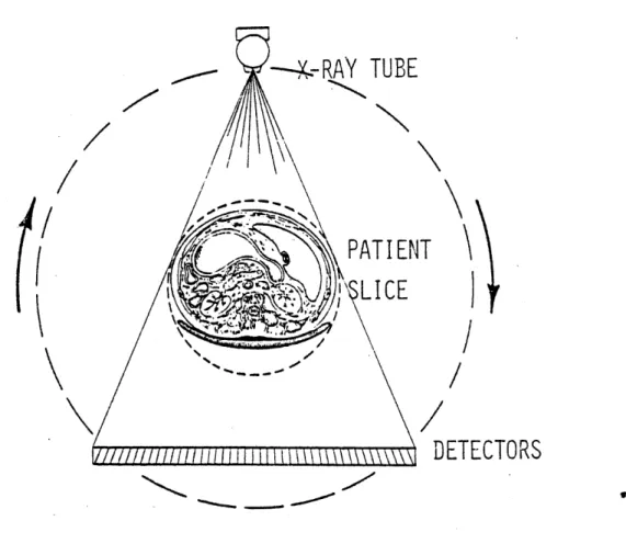
scanners. In this device, a schematic of which is given in Fig. 1.1.9, the x-ray tube and detector bank are fixed while the unknown target

of interest is rotated in 10 seconds on a rotating table. The major

----

X.-RAY

TUBE

PATIENT

LICE

DETECTORS

Key Characteristics:

Fan x-ray beam intersects a slice of the body.

256 detectors make simultaneous measurements.

X-ray tube is used due to high photon flux and point source requirements. Rotate source and detector around in 5 seconds.

Figure 1.1.8 Summary of the major characteristcs of fan beam whole-body CT scanners.

X-ray Tube

Rotating

Table Detector Bank and

Target _{Data to}

/ Computer

Figure 1.1.9 Schematic diagram of the MGH benchtop CT scanner.

.Table 1.1.1

Typical Physical Parameters in a CT Scanner

MGH X-Ray Scanner:

Scan Time

Detectors per Slice

Number of Slices Slice Thickness

Angle of Rotation

Matrix Format X-Ray Source

X-Ray Absorption Accuracy

Spatial Resolution

Data Set (No. Detectors x

No. Samples) 5 seconds 256 detectors 1 5 - 10 mm 360 degrees 320 x 320 140 kVp 0.5% 2 mm 256 x 600 = 154,000

The use of this scanner for fundamental research has two main advantages over commercial machines. First, this device is not com-mitted to a clinical schedule and therefore studies can be performed without interferring with clinical use. Second, due to the non-proprietary nature of this device, changes can be made to any part of the scanner system (hardware or software) without conflict with a manufacturer. Because of the relative ease with which hardware and

software changes could be made with this machine, all of the experi-mental and theoretical development work described in this thesis was performed with this scanner.

1.2 Underlying Physical Principles of, and Motivation for, Composition

Analysis CT (Tomochemistry)

This thesis deals with an intriguing extension of CT called tomochemistry. Tomochemistry, first mentioned by Hounsfield (H.1) and developed further by Alvarez and Macovski (A.1), refers to the analysis of CT data to obtain images of the electron density and the weighted-average elemental composition within the scanned body slice. To

understand the principle of tomochemistry, it is easiest to first consider the methodology for monochromatic photons. When a

mono-chromatic diagnostic energy (0-150 keV) photon is attenuated by matter,

it interacts with that matter in one of three ways: (1) photoelectric absorption

(2) Compton scattering (3) Rayleigh scattering.

Furthermore, it has been shown (W.1, W.2, W.3) that in a limited energy range one can express the total attenuation coefficient, total' of

biological tissue as a function of: (1) the electron density of the tissue, (2) a weighted average atomic number of the tissue, and (3) the energy of the incident monochromatic x-ray. More specifically, the

total attenuation coefficient is given by the expression (R.2):

p(E)

K E

Z-

.

_{+ aKN(E)}

₊

_{Kcoh e}

_{-20 Z-1.8}

Photoelectric Compton Rayleigh (coherent)

Absorption Scatter Scatter

where the weighted-average elemental composition, Z, is given by the expression:

Z [ pZ,4.6 / p 1/3.6

p. is the number of atoms per cc of element i

pe is the electron density in electrons per cc

E is the photon energy in keV

aKN is the Klein-Nishina cross section

K , K are constants for the photoelectric and coh coherent scattering respectively.

The basic principle of tomochemistry is that if one performs two CT scans of the body using sufficiently different monochromatic photon energies, one can uniquely determine the electron density and atomic composition profiles. As seen in Fig. 1.2.1, one would use a low energy photon beam to furnish information on the photoelectric and Rayleigh cross sections (and hence the atomic composition), and a

high energy photon beam to furnish information about the Compton cross section (and hence the electron density). By using the appropriate software one could then determine the electron density and atomic

composition profiles from the two photon measurements, and then dis-play these profiles using a grey scale format similar to normal CT scanners.

In practice polychromatic bremsstrahlung spectra are used in CT

scanners and not monochromatic photons. The complications of using polychromatic spectra for tomochemistry is one of the central problems

1.0 0.5 yTT'P+WC+yR Compton Scattering yCPea KN(E) 0. 2 0.1 Photoelectric Effect

\

Photon Energy (keV)

Fiaure 1.2.1 Attenuation coefficients for photons in water.

addressed in this thesis. The problem of polychromatic spectra is considered in the next chapter when the design of an optimal tomo-chemical scanner is considered.

There are several potential applications of tomochemistry technology which are of interest to both the medical and nonmedical

communities. A few of the medical applications are:

(1) Use the electron density information for radiation therapy

planning of high energy (n 1 MeV) photons. In a great number of hospitals in the United States and elsewhere Co6 0 is used as a radi-ation source for photon therapy. When Co60 decays it predominantly emits photons at 1.33 MeV and 1.17 MeV. At these energies the photons interact with body tissues primarily via the Compton effect. Hence, accurate (< 5% error) distributions of electron density versus

position from tomochemistry would aid in the determination of dose

distributions in a patient undergoing radiation therapy (F.1).

(2) Perform in-vivo bone mineral and bone density analysis. Efforts have been made (W.5, G.1, R.1, E.1) to use CT for bone composition analysis. The thrust of these efforts has been to distinguish be-tween, and determine the extent of, osteoporosis and osteomalacia. In _{osteoporosis there is a general decrease in the bone density (pe} decreases) during the progression of the disease, with the relative concentration of the mineral contents remaining constant. In

osteo-malacia there is a general loss of phosphorous and calcium (Z decreases)

during the progression of the disease, with the bone density remain-ing approximately constant. Radiographically or with standard CT the diseases are difficult to distinguish. However, tomochemistry can

(3) Distinguish between normal and diseased tissue. It is known (H.3) that one indicator of cancerous tissue is the presence of

calcium deposits near to, or within, the cancerous tissue. It may be possible that with tomochemical analysis one can determine whether a tissue being investigated has a higher average atomic number due to a potential tumor and the presence of calcium, or an increase in the

tissue density or.atomic number because of another pathological problem (such as the presence of a hematoma).

(4) Reduce the required concentration of contrast agents in radio-graphic contrast enhancement studies (K.1, K.2). A common technique used by radiologists is the injection into the blood stream of

iodinated compounds, commonly known as contrast agents. These agents are radiographically more opaque than soft tissue. Thus, when

radiographic procedures are performed on the patient, the blood ves-sels within the body become highly visible within the radiograph. With the use of tomochemistry it may be possible to reduce the re-quired concentration of these agents because the technique of

tomo-chemistry enhances those regions with higher average atomic number. There are a few non-medical applications of tomochemistry which may be of interest to various industries. For example, the nondestruc-tive evaluation of complicated machinery or components is one possible application of composition analysis CT. In particular, it has been mentioned (H.2) that tomochemical methods may be used for the non-destructive assay of spent fuel rods from nuclear reactors. More exactly, the determination of uranium and plutonium inventories within

45

these rods would be important for non-proliferation reasons. Hope-fully, more applications would be found with the cross fertilization of the methods developed in this thesis into other scientific and engineering areas.

1.3 Methodologies Used for Tomochemical Analysis

There are two basic methods by which the tomochemical parameters, "average" atomic number and electron density, can be determined from CT scanning. In both these methods a low energy scan and a high energy

scan are performed on the body slice of interest. However, once the

scan data is obtained, the way in which it is processed is very different. The first of the two methods, the "effective energy" - postreconstruction method, is the most widely used of the two procedures (I.1, P.3, M.4, B.1, B.2, D.1, R.2, R.3). In this method the two sets of x-ray

trans-mission data from the CT scans are reconstructed separately before

per-forming the tomochemistry data processing. One of the reconstructed

images contains the distribution of the high-energy-spectrum-averaged attenuation coefficient versus position, T(HIGH ENERGY SPECTRUM), and the other image contains the distribution of the low-energy-spectrum-averaged attenuation coefficient versus position, p(LOW ENERGY SPECTRUM). By then assuming (1) a functional dependence for the photoelectric, Compton, and Rayleigh cross sections, and also assuming (2) that the

two incident spectra can each be parameterized by an "effective energy",

once can write:

LOW - -3.28 .;3.6

-(ELOW ) K LOW P e + aKN(ELOW) e +

EFFECTIVE EFF EFF

+ K pe -2.0 Y1.8 (1.3.1)

coh Pe OW

(THIGH = K HIGH 3.6 + aKN HIGHI Pe +

EFFECTIVE EFF EFF

+ Kcoh HH0 Y -e 1.8 (1.3.2)

EFF

where:

ELOW, EHIGH are the "effective energies" of the incident

EFF EFF spectra - defined as those monochromatic

energies which have the same attenuation co-efficient for water as the spectrum-averaged attenuation coefficients measured experimentally. The other parameters are the same as in Eq. (1.2.1).

By then dividing Eq. (1.3.1) by (1.3.2) Eq. (1.3.3) is obtained. This

equation is satisfied for only one real value of Z.

p(fL) K pf -3.28-Z3.6+- ( + Kc - -2.07Z1.8

y ELOW+ PLO+KN(ELOW) ohELOW

EFF - EFF EFF EFF _(1.3.3)

-- ) KpfH -3.28-Z3.6 +I 7 K -2.071.8

y( EHIGH PHIGH + aKN(EHIGH) oh HIGH

EFF EFF EFF EFF

T can be solved in Eq. (1.3.3) by using an iterative numerical process.

Determination of pe can be made by substitution of the calculated value of Y _{into either Eqs. (1.3.1) or (1.3.2) and solving for p,.}

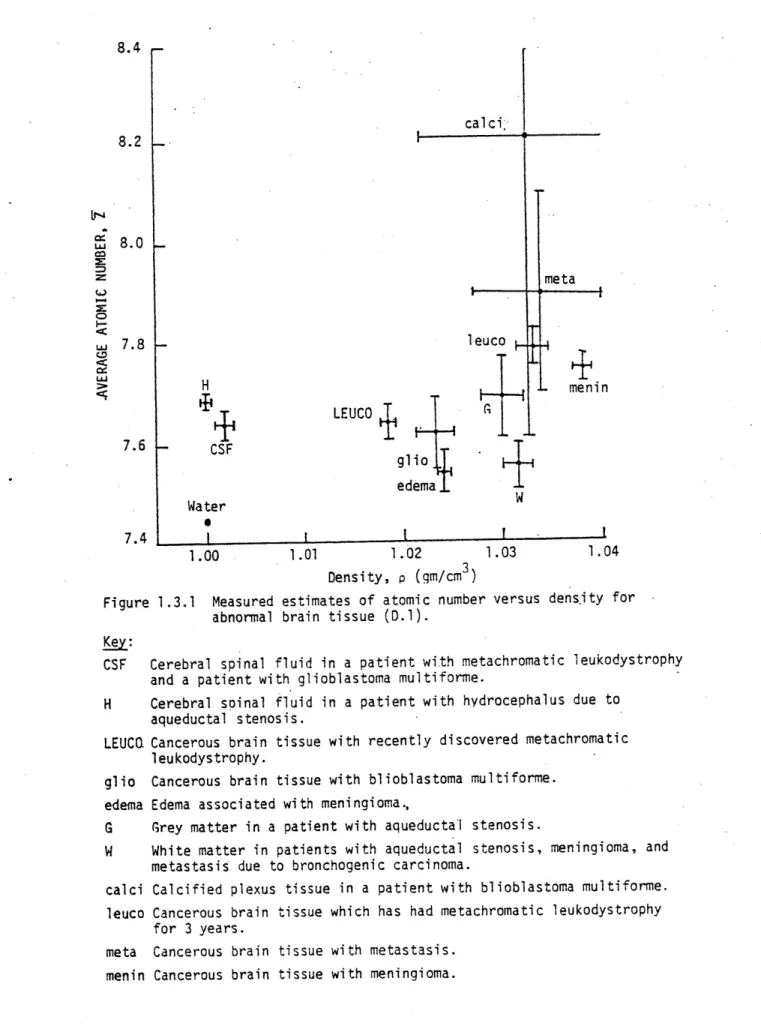
The results of an experimental clinical study (D.1) using the "effective energy" method is presented in Fig. 1.3.1. There are two main features to be noted from this figure. First, this preliminary clinical study indicates that the slight differences in soft tissue composition appear to be measurable. It is felt by this author that

8.4 calci 8.2 V-~4 U 8.0 meta 7.8 leuco H men in

'I

+

_LEUCO

Figure 1.3.1 Measured estimates of atomic number versus dens-ity for abnormal brain tissue (D.1).

Key:

CSF Cerebral spinal fluid in a patient with metachromatic leukodystrophy and a patient with glioblastoma multiforme.

H Cerebral spinal fluid in a patient with hydrocephalus due to aqueductal stenosis.

LEUC. Cancerous brain tissue with recently discovered metachromatic leukodystrophy.

glio Cancerous brain tissue with blioblastoma multiforme. edema Edema associated with meningioma.,

G Grey matter in a patient with aqueductal stenosis.

W White matter in patients with aqueductal stenosis, meningioma, and metastasis due to bronchogenic carcinoma.

calci Calcified plexus tissue in a patient with blioblastoma multiforme. leuco Cancerous brain tissue which has had metachromatic leukodystrophy

for 3 years.

meta Cancerous brain tissue with metastasis. menin Cancerous brain tissue with meningioma.

to infer more from this study - such as a pathological correlation

-would be a premature effort. The second main feature of this figure are the large error bars in the composition estimates. The large statistical error of the Z determination is due to the relatively small size of the photoelectric effect in comparison to the Compton effect. Due to dose and signal size considerations (mentioned in Chapter 2) the lower practical bound to the low "effective energy" is

about 63 keV. At this energy the ratio of photoelectric to Compton attenuation coefficients for water is about 0.075. Thus, the fractional

statistical error in the Z determination is much larger than the fractional statistical error in the p e determination.

The "effective energy" approach to tomochemical analysis is quite straightforward, however it is not rigorous. This method

suf-fers from three major types of systematic'error. First, since experi-menters rely on the reconstructions from two separate scans, they

im-plicitly assume that the patient doesn't move between scans. However, in reality this is not the case. Interscan movement of the patient can cause large errors in the determination of tomochemical parameters. The error is especially large in those regions where the tissue of interest is adjacent to a region with a very different attenuation co-efficient from the tissue being studied. In these regions a slight mismatch in positioning can cause the Z determination to diverge.

The other two downfalls of the "effective energy" method is that the Z and "effective energy" parameterization methods are too simplis-tic. Parameterizing a polychromatic bremsstrahlung spectra by a single "effective energy" is a sensitive assumption for two reasons.

First, since the photoelectric and rayleigh cross sections are strongly dependent on energy, the "effective energy" required for this theory must be known with accuracy and precision. However, no rigorous method for the "effective energy" determination of a polychromatic

spectrum exists. Second, as seen in Fig. 1.3.2 when x-ray bremsstrahlung spectra pass through the body, spectral hardening occurs; i.e., the

"effective energy" of the spectrum increases due to selective absorp-tion of low energy photons. Thus, to be truly rigorous one must determine an "effective energy" for every position within the scanned

body slice.

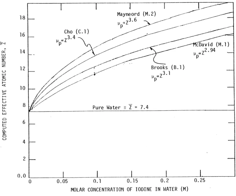
The use of one parameter,

Z,

substance. White (W.l, W.2, W.3) has performed exhaustive studies on the validity of the average atomic number concept. In general he found that linear regression fits to cross section data using a single parameter, Y, are poor in those energy regions where two Z-dependent processes are measureable. In the diagnostic energy range both Rayleigh scattering and photoelectric absorption are measureable for biological tissue; thus, White's work also puts a Z determination into question. Table 1.3.1 lists some other major findings of White per-tinent to the accuracy of tomochemical analysis.

ENERGY (KEV)

Bremsstrahlung Spectrum

100 ENERGY (KEV)

Illustration of Beam Hardening Phenomenon 200

S *1 U V U U w e

0.05 0.1 0.15 0.2

MOLAR CONCENTRATION OF IODINE IN WATER (M)

0.25

Figure 1.3.3 Computed effective atom number versus of iodine in water for four different

of Z. molar concentration parameteri zations =D L-LUi I-j Li-i_ 2 0.0

1. For photons above 10 keV in energy, the addition rule of cross sections is very accurate.

2. The Z-dependence of total cross section data has been found to give poor linear regressions, except at energies where a single process dominates.

3. The few Z-exponents published in the literature are not adequate for precise clinical radiation studies.

4. Due to the strong energy dependence of many interactions, the concept of effective atomic number based upon a single Z-exponent is not acceptable in studies attempting to characterize interactions within extended energy ranges.

Table 1.3.1 Major findings of White (W.1, W.2, W.3) with respect to the determination of an effective atomic number, Z.

The second method of data processing used for tomochemical com-position analysis is based upon the theory of Alvarez and Macovski

(A.1, A.2). As in the "effective energy" method, the required data set consists of low and high energy photon transmission measurements from a CT scanner; however, the method by which the data is processed is different. To illustrate the Alvarez and Macovski method assume for the moment that two monochromatic photon beams are used to measure photon transmissions along the same ray path in the body. As in

Eq. (1.1.1) the photon transmission equations can be written:

- n I (E1) = -(,E1)dz (1.3.4)

I(E₂)

-9n =

f(E)

)d(1.3.5)

o2 A

where

E1, E2 are the energies of the low and high energy beams

respectively.

Substituting the approximate functional form of the cross sections the line integrals can be written:

f pi(F,E )dz = f (K pe ().3.6 (-)E3.28 + K-cohe (r)1.8- E-2.0 +

A A

/. u(F,E2)dz = .8-2.0

A A (KpPeZ(r) (T)E 2 + Kcohpe(r)Z(r) +

+ P()aKN(E₂))dz (1.3.7)

where the terms in these equations are the same as in Eqs. (1.3.1) and (1.3.2).

The key to the Alvarez and Macovski method is that at this point they assume separability of the spatial and energy terms in Eqs. (1.3.6)

and (1.3.7), and they consolidate the photoelectric and Rayleigh dependences:

f ui(F,E1)dk = f aP+R(F)fP+R(El)dz + f aC(C)fC(El)dz (1.3.8)

A A A

T,

(),E2)dz = ; aP+R()f P+R(E₂)dz + / a()fC C(E₂)dz (1.3.9)

A A A

where:

aP+R(r).fP+R(E) = K P(

(

)

1.8E-2.

= photoelectric + Rayleigh cross sections

a C C(E) =p,(r)aKN(E)

Now due to separability the energy dependent terms can be taken outside of the spatial integral:

f ui(F,E1)dZ = fP+R(El) f aP+R(r)dz + fC(E1 ) f aC(F)dk (1.3.10)

A A A

f u(,E 2)dz = f p+R(E2) f aP+R(F)d + fC(E2) f aC(F)dz (1.3.11)

A A A

Hence, if the energy dependences of the photoelectric + Rayleigh and the Compton cross sections are known, Eqs. (1.3.10) and (1.3.11) can be solved for the photoelectric + Rayleigh line integral, f aP+R(r)dZ,

A

and Compton line integral, f aC(F)dz. Reconstructing the photoelectric

A

-36 K 71.8)

+ _{Rayleigh line integrals will produce an image of (peKPZ36+p Kcoh}

versus position while reconstructing the Compton line integrals will produce an image of (p e) versus position.

In practice, transmission measurements are not made with

mono-chromatic spectra. To get around the problems of spectral hardening Alvarez and Macovski considered the problem of transmission measure-ments using polychromatic source spectra. By defining:

A =fa +(r)dz

P+R A P+R

and

AC

=

aC(r)dz

the expression for the transmission ratios of two incident spectra can be written: I 1(AP+R,A) -lo I2(AP+RAc I20

f Sl(E) exp(-AP+RfP+R(E) - Ac c(E))dE

f S1(E)dE

f S2(E) exp(-AP+R fP+R(E) - A c(E))dE f S2(E)dE

Where S1 and S2 are the low and high energy- spectra used for

the transmission measurements. To then determine AP+R and Ac from these two measurements the following method was suggested: expand

1 /I and I2 2o into power series expansions:

zn(I /I g) = bo + b AP+R and zn(12 /1₂ ) = c_{0 + cIAP+R} + b2Ac + b3(AP+R)2 + bA c + c2A + c3(AP) 2 + c A 2 2 c c3 P+R c4Ac + b5 A P+RAc + c5AP+R Ac or conversely:

AP+R = B + B 1n(I1/Il) + 82n2 /12o) + B₃(zn( 1/ ₁₀))2 +

+ B₄(zn(I2 /1₂d)2 _{+ B} 5zn(I 1/Il1 )zn(12/ 20) (1.3.12) (1.3.13) and (1.3.14)