Automation and Scalability of
in
vivo Neuroscience
by
Nikita Pak
Submitted to the Department of Mechanical Engineering
in partial fulfillment of the requirements for the degree of
Doctor of Philosophy in Mechanical Engineering
at the
MASSACHUSETTS INSTITUTE OF TECHNOLOGY
June 2018
@
Massachusetts Institute of Technology 2018. All rights reserved.
Signature redacted
A uthor ...
..
...
Department of Mechanical Engineering
April 26, 2018
Signature redacted
C ertified by ...
...
Ed Boyden
Y. Eva Tan Professor in Neurotechnology
Associate Professor, MIT Media Lab and McGovern Institute,
Departments of Biological Engineering and Brain and Cognitive Sciences
Thesis Supervisor
Signature redacted
Accepted by...R
o
Rohan Abeyaratne
Chairman Department Committee on Graduate Theses
MASSACHUSETTS INSTITUTE OF TECHNOLOGY
JUN
2 52018
LIBRARIES
Automation and Scalability of in vivo Neuroscience
by
Nikita Pak
Submitted to the Department of Mechanical Engineering on April 26, 2018, in partial fulfillment of the
requirements for the degree of
Doctor of Philosophy in Mechanical Engineering
Abstract
Many in vivo neuroscience techniques are limited in terms of scale and suffer from inconsistencies because of the reliance on human operators for critical tasks. Ideally, automation would yield repeatable and reliable experimental procedures. Precision engineering would also allow us to perform more complex experiments by allowing us to take novel approaches to existing problems. Two such tasks that would see great improvement through automation and scalability are accessibility to the brain as well as neuronal activity imaging. In this thesis, I will describe the development of two novel tools that increase the precision, repeatability, and scale of in vivo neural experimentation. The first tool is a robot that automatically performs craniotomies in mice and other mammals by sending an electrical signal through a drill and measuring the voltage drop across the animal. A well-characterized increase in conductance
occurs after skull breakthrough due to the lower impedance of the meninges compared to the bone of the skull. This robot allows us access to the brain without damaging the tissue, a critical step in many neuroscience experiments. The second tool is a new type of microscope that can capture high resolution three-dimensional volumes at the speed of the camera frame rate, with isotropic resolution. This microscope is novel in that it uses two orthogonal views of the sample to create a higher resolution image than is possible with just a single view. Increased resolution will potentially allow us to record neuronal activity that we would otherwise miss because of the inability to distinguish two nearby neurons.
Thesis Supervisor: Ed Boyden
Title: Y. Eva Tan Professor in Neurotechnology
Associate Professor, MIT Media Lab and McGovern Institute, Departments of Bio-logical Engineering and Brain and Cognitive Sciences
Acknowledgments
I would first like to thank Ed for his help, inspiration, and leadership. I consider
myself fortunate to have been a member of his lab and am eternally grateful to have worked for such an amazing mentor.
I would like to thank Professor Peter So and Professor Marty Culpepper for being on my thesis committee and for their advice and guidance.
I would like to thank my parents for always supporting me and teaching me the
value of hard work, even if they ask me too many questions.
I would like to thank the entire Boyden Lab, both current and former members,
for being an amazing collection of diverse, brilliant, and dedicated people. There are too many individuals to name here specifically, and I would almost certainly forget one or two, but I want to say that you have all been great collaborators, mentors, and most importantly friends.
Contents
1 Introduction
1.1 Automated Craniotomy Robot . . . .
1.2 Dual-Objective Light-Field Microscopy . . . .
1.2.1 Description of Light-Field Microscopy . . . .
1.2.2 Obtaining Isotropic Resolution Through Combining Multiple
V iew s . . . .
2 Automated Craniotomy Robot
2.1 M otivation ... 2.2 Background ... 2.3 D esign . . . . 2.3.1 Electrical Design . . . . 2.3.2 Mechanical Design . . . 2.3.3 Derivation of Automated 2.4 Performance . . . . 2.4.1 Cranial Windows . . . . 2.4.2 Thermal Expansion . . . 2.5 Conclusions . . . . Craniotomy Algorithm
3 Dual-Objective Light-Field Microscopy
3.1 M otivation . . . . 3.2 Background . . ... ... . . . .. . . . . 3 .3 D esign . . . . 19 19 22 22 23 27 28 29 29 30 37 40 45 46 49 51 53 53 54 57
3.3.1 Mechanical Design . . . . 59 3.3.2 Image Registration . . . . 69 3.4 Perform ance . . . . 77 3.4.1 Fluorescent Beads . . . . 77 3.4.2 Larval Zebrafish . . . . 82 3.5 C onclusions . . . . 99
4 Summary and Future Work 101 4.1 Development of Tools for in vivo Neuroscience . . . . 101
4.2 Etruscan Shrew Whole Cortex Imaging . . . . 104
A Things That Didn't Work, or Could Work in the Future 109 A.1 Macro Lens Choice . . . . 109
A.2 Fixed Objective Mount . . . . 110
A.3 Making Permanent Samples . . . . 111
A.4 Tilting the Sample . . . . 112
A.5 Kinematic Couplings for Optical Parts . . . . 113
B Homogeneous Transformation Matrix Details for Automated
List of Figures
1-1 The automated craniotomy robot. . . . . 21
1-2 The dual-objective light-field microscope. . . . . 25
2-1 Diagram of electrical impedance measurement circuit. . . . . 31
2-2 Initial configuration of the automated craniotomy robot with electrical contact directly to the body of the drill. . . . . 33 2-3 Final configuration of the automated craniotomy robot with electrical
contact through a bearing with conductive grease (see Figure 2-4). . . 34 2-4 End mill and bearing with electrically conductive grease. . . . . 36 2-5 The very first craniotomies made to determine if an electrical signal can
be used to detect skull breakthrough. The inconsistent hole diameter is due to the use of a round 500 pm dental burr. . . . . 39 2-6 Normalized electric potential across the drill and mouse, as a function
of frequency, as a 500 tum dental burr is lowered into the skull for 7 different mice (step size: 10 pim for 6 mice, 50 pam for the 7th). Lower lines indicate lower drilling depth. . . . . 41
2-7 Electrical conductance across the drill and mouse, as a function of
frequency, as a 500 ,um dental burr is lowered into the skull for 7 different mice (step size: 10 ptm for 6 mice, 50 [um for the 7th). Lower lines indicate lower drilling depth. . . . . 41
2-8 (left) Normalized electric potential vs. distance traveled for 10 holes in 1 mouse skull, each represented by a different color (step size 5 pum, frequency 100 Hz). Traces were aligned (at x-axis = 0) at the point in the curve of maximum slope. (right) Same as in the right plot but converted to electrical conductance vs. distance traveled. . . . . 42
2-9 (left) Hole size, measured at the base of the skull, measured with X-ray micro-computed tomography, as a function of final normalized electric potential, with the drill stopping when various normalized electrical potentials were reached. n = 98 craniotomies in 5 mice; 200 pm drill bit (width indicated by dotted line). Each mouse is represented by a different shape, with red fill indicating visible blood related to the use of the standard pointed drill bit. For 6 of the 98 craniotomies the drill bit did not pass the bottom of the skull, and thus they are on the y =
0 line. (right) Hole size vs. electrical conductance for the data on the
left. . . . . 4 3
2-10 Automated craniotomy algorithm flowchart. . . . . 44
2-11 Representative CT scan of a skull from the experiment performed in 2-12. Scale bar 1 m m . . . . . 44
2-12 (left) Hole size as a function of final stopping normalized electric po-tential for 72 craniotomies in 3 mice with a 200 pm drill bit, step size of 5 pm, and normalized electrical potential threshold of 0.65. Each mouse is represented by a different shape. For 2 of the 72 craniotomies the drill bit did not pass the bottom of the skull, and thus they are at the y = 0 line. (right) Hole size vs. electrical conductance for the sam e data. . . . . 45
2-13 Representative CT scan of a skull from the experiment performed in
2-14 (left) Hole size as a function of final stopping normalized electric po-tential for 20 craniotomies in 5 mice with a 200 [Lm square end mill, step size of 5 pm, and normalized electrical potential threshold of 0.45. Each mouse is represented by a different shape. For 3 of the 20 cran-iotomies the drill bit did not pass the bottom of the skull, and thus they are at the y = 0 line. (right) Electrical conductance vs. hole size for the sam e data . . . . 47
2-15 Craniotomy diameter for non-machined 200 jim diameter square end
m ills. . . . . 4 7
2-16 The steps involved in creating a cranial window in a mouse skull. i:
The skull is exposed and cleaned. ii: The center point and diameter of the desired cranial window are manually chosen by the surgeon, and several holes are automatically drilled along its circumference. iii: The drill automatically interpolates between the hole locations at the appropriate depth. iv: The skull is manually removed under saline. . 48
2-17 Experimental setup with a dial indicator positioned at the end of an
end mill that had been ground flat. The end mill, drill, stereotax, and everything else was positioned exactly as it would be in a normal
automated craniotomy session. . . . . 49
2-18 Spindle length increase due to drill bearings heating up over time. . . 50
3-1 Diagram of original LFM showing how a microlens array placed in the primary image plane of the fluorescence microscope allows multiple views of the sample to be captured. Scale bar: 150 pm. . . . . 55 3-2 (left) Lateral and axial PSF of a 0.5 pm diameter bead located at
z = 28 pm off the focal plane for a 20X 0.5NA lens. Scale bar: 10 pm (center) Overlay of a larval zebrafish MIP with randomly selected spatial filters (colored dots and arrows) Scale bar: 100 pm. (right) Intensity traces of selected cells from center image. . . . . 57
3-3 Photograph of the DOLF microscope showing all of the components. Every component except for the 3 axis manipulator and sample stage is in the same location on the other arm. . . . . 60
3-4 CAD rendering of the back of the microlens holder. . . . . 62
3-5 CAD rendering of the front face of the microlens holder. . . . . 63
3-6 Microlens holder mounted in a rotation stage and translation stage,
and fixed onto a precision milled component to center it on the optical ax is. . . . . 64
3-7 Lengths of interest and design of DOLF. . . . . 64
3-8 Subset of well aligned microlens array showing small spots at the center and uniformly filled in microlenses. Scale bar: 150 pm. . . . . 67
3-9 Cumulative density function for the image registration example. . . . 70
3-10 Normalized log cross-correlation between the two arms of the DOLF. 70
3-11 Unregistered and registered projections of the volumes. . . . . 71
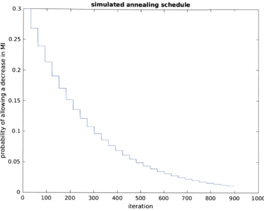
3-12 Simulated annealing schedule used in this image registration example. 72
3-13 Simulated annealing trajectory for translation in all three dimensions. 73
3-14 Simulated annealing trajectory for rotation about all three axes. . . . 74
3-15 Increase of mutual information for increasing steps of the image
regis-tration algorithm . . . . 75
3-16 Null distribution of 12,000 random registrations. . . . . 76
3-17 Fraction of null distribution that is less than the mutual information
at a given step. . . . . 77 3-18 Maximum intensity projections of the same sample taken from the two
arms of the DOLF microscope. Scale bar: 100 pm. . . . . 78
3-19 Maximum intensity projections of LFMi compared to the combined
volume. Scale bar: 100 pm . . . . . 79
3-20 FWHM for bead 1 for LFM2 and for the combined volume. . . . . 80
3-21 FWHM for bead 1 for LFM2 and for the combined volume. It is
evident in the combined view that there are two beads that could not be distinguished in the single view. . . . . 81
3-22 Plot of the z versus y FWHM in LFMI, LFM2, and the combined
volume. The line represents isotropic resolution. . . . . 81 3-23 Comparison of the volumetric reconstruction from one arm (left) and
the combined view (right). Scale bar: 50 ,im . . . . 82
3-24 Comparison of the volumetric reconstruction from the combined view (left) and a z stack from a spinning disk confocal (right). Scale bar:
50 pm... ... 83 3-25 Intensity along one line in the volume, with a moving average filter
applied. All local maxima and minima are noted. . . . . 85 3-26 Intensity along one line in the volume, without a moving average filter
applied. All local maxima and minima are noted. . . . . 85 3-27 Zoomed in section from Figure 3-25. . . . . 86 3-28 Zoomed in section from Figure 3-26. . . . . 86 3-29 Histogram of object sizes in the x axis for the single LFM reconstruction. 87 3-30 Histogram of object sizes in the x axis for the DOLF reconstruction. . 88 3-31 Histogram of object sizes in the x axis for the confocal z stack. . . . . 88 3-32 Histogram of object sizes in the y axis for the single LFM reconstruction. 89 3-33 Histogram of object sizes in the y axis for the DOLF reconstruction. 89
3-34 Histogram of object sizes in the y axis for the confocal z stack. .... 90 3-35 Histogram of object sizes in the z axis for the single LFM reconstruction. 90 3-36 Histogram of object sizes in the z axis for the DOLF reconstruction. 91 3-37 Histogram of object sizes in the z axis for the confocal z stack. .... 91 3-38 Normalized intensity along the line show for both volumes, taken from
the sam e region. . . . . 93 3-39 Normalized intensity along the line show for both volumes, taken from
the sam e region. . . . . 94 3-40 DOLF lateral resolution as the microlens array is moved away from it's
aligned location . . . . . 95
3-41 DOLF axial resolution as the microlens array is moved away from it's aligned location . . . . . 96
3-42 LFM lateral resolution as the microlens array is moved away from it's aligned location. . . . . 3-43 LFM axial resolution as t
aligned location. . . . . . 3-44 DOLF lateral resolution a
location. . . . . 3-45 DOLF axial resolution as
location. . . . . 3-46 LFM lateral resolution as
location. . . . . 3-47 LFM axial resolution as t
location. . . . .
he microlens array is moved away from it's
. .h . . . .. . .a . . . .
s the sensor is moved away from it's aligned
. . . .
the sensor is moved away from it's aligned
. . . . the sensor is moved away from it's aligned
the sensor is moved away from it's aligned
. . . .
4-1 Maximum intensity projection of a YFP mouse brain slice imaged with
the XLFM. Scale bar: 100 m. .. . . . 4-2 Maximum intensity projection of an Etruscan shrew brain slice imaged with the XLFM. Scale bar: 100 m. . . . . 4-3 Maximum intensity projection of an Etruscan shrew whole fixed brain imaged with the XLFM. Scale bar: 100 pm. . . . .
A-1 (left) Center of lens array when imaging a fluorescent slide with the
Nikon macro lens. (middle) Corner of lens array when imaging a fluo-rescent slide with the Nikon macro lens. (left) Image of random part of lens array when imaging a fluorescent slide and collimated light source with Canon macro lens. . . . . A-2 A precision machined mount to hold both objectives in the theoretically
correct position. . . . .
A-3 The original design of the DOLF microscope with one vertical arm and
one horizontal arm. . . . .
97 97 98 98 99 105 106 107 110 111 112 96
B-i Diagram of the final version of the automated craniotomy robot used in the HTM calculations. . . . . 116
List of Tables
2.1 Functional requirements for the automated craniotomy robot. .... 30
2.2 Parameters used for different tests of the automated craniotomy robot. The last row is the final, as used, configuration. . . . . 31 3.1 Functional requirements for the dual-objective light-field microscope. 59 3.2 Lateral and axial resolution of single arm LFM compared to DOLF. . 80
Chapter 1
Introduction
Many in vivo neuroscience techniques are limited in terms of scale and suffer from inconsistencies because of the reliance on human operators for critical tasks. Ideally, automation would yield repeatable and reliable experimental procedures. At the same time, precision engineering would allow us to perform more complex experiments by
allowing us to take novel approaches to existing problems. Two such tasks that
would see great improvement through automation and scalability are accessibility to the brain as well as neuronal activity imaging. In this thesis, I will describe the development of two novel tools that increase the precision, repeatability, and scale of
in vivo neural experimentation.
Chapter two describes the design, construction, and implementation of a robot to automatically perform craniotomies and large cranial windows in mammals.
Chapter three describes a microscope for imaging neuronal activity at camera frame rates with isotropic resolution in all three dimensions.
Chapter four is a short summary as well as a brief discussion of future work that links both of the projects presented here.
1.1
Automated Craniotomy Robot
Many neuroscience techniques such as electrophysiology and in vivo imaging require access to the brain. In mice and other mammals, this is achieved by manually drilling
openings through the skull, called craniotomies, to allow for probe insertion or
vi-sualization of the underlying brain tissue. Successful craniotomies require training
and skill since the skull of an adult mouse is only 150-200 pm thick. Damage to the underlying tissue while drilling can result in compromise of vasculature important for cortical maintenance [36], and release of blood can be neuromodulatory or even toxic to neurons [40, 321. Furthermore, even mild damage to the brain can reduce activity of fluorescent proteins used for functional imaging [13], in effect altering experiments that lead to our understanding of how the brain functions. Additionally, the ability to minimize the size of the craniotomy may lead to a more stable brain, which in turn should lead to longer and less noisy electrophysiological recordings.
I have developed a robot (Figure 1-1) that can automatically perform craniotomies
in mice by detecting the exact moment when the skull has been broken through
[27].
This robot relies on measuring a well-characterized increase in conductance that occurs after skull breakthrough due to the lower impedance of the meninges and cerebrospinal fluid compared to the bone of the skull. A detection circuit sends a 1 mV sinusoidal voltage through the drill bit to measure the voltage drop across the body of the mouse. Initially, this voltage drop is very high due to the large resistance of bone, but when the drill bit is through the bone, the voltage drop across the mouse decreases in a characterized manner. I created an algorithm based on this principal and built a robot that has about 5 pum step resolution in all directions to perform repeatable, precise craniotomies automatically.In my thesis, I will show how the automated craniotomy robot can create extremely precise miniature craniotomies through which probes can be inserted. Furthermore,
I will show the ability to create arrays of precise craniotomies that allow multi-shank
electrode arrays
[35]
and stimulation probes[41]
to be inserted while minimizing the amount of skull to be removed, a feature that may be very important in the stability of long-term recordings. Also, I will show the ability to create large cranial windows with the automated craniotomy robot by creating a topological map of the inner surface of the skull and interpolating between the points to mill out a precise and repeatable cranial window. In all three of these cases, the craniotomies are createdwith no damage to the brain as seen by brain bleeding.
With the ability to create precise and consistent craniotomies and cranial windows, we can improve the quality and scale of neural recordings by having a consistent means of accessing the brain without causing any damage. In the second part of my thesis, I will explore breakthroughs in one such recording technique: optical imaging of neuronal activity using fluorescent indicators.
1.2
Dual-Objective Light-Field Microscopy
1.2.1
Description of Light-Field Microscopy
Recording in vivo neuronal activity is a fundamentally difficult problem due to the high speed, small sizes, high density, and large volumes associated with the brain. Several techniques such as extracellular electrodes [31, 22, 351, patch clamping [17], and light-sheet microscopy [1] are currently used that each offer different benefits and drawbacks. Optical imaging is a promising method due to the low invasiveness, high spatial resolution, and ability to record activity from many neurons simultaneously. However, most microscopy methods can only image a single point or plane at a time, which greatly limits their usability for functional imaging of three-dimensional structures such as the brain.
Light-field microscopy (LFM) is a technique that allows for three-dimensional imaging at speeds as fast as the camera frame rate [30, 19, 4]. This is achieved by capturing both the location and the angle of the incident light using a microlens array. Capturing this 4D light-field data allows the reconstruction of a volume by using a deconvolution algorithm to solve a tomographic inverse problem. Using this microscope, we were able to capture activity data at up to 50 Hz from C. elegans, and up to 20 Hz from larval zebrafish.
While it was possible to do single cell resolution recordings of C. elegans, a lower magnification objective was used to record larval zebrafish activity because of it's larger size. This, along with the fact that there are many more neurons, packed
closer together in the larval zebrafish prevented us from capturing truly single cell activity for these recordings. In order for this technology to be more widely used, it has to be able to be used with more than just one type of organism. One of the ways of increasing the resolution of this microscope was by trying to capture more of the rays of light that come from the sample. Microscope objectives only capture a limited amount of light because they only view the sample from one side. The amount of light an individual objective lens can obtain is limited by it's numerical aperture. A (conceptually) simple way of increasing the rays of light that we capture would be to have multiple objectives image the same sample and combine the information into a single volume. This idea, applied to LFM, is the second part of this thesis.
1.2.2
Obtaining Isotropic Resolution Through Combining
Mul-tiple Views
One limitation of most optical systems is that only certain angles of light rays are cap-tured through the microscope objective. In the original LFM, this problem manifests itself as poor axial resolution in the reconstructed volume. This poor resolution makes it more difficult to extract activity data from each individual neuron, a necessary step if this technology is going to be used to replace invasive electrodes. Given that LFM already sacrifices resolution because of the trade off of spatial resolution for temporal resolution, this is an important issue to overcome. To alleviate this problem, light from more angles needs to be captured. One way of doing this is to have multiple objectives coming in at different angles around the sample to capture rays that would otherwise be lost. In the simplest formulation, two identical LFM systems positioned at 900 to each other would be able to trade off the poor axial resolution of one LFM for the relatively good lateral resolution of the other.
For the next part of my thesis, I show how a dual-objective light-field (DOLF) microscope (Figure 1-2) is able to increase the axial resolution of the original LFM without decreasing the lateral resolution or the capturing speed. Building the original LFM showed us which components are the most important in terms of getting high
quality reconstructions. These lessons influenced the design of the DOLF. Specifically, the microlens array has to be precisely aligned with the camera sensor. To do this,
I built a two degree of freedom positioner that allowed precise control of the one
translational and one rotational degree of freedom, while constraining the other four degrees of freedom. Additionally, the objective lens, tube lens, microlens array, and camera sensor must be placed in the same position on both arms of the system so that any misalignment is identical. If this was not the case, each system would
potentially image different volumes, making the reconstruction much more difficult. The two arms of the microscope must not only be aligned to each other, but both must also be aligned to the sample. Furthermore, careful thought and planning went into deciding which objectives can be used for this microscope. The magnification and NA determine the volume and resolution that can be obtained, but an additional constraint is that two objectives must be placed orthogonally to each other and still image the same volume, so the working distance has to be large enough so that they both fit. These geometrical constraints limit the number of commercially available objective lenses that can be used on this system. Finally, the DOLF must also be stable over long periods of time. This means that the proper materials and geometries must be used so there is no drift over the course of the experiment due to external forces or temperature fluctuations. All of these criteria were developed into functional requirements that were also tested on the completed microscope.
Chapter 2
Automated Craniotomy Robot
A large array of neuroscientific techniques, including in vivo electrophysiology,
imag-ing, optogenetics, lesions, and microdialysis, require access to the brain through the skull in the form of a hole in the skull called a craniotomy. Ideally, the necessary craniotomies could be performed in a repeatable and automated fashion, without damaging the underlying brain tissue. To do this, it is necessary to have a means of characterizing and detecting the moment the drill has gone through the bone of the
skull.
In my work, I discovered that when drilling through the skull a stereotypical in-crease in conductance can be observed when the drill bit passes through the skull base. I used this discovery to develop an architecture for a robotic device that can perform this algorithm. I built and characterized the performance of a robot that can automatically detect such changes and create large numbers of precise craniotomies, even in a single skull. Additionally, this technique can be adapted to automatically drill cranial windows several millimeters in diameter. This robot not only helps neuro-scientists perform both small and large craniotomies more reliably but can also create precisely aligned arrays of craniotomies with stereotaxic registration to standard brain atlases that would be difficult to drill by hand.
2.1
Motivation
Automation of craniotomies could in principle enable in vivo neuroscience experiments to be performed with greater ease, reproducibility, and throughput than is possible
by human surgeons. These benefits could in turn result in better repeatability of
experiments and higher-quality neural data, as well as the ability to deploy neural recording or stimulation probes in complex three-dimensional (3D) geometries that target multiple brain regions
[41].
Another key advantage of automating craniotomies is the ability to reduce or even eliminate any damage caused by the surgery. Bleeding can alter cortical physiology 136], and release of blood can affect neural signaling 132, 401. The precise control of drill depth presented here obviates such concerns. Additionally, the use of craniotomy robots with this skull breakthrough detection algorithm allows many small precisely spaced craniotomies to be drilled, which may be useful for deploying multi-injector
[7],
multi-electrode[22,
31, 35], or multi-optical fiber[41]
probes for interrogating distributed neural circuits. The end mills used are smaller than the commercially available burrs that are currently used for mouse craniotomies. It would be difficult for human surgeons to use such small bits.Automated craniotomies do not replace human surgeons: this method still re-quires a human to place the mouse in a stereotaxic device, expose the skull, and align the drill with appropriate structures. However, automated craniotomies should result in more consistent holes with smaller diameters and tighter spacing than previously possible. Furthermore, the opening of large cranial windows-something that typically requires extensive training-can now be performed by novice surgeons. A single exper-imenter may be able to operate multiple surgical robots in parallel. As the tools for neural recording and stimulation become increasingly sophisticated, it is important to eliminate variability in craniotomy quality as a potential failure mode for these devices. The use of conductance-based feedback is an effective way to improve the re-liability of the holes needed to expose the brain prior to inserting pipettes, electrodes, and fiber-optic cables, or for the purpose of imaging neural tissue.
2.2
Background
Automated craniotomies have been attempted before. Some methods used force feed-back or related signals to halt drill motion [20, 28], and others used an open-loop de-vice without feedback [10]. However, it is unclear whether these methods can achieve better than millimeter resolution, something that is necessary if we want to ensure that no damage to the brain or dura is to occur. Open-loop systems require CT scan-ning of the skull to measure the skull thickness, which is both expensive and involves X-rays. Still others use femtosecond lasers to ablate the skull, again, an expensive proposition
[14].
In contrast, the method presented here achieves precision in the micrometer range, and without requiring elaborate X-ray or laser technology.Early work in the Boyden Lab for automating in vivo whole cell patch-clamp neural recording
[17],
discovered that a glass micropipette being lowered into the living mouse brain underwent a stereotyped increase in pipette resistance upon encountering a cell. This enabled the ability to build a robot that could automatically patch clamp neurons in the living mammalian brain.I hypothesized that an analogous approach, lowering a drill through the skull until an increase in the conductance between the drill and the body indicated that the drill was through the skull, may be of use in automating craniotomy surgeries. This was indeed the case; a sudden increase in the electrical conductance between the drill and the body indicated when the drill was through the skull but not touching the brain.
2.3
Design
The functional requirements for the automated craniotomy robot can be seen in Table
2.1. These were determined as follows. The z resolution is based on the size of a
neuron. While neurons vary in shape and size, 5 pm is about the diameter of the smallest neurons. I wanted to be able to not damage even a single neuron. The x and y resolution are 50 pm because here, it is not necessary to be as precise as the z direction. This robot should be at least as good as human surgeons. It is hard to
Table 2.1: Functional requirements for the automated craniotomy robot.
Metric Requirement Performance
z resolution 5 pim 200 nm
x, y resolution 50 pm 200 nm
charge <1,120 nC cite 40 nC current density <0.28 A/m2 cite 0.0032 A/ 2
safety no brain bleeding no brain bleeding in >500 trials repeatability <50 pim center to center deviation 10 pm worst case standard deviation
maximum deflection <40 pim maximum 5.57 pm -due to temperature
range 10 mm x 12 mm x 5 mm 25 mm x 25 mm x 25 mm
thermal stability -40 jn expansion of spindle over 30 minutes 9 pin expansion of spindle over 30 minutes
exactly quantify how accurate human surgeons are, but I estimated that they would not be better than 1/10th the diameter of the most common (and smallest) dental burr used in mouse craniotomies. The charge and current density are determined based on the possibility of electrically stimulating the brain. These are the smallest values that could stimulate brain tissue as found in literature. The requirement of no bleeding was determined because, as described previously, bleeding can alter cortical physiology and affect neural signaling. Additionally, it is the easiest and most straightforward way of detecting damage to the underlying tissue. Repeatability is again based on 1/10th of the smallest dental burr. It would be hard for a human surgeon to be able to go back to the same craniotomy with more precision. The maximum deflection due to temperature is based on the fact that when cranial windows are made, that is the amount of skull thickness that is left behind. If there is more expansion than 40 tam, it is possible that the tool would go too far past the inner surface of the skull. The range is based on the size of a mouse brain since this was our primary focus initially. The thermal stability is also based on the 40 pm of skull that is left when making a cranial window. Typically these take about 15 minutes.
The design is split into the electrical design, mechanical design, and the derivation of the algorithm.
2.3.1
Electrical Design
The electric potential circuit works by sending a sine wave through a sense resistor and the body of the animal and finally to a measurement device (Figure 2-1).
R Sense Z Parasitics resistor DAQ Vn analog Vn Function 1/Gm= ZM Mouse input generator or DAQ
Figure 2-1: Diagram of electrical impedance measurement circuit.
Table 2.2: Parameters used for different tests of the automated craniotomy robot. The last row is the final, as used, configuration.
Electrical Sense Driving Driving Cables AC Signal Measurement V /Vmax
Contact Resistance Voltage Frequency Source Device
drill body 681 kQ 20 V 30 Hz - 100 kHz coaxial cable uenerator oscilloscope N/A
drill body 681 kQ 20 V 100 Hz twisted wires fnerator DAQ N/A
drill bit or 10 MQ 1 mV 100 Hz shielded usb DAQ DAQ 0.65 drill bit,
end mill 0.45 end mill
end mill 10 MQ 1 mV 100 Hz shielded usb DAQ DAQ 0.45
Since some initial, exploratory experiments were first performed, different combi-nations of signal sources, sense resistances, means of creating electrical contact to the animal, cables, and measurement devices were used. This information has been sum-marized in Table 2.2 for reference. When the coaxial and USB cables were used, their wire mesh shields connected to earth ground to minimize the effects of environmental noise. In all cases, the rear paw of the mouse made electrical contact to the lead of the cable connected to the measurement device through a piece of metal (contact area of
5 mm2) touching the skin of the paw and held stationary by a test clip whose spring
had been stretched to make it weaker, so as not to injure the animal. (Conductive gels may in principle facilitate this safe connectivity, but I did not find it necessary here.)
The final configuration uses an electric drill because it can accept standard 1/8 inch end mills without having to modify their diameter. The electric noise introduced from this drill was mitigated by switching the ground and signal leads so the end mill bit acts as the ground and the signal is sent through the paw.
The electric potential detection circuit relies on the ability to detect the change in the impedance across the mouse, Zm. Figure 2-1 illustrates how this circuit works. The voltage drop across the sense resistor is V, = Vi, - V., and the current flow through the sense resistor is i, = V8
/R,.
If parasitic currents, defined as ip = V,/Z,,are present, e.g., via capacitive coupling of signal wires with grounded shielding in a cable, then some of the sense current flows through a parasitic impedance Z,, calculated as the ratio V
/i,
(measured when the mouse is not there). The current flow through the mouse, when present, is im = is - ip. From these equations, the ratio of the voltage drop across the mouse to that of the input voltage, V/Vin,
is calculated asVn/Vin = 1- Rs(Zp+ Zm)/[Rs(Zp+ Zm) + ZZm]. (2.1)
When the drill tip makes a hole in the skull, it was found that Zm decreases by five orders of magnitude, and this ratio decreases by about two orders of magnitude given a sense resistance of 10 MQ.
To facilitate comparison across the multiple experimental setups initially explored, e.g., different cables and different input voltages, the voltage across the mouse, Vn, was normalized by the maximum recorded voltage, Vnmax , recorded in the open-loop
configuration with no mouse in the circuit, before drilling began. The maximum recorded voltage is equal to the input voltage, when twisted pairs are used, or less for the case of parasitic currents, which occur with the coaxial and USB cables.
In the initial experiments with the air drill, a solenoid was used to stop the supply of air to the drill and enough time was given for the drill to stop spinning before taking a measurement of the potential between the animal and the drill bit.
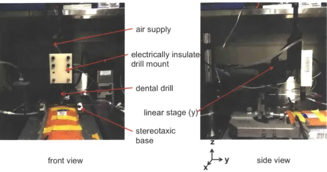
In the first iteration of the system (Figure 2-2), the impedance of the drill was included in the circuit because the simplest method for sending a signal through the drill initially appeared to be to connect a wire to the body of the drill, which is conductive to the drill bit.
air supply
electrically insulate drill
mount-dental drill linear stage (y)-stereotaxic
base z
front view y side view
Figure 2-2: Initial configuration of the automated craniotony robot with electrical contact directly to the body of the drill.
in Figure 2-1. However, in the final configuration of the robot, the impedance of the drill was removed from the circuit by attaching a bearing with electrically conductive grease to the end mill itself (Figures: 2-3, 2-4). This was done for three reasons: so that the largest potential drop across the mouse could be detected, because it was observed that the drill body impedance changed over time, and it also allows impedance measurements to be made without stopping the spinning of the bit. The impedance of the original air drill was measured as ~50 kQ new and 0.6-1.7 MQ after some wear. This is most likely due to the wear of the bearings that leads to an increase in contact resistance to the race of the bearings.
Since this method of breakthrough detection relies on sending an electrical signal through the body and brain of the animal, it is important to ensure that the maximum electrical current through the body (equal to the amplitude of the injected sine wave divided by the sense resistance) was small enough to avoid brain stimulation. A 1 mV amplitude sine wave and a 10 MQ sense resistor were chosen for the final iteration of the robot. With the cross-sectional area of a 200 pm diameter cylinder as the
three-axis
translation stage
electric hand drill
square end mill
with ball bearing
and conductive grease
stereotax
Figure 2-3: Final configuration of the automated craniotomy robot with electrical contact through a bearing with conductive grease (see Figure 2-4).
electrode area of the drill bit, the current density is ~0.0032 A/m 2
, nearly two orders
of magnitude less than the lowest current densities (0.28 A/M2
) capable of stimulating
brain tissue [5, 6, 26]. Furthermore, this current was only applied across the brain for a few seconds during the drilling operation.
The LabVIEW program that measures the impedance across the mouse does some filtering because such a low current value is used. Otherwise, it would fall below the noise threshold of the system. Initially, a simple algorithm was used. The program extracted the maximum and minimum values of 10 sinusoids, each consisting of 1,500 samples at 25 kHz, and then subtracted the minimum value from the maximum for each sinusoid and averaged these 10 differences to estimate the peak-to-peak am-plitude of the voltage drop across the mouse. For the final version, the program performed a partial discrete Fourier transform on Vs, calculating the amplitude of V, as
V,,= sqrt[Re(X)2 + Im(X)2]/N, (2.2)
where N = 15,000 is the number of samples read and X is the coefficient of the sinusoidal component of the measured samples at the test frequency (100 Hz). X is defined as
N-1
X ZXnC-i27rkn/N (2.3)
n=O
where xn is the nth measurement and k is calculated as
k = N/[sampling rate (25 kHz)/ input frequency (100 Hz)], (2.4)
which equates to the number of cycles that are recorded (in this case 60). Re(X) is calculated as
N-1
Re(X) = Y Xncos(-27rkn/N), (2.5)
n=O
and Im(X) is calculated as
N-1
Im(X) = Xsin(-2rkn/N). (2.6)
sealed ball bearing (grease removed and replaced with conductive grease)
(short) lead no diameter reduction necessary
Figure 2-4: End mill and bearing with electrically conductive grease.
The entire body of the animal is included in the breakthrough detection circuit be-cause it makes the setup much easier. There was the possibility that a more sensitive measurement could be made by decreasing the path to just around the skull. There-fore, a skull screw (self-tapping screw, size 000 thread, no. 303 stainless steel, 3/32 in. diameter) was inserted into a manually drilled craniotomy to be used as a ground electrode. No improvement was seen in the ability to detect skull breakthrough by the robot drilling at a second site, presumably because the conductance through the body and through the brain are both high compared with the conductance of the skull.
2.3.2
Mechanical Design
The system consists of a three-axis translation stage that was assembled from three linear stages, each with a linear servo motor. These motors have a repeatable step size of 200 nm and a travel distance of 25 mm and are driven with LabVIEW commands. The stages have <250 prad angular deviation which results in a maximum linear displacement of <100 nm over the thickness of the skull. A step size of 5 Am is used because that is on the order of a cell body and it was found that a smaller step size did not result in better craniotomies. Therefore, the motor and stage precision available is more than needed. Cheaper, less precise motors could easily be used if this was turned into a commercial product.
A model was used to estimate the deflection due to the forces present while drilling.
Details of this model are presented in B. The maximum force in the vertical direction was determined based on the step size used and the stiffness of the mouse skull. For a 5 pm step, and a skull stiffness of 1,500 pN/250 nm
[23],
the force in the positive z direction is 30 mN. A homogeneous transformation matrix (HTM) was used to get displacement values for the tip of the end mill based on this force. The resulting deflection is -3.4 pm in the y direction, and 59 pm in the z direction, well within the specifications. This model and HTM were also used to estimate the deflection due to thermal expansion. Before building the robot, a conservative estimate of5YC temperature rise due to things like friction from cutting, ambient temperature
changes, body heat from the animal, and heat from the heat pad the animal is on was used to get a sense of the possible deflections. This temperature rise results in a deflection of about 11.1 pm in the z direction. Later, a thermocouple was used at the drilling site to ensure that the brain is not damaged from heat as well. A 3 mm cranial window was created, and a thermocouple was introduced through this window, beneath the skull. Four holes were drilled automatically, moving the tip of the probe each time to ensure that it was directly below each hole. The maximum temperature rise directly below the end mill was measured to be 2.50C. This would result in half
However, this is a very local temperature rise and does not cause any significant deflections. Additionally, measurements were made for the thermal expansion due to the bearings in the drill heating up with use. This is explained in detail in 2.4.2.
For the original design that used an air drill, a common lab air supply was used to power the dental drill, and a solenoid valve (EV-2-6; Clippard, Cincinnati, OH) was connected between the air supply and the dental drill so that the dental drill could be turned on and off through a digital signal from the same LabVIEW program. Dental drills are inexpensive and capable of extremely high rotary rates with minimal vibra-tion, which is why they are popular in neuroscience for making small craniotomies. Most dental drills have a standard opening of 1/16 in. that fits commercially available dental burrs. These burrs range in size and shape but are only available down to 500 pm in diameter. Commercially available drill bits are very inexpensive and come in sizes of 200 pm diameter and less but have a 1 mm diameter shank that is too small to fit into the dental drill. I machined adapters that bridged this 1 mm to 1/16 in. gap in order to use these drill bits. To produce these adapters, a lathe was used to first drill a 1 mm hole in a 1/4 in. diameter aluminum rod. Next, this rod was turned down with the lathe to an outer diameter of 1/16 in. and cut to 25 mm in length. The drill bits were then cut down to ~10 mm in length with a grinding tool, and the drill bit was then press fit into the adapter. One idea that was explored was a custom made chuck that would allow various diameter drill bits to be used with the dental drill. This was abandoned because I found that the high speed of the dental drill (up to a nominal 320,000 rpm) requires a precisely balanced chuck to eliminate vibrations. The adapters are, in contrast, quite inexpensive (a few cents of material cost per adapter) and quick to produce (~15 min each). In the final iteration of the robot, the dental drill was replaced with an electric hand held drill that has accepts standard 1/8 in bits. This allows the ability to use commercially available end mills without having to modify their diameter, ensuring the best possible concentricity.
The drill bits used in initial testing have a diameter of 200 pm and a point angle of
1180. This angled cutting edge means that for a fully bored hole in the skull the drill
<A
Figure 2-5: The very first craniotomies made to determine if an electrical signal can be used to detect skull breakthrough. The inconsistent hole diameter is due to the use of a round 500 pm dental burr.
of damage. This is an issue with all pointed drill bits used in neuroscience, not just those being used with dental drills. Similarly, the round burrs must protrude ~100 pm beyond the inner surface of the skull for a fully bored-out 500 pm craniotomy. The round profile also results in inconsistent craniotomy size, as seen in Figure
2-5. Miniature square end mills (Harvey Tool, Rowley, MA) are not typically used
in neuroscience applications, even though they should result in the best possible craniotomies. This is mostly due to the prevalent use of dental drills with a 1/16 in. opening. When the dental drill was still being used, end mills with a 200 pm diameter and a 1/8 in. shank diameter were turned down by a machine shop (Contour360, Cornish, ME) to be able to fit into the 1/16 in. dental drill opening. As stated earlier, this is not necessary anymore because of the use of an electric hand held drill. Since square end mills have a flat bottom, a fully bored-out craniotomy is created when the circuit detects breakthrough of the skull. For the same reason, these are potentially less damaging to the brain as well: since they are not pointed, they do not need to extend beyond the base of the skull to complete a full craniotomy. End mills also allow for cutting in all three directions, so more elaborate craniotomies can be created.
2.3.3
Derivation of Automated Craniotomy Algorithm
Initial experiments with a dental drill mounted on a vertical translation stage showed that when the drill tip came in contact with the skull surface the observed electrical current across the body was negligible, because of the small conductance of the skull
(<0.10 nS; measured with an LCR meter, 4263B, Agilent, Santa Clara, CA). However,
when the drill tip penetrated the skull the conductance between the drill bit and the body dramatically increased because of the high conductivity of cerebrospinal fluid. To find the frequency of voltage applied that resulted in the largest electric potential drop, various sinusoidal test signals were delivered to the drill and the voltage amplitude and phase angle across the mouse was measured as a 500 pm diameter dental burr was lowered through the skull.
1.0
004
1 2 3 4 51 3 4 51 2 3 4 51 2 3 4 5 4 1 2 3 4 $ 4 5
Frequency (log Hz) Frequency (log Hz) Frequency (log Hz) Frequency (log Hz) Frequency (log Hz) Frequency (log Hz) Frequency (log Hz)
Figure 2-6: Normalized electric potential across the drill and mouse, as a function of frequency, as a 500 pm dental burr is lowered into the skull for 7 different mice (step size: 10 pm for 6 mice, 50 pm for the 7th). Lower lines indicate lower drilling depth.
15-:10~
2
0-1 2 3 4 5 1 2 3 4 5 1 2 3 4 5 1 2 3 4 5 1 2 3 4 5 1 2 3 4 5 1 2 3 4 5 Frequency (log Hz) Frequency (log Hz) Frequency (log Hz) Frequency (log Hz) Frequency (log Hz) Frequency (log Hz) Frequency (log Hz)
Figure 2-7: Electrical conductance across the drill and mouse, as a function of fre-quency, as a 500 pm dental burr is lowered into the skull for 7 different mice (step size: 10 pm for 6 mice, 50 pm for the 7th). Lower lines indicate lower drilling depth.
range of frequencies from 30 Hz to 1 kHz (n = 7 mice; Figure 2-6, voltage data; Figure
2-7, calculated conductance data). On the basis of these data, I chose a frequency of
100Hz because it showed a large electric potential drop as the drill bit passed through the skull.
Having determined that 100 Hz sinusoidal voltage was sufficient to detect skull penetration, I next sought to determine whether I could characterize the conductance as a function of drill depth in order to find a clear threshold that indicated when to stop drilling. To do that, I examined the time course of the conductance changes as the drill advanced through the skull (Figure 2-8; n = 10 holes in 1 mouse skull). It can be seen that (for each craniotomy) conductance is near zero for most of the drilling process, then jumps significantly to a higher value over a small number of steps, and then remains high for subsequent steps of the drill. This indicated that conductance does not vary appreciably as the skull is thinned but instead rises suddenly when the drill passes slightly through the inner surface of the skull.
1.0 15- 0.8- l1o-0.6 -E > 0.4 0 5-0.2 300 250 200 150 100 50 0 -50- 300 250 200 150 100 50 0 -50 Distance (pm) Distance (pm)
Figure 2-8: (left) Normalized electric potential vs. distance traveled for 10 holes in
1 mouse skull, each represented by a different color (step size 5 pm, frequency 100
Hz). Traces were aligned (at x-axis = 0) at the point in the curve of maximum slope. (right) Same as in the right plot but converted to electrical conductance vs. distance traveled.
be derived, so that the robot would stop when it completed the craniotomy without damaging the brain. The robot was operated with a 200 pm drill bit, stopping the drilling when various electrical potentials were achieved (Figure 2-9). For each trial, the diameter at the base of the skull was measured with the CT scanner. As the normalized electrical potential threshold was lowered systematically (from ~0.95 to
~0.3), the hole diameters increased, from under 150 pm to around 200 pm (n = 98
craniotomies in 5 mice). The electric potential and hole diameter were inversely cor-related (Figure 2-9, correlation coefficient r = -0.61, P = 1.26 x 10⁻⁷), with lower potential being associated with larger hole diameters. In 6 of the 98 cases, the exper-iment was stopped because of hitting a blood vessel in the skull-a benign, occasional event that yielded zero-diameter holes. In a small minority of cases, the drill suc-cessfully created a craniotomy but produced bleeding, suggesting that the standard use of a pointed drill bit yields a sub-optimal craniotomy (red symbols, Figure 2-9). I chose a threshold for the drill high enough so that bleeding could be avoided but small enough to maximize hole size. For the particular 200 Am diameter drill bits that were used in these experiments, I found that a normalized electric potential threshold value of 0.65 yielded a good balance. Later, it was found that a lower threshold of
- drill h t sdzerll t ize i 200 - 200 -A A~ *4CAA A 150- 150 -.0 .2 .4 60.) 0 ) 01
Fure 2-:(etCoesieoesrda th AoftekumasrdwhX-y
.00 M 100- * 100-S50 50-E E 6 0 i 0 0 0.0 0.2 0.4 0.6 0.8 1.0 0 1 2 3 /G, G(pS)
Figure 2-9: (left) Hole size, measured at the base of the skull, measured with X-ray micro-computed tomography, as a function of final normalized electric potential, with the drill stopping when various normalized electrical potentials were reached. n = 98 craniotomies in 5 mice; 200 pm drill bit (width indicated by dotted line). Each mouse is represented by a different shape, with red fill indicating visible blood related to the use of the standard pointed drill bit. For 6 of the 98 craniotomies the drill bit did not pass the bottom of the skull, and thus they are on the y = 0 line. (right) Hole size vs. electrical conductance for the data on the left.
0.45 worked better for the square end mills because the drill needed to go a few extra steps to ensure that the craniotomy was created.
Once it was discovered that a threshold could be defined that balanced craniotomy success and safety, I implemented an algorithm to perform electric potential measure-ments over time while a drill was lowered through the skull in 5 Am steps, halting motion when the drill-to-body potential dropped below the threshold (Figure 2-10). Across many trials of the craniotomy robot and algorithm, I found that craniotomies could be reliably drilled (Figure 2-11) with the normalized electric potential thresh-old of 0.65 derived above (Figure 2-12; n = 72 craniotomies in 3 mice). For six of the craniotomies, minor bleeding was observed from the skull after drilling to only a shallow depth (implying that a blood vessel in the skull had been hit). For four of these cases, waiting a minute or so for the blood to clot was sufficient to allow the procedure to continue to the point of a complete craniotomy at a later time. Waiting and redrilling the remaining two craniotomies was not attempted and might have allowed the successful creation of craniotomies in those locations as well.
move drill i to starting
H
position move tto x(i), y(i),( z(x(i),y(i))/measure
VrL/n maxr threshold? no dPm O yes irmnretract drill, i >N? no gyes KEY TsSdrill position to home Meaureen
Figure 2-10: Automated craniotomy algorithm flowchart.
Figure 2-11: Representative CT scan of a skull from the experiment performed in 2-12. Scale bar 1 mm.
dlrill hit size =Ldill hit "1,7e 1200 - 100-(150- 150 M Co 100 100 2 02 r - 50- 50-E E Co 0 e . . M.* 0~ 0 0.0 0.2 0.4 0.6 0.8 1.0 0 2 4 68 Vn V a Gm(JS)
Figure 2-12: (left) Hole size as a function of final stopping normalized electric potential for 72 craniotomies in 3 mice with a 200 ptm drill bit, step size of 5 Mum, and normalized electrical potential threshold of 0.65. Each mouse is represented by a different shape. For 2 of the 72 craniotomies the drill bit did not pass the bottom of the skull, and thus they are at the y = 0 line. (right) Hole size vs. electrical conductance for the same data.
2.4
Performance
Having derived and validated the automated craniotomy algorithm, the next step was to set out to see whether it was possible to develop a practical robot that could drill essentially perfect craniotomies. In addition, the holes drilled in Figure 2-12, were typically less than the width of the drill bit, because the pointed tip would break through before the wider shaft, resulting in a not completely bored-out hole. As noted above, the use of a pointed or rounded drill bit, although popular in neuroscience, may also result in part of the drill projecting significantly below the skull base, potentially injuring the brain. The final implementation of the robot uses square end mills of 200 ,im diameter and changed the threshold used to a lower value, 0.45, derived from the threshold evaluation plots (Figure 2-9). This allowed truly cylindrical holes (Figure
2-13) to be made, with diameters equal to or larger than the end mill diameter (n =
20 craniotomies in 5 mice; Figure 2-14). For 3 of the 20 craniotomies, skull bleeding was observed; in principle these could have been allowed to continue as in Figure 2-12, after a brief waiting period to allow clotting. Craniotomy sizes of >200 pm were due to some end mills not being perfectly concentrically machined down in the