Automatic tool path generation for multi-axis machining

7 /

Automatic tool path generation for multi-axis machining

by

Laxmiprasad Putta

B. Tech., Mechanical Engineering (1996)

Indian Institute of Technology, Madras.

Submitted to the Department of Mechanical Engineering

in partial fulfillment of the requirements for the degree of

Master of Science in Mechanical Engineering

at the

MASSACHUSETTS INSTITUTE OF TECHNOLOGY

June 1998

© Massachusetts Institute of Technology, 1998. All Rights Reserved.

Author ...

Department of Mechanical Engineering

May 8, 1998

C ertified by ...

Sanjay E. Sarma Assistant Professor of Mechanical Engineering Thesis Supervisor

Accepted by ...

Prof. Ain A. Sonin Chairman, Department Committee on Graduate Students

A

Ir

41998

Automatic tool path generation for multi-axis machining

by

Laxmiprasad Putta

Submitted to the Department of Mechanical Engineering on May 7, 1998, in partial fulfillment of the requirements for the degree of

Master of Science in Mechanical Engineering

Abstract

We present a novel approach to CAD/CAM integration for multi-axis machining. Instead of redefining the workpiece in terms of machining features, we generate tool paths directly by analyzing the accessibility of the surface of the part. This eliminates the problem of

feature extraction. We envision this as the core strategy of a new direct and seamless CAD/ CAM system. We perform the accessibility analysis in two stages. First, we triangulate the surface of the workpiece and perform a visibility analysis from a discrete set of orienta-tions arranged on the Gaussian Sphere. This analysis is performed in object space to ensure reliability. For each triangle, a discrete set approximation of the accessibility cone is then constructed. Next, a minimum set cover algorithm like the Quine-McCluskey Algorithm is used to select the minimum set of orientations from which the entire work-piece can be accessed. These set of orientations correspond to the setups in the machining plan, and also dictate the orientation in which the designed part will be embedded in the

stock. In particular, we bias the search for setups in favor of directions from which most of the part can be accessed i.e, the parallel and perpendicular directions of the faces in the workpiece. For each setup, we select a set of tools for optimal removal of material. Our tool-path generation strategy is based on two general steps: global roughing and face-based finishing. In global roughing, we represent the workpiece and stock in a voxelized format. We perform a waterline analysis and slice the stock into material removal slabs. In each slab, we generate zig-zag tool paths for removing bulk of the material. After gross material removal in global roughing, we finish the faces of the component in face-based finishing. Here, instead of assembling faces into features, we generate tool paths directly and independently for each face. The accessibility cones are used to help ensure interfer-ence-free cuts. After the tool paths have been generated, we optimize the plan to ensure that commonalities between adjacent faces are exploited.

Table of Contents

Chapter 1: Introduction ...

Chapter 2: Background ...

Chapter 3: Accessibility Analysis ...

3.1 Accessibility ...

3.2 Visibility analysis ...

3.2.1 Using graphics hardware ... 3.2.2 Sampling directions ... 3.2.3 Generating discrete visibility cones.. 3.2.4 Sideways visibility ... .

3.2.5 Volume visibility

3.2.6 On the resolution of the graphics approach ... 3.3 Setups ...

3.3.1 The Quine-McCluskey Algorithm ...

3.3.2 Biasing for parallel and perpendicular directions ... 3.3.3 C onclusion ...

Chapter 4: Tool path generation strategy. ...

4.1 Global roughing ...

4.1.1 Slicing the tessellated model ... 4.1.2 Contour Offset ...

4.1.3 Orienting the tool in each voxel ... 4.1.3.1 Access direction from visibility cones:

cone thinning in voxel roughing ...

4.1.3.2 Profiling: Selecting tools and tweaking orientations ... 4.1.4 Voxel-to-voxel transition ...

4.1.5 Putting together tool paths ...

... 12

... 16

...

35

aO0 0 *0 00O 00OO0 0 00 a00 0 0 0 0 0 a000 aa*0 aO&OO 0

4.2 Finishing: shapes, tools and admissible tool orientations ... 49

4.3 Face-based finishing ... ... 52

4.3.1 Plane faces ... 53

4.3.2 Finishing cylindrical faces and holes...

Chapter

5:

Examples & Illustrations ...

... 57

5.1 3-axis machining ... ... 57

5.2 5-axis machining ... ... 62

Chapter 6: Conclusion and Future work ...

64

6.1 Future work... . 65

List of Figures Figure 1.1: Figure 1.2: Figure 3.1: Figure 3.2: Figure 3.3: Figure 3.4: Figure 3.5: Figure 3.6: Figure 3.7: Figure 4.1: Figure 4.2: Figure 4.3: Figure 4.4: Figure 4.5: Figure 4.6: Figure 4.7: Figure 4.8: Figure 4.9: Figure 4.10:

Features in a complex component ... Our approach to CAD/CAM integration ... Accessibility maps .. ...

V isibility analysis ... Sampling the Gaussian Sphere ... Discrete accessibility cone ...

Local discontinuity in configuration space ... Computing the minimum cover ... Setup directions .. ...

Global roughing: A simple example ... Slicing the workpiece ...

Cone thinning ...

Accounting for machine limits ... Geometric profiling . ... A slice with access information ... Voxel-to-voxel transition ... Generating tool paths ...

Tools, shapes and admissible directions ... Edge conditions .. ... 9 11 17 20 24 25 26 30 33 36 37 42 43 44 46 47 48 50 52

List of Algorithms

Sampling of the Gaussian Sphere ... side correction ... V olum e visibility ... N on-linear offset ... Tool-Profiling ... 22 25 27 .38 .44

Acknowledgments

This thesis is the outcome of two of my best years of learning and research. The whole thing started by joining as a research assistant under Prof. Sanjay E. Sarma. Sanjay has been very supportive, he helped me learn the theory behind CAD/CAM and Computa-tional geometry in a matter of months. Sanjay's enthusiasm is contagious, I cannot remember a time I go into his office disappointed about the results, and not coming out with a spirit to solve the problem overnight. Ofcourse, I can never forget the numerous trips to Toscannini's debating about the ways to take over the world.

I could not have asked any one better than Jaehung and Mahadevan to do research with. Jaehung has been a great friend and always inspired me to perfect my programs. Mahadevan has been of incredible help in the development and the implementation of the technology. His hard working and attention to detail is impressive.

I am fortunate to interact with Elmer, Stephen, Taejung, Seppo, Stallion, Samir, Marty and Gaurav. They are some of the best people I have come across in my life. Now to the most important person in the group, our secretary Maureen. Without Maureen here, I would have missed all the home-cooked brownies and most importantly her motherly reminders about my health.

My heart felt thanks to my parents and sister. I could not have gone through this with-out the love and support of them. This note cannot be complete withwith-out mentioning my roommates, Chandra and Siva. We have fool-proof strategies on issues ranging from tak-ing over Microsoft to winntak-ing Parliament elections in India.

I thank, everyone mentioned above and others whom I might have missed here, for making my stay at MIT a pleasant and productive one.

Chapter 1: Introduction

Machining is the most widely used process today for producing functional mechanical prototypes. Machined parts can be obtained in a variety of materials with good finish and accuracy. However, machining is not usually considered a "rapid" prototyping process because it requires considerable effort and expertise, both intellectual and manual, to plan and operate machine tools like milling machines and lathes. In recent years this has lead to many attempts to automate machining and integrate it with computer aided design. This is commonly referred to as computer aided manufacturing (CAM) and CAD/CAM integra-tion.

Over the last decade, the CAD/CAM research community has developed the concept of machining features to assist in the conversion of design information into machining instructions. Machining features are 2-1/2 D shape primitives defined in terms of access directions, and mapped to pre-determined, parametrized cutting paths. Typical CAM sys-tems today require input in the form of these features; in turn, they generate low-level cut-ting instructions by "fleshing out" the details from the parametrized input. Machining features have proved to be convenient because they characterize the capabilities of machining processes such as 3-axis milling and turning fairly well. For example, the important classes of 3-axis cutting operations are end-milling, face-milling and drilling. The machining features that correspond to these operations are pockets, faces and holes respectively. There is little doubt that the concept of features has been a major step for-ward in the automation of machining, and remains an important avenue of research.

Yet, the feature based approach is not without its disadvantages. Firstly, any feature based system is limited by the extent of its vocabulary. The full extent of the manufactur-ing capabilities of 4 or 5-axis millmanufactur-ing machines cannot be efficiently captured by classical

features. Features are essentially 2 1/2 D entities that work well in prismatic parts. But if the workpiece has a complicated spline surface, then representing it with a set of features is a tough, in some cases impossible, task. Secondly, machining features are not directly available from CAD representations. They must be extracted by a process that is referred to as feature extraction. Although there has been some promising research in feature extraction in recent years, no commercially viable solution has yet emerged. Commercial CAM systems and featured based design systems circumvent the recognition problem by requiring the designer to recreate the shape in terms of the primitives defined in the sys-tem. Since this strategy places the onus of feature extraction on the manufacturing engi-neer, it is time-consuming, and to an extent, defeats the purpose of generating an initial CAD representation.

Therefore, despite recent strides in feature-based techniques, CAD/CAM integration remains a time-consuming and expensive step in machining. The operation of commercial CAM systems involves considerable operator skill, which is often difficult to come by. It has been argued that for parts of medium complexity, CAD/CAM may be responsible for up to 20% of cycle time and a considerably greater fraction of the actual cost. Further-more, there is a growing awareness that most 4+ axis machine tools today -especially the

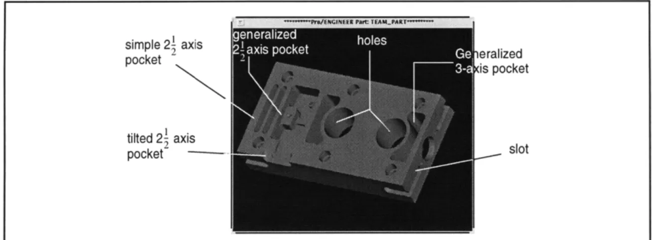
simple 21 axis pocket tilted2 axis pocket ieralized (is pocket 1 slot

next generation tools like hexapod - are not fully utilized to the fullest extent possible because of the difficulties associated with tool-path generation. In order to make machin-ing technology more accessible in today's demandmachin-ing industrial environment, it is neces-sary to explore other paradigms which may, in the future, overcome the limitations of existing approaches.

In this thesis we outline an emerging paradigm for generating multi-axis machining paths directly from the boundary representation of the geometric object. We refer to this as

Art-to-Part Machining. The key idea in Art-to-Part Machining is simple: we will

gener-ate free-form cutting paths to remove all the excess mgener-aterial from the stock while avoiding local and global interference with the embedded design. Little effort is devoted to the

organization of tool-paths into formal primitives like features. Instead, the goal will be to harness the dexterity of multi-axis machine tools using access arguments.

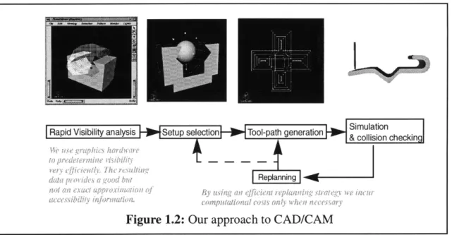
Borrowing a concept from the robotics community, tool-path generation in our strat-egy revolves around ensuring cutting tool accessibility. However, experiences in robot path planning and other fields have shown that determining exact accessibility is in gen-eral a computationally expensive process. As a practical and expedient alternative, we propose to use initial visibility analysis to approximate accessibility during the pre-pro-cessing stage. This accessibility is further refined during tool-path generation with the help of interference checking routines. These tool-paths are further validated and cor-rected during simulation and replanning stage. In this way, our approach avoids the up-front expense of accessibility analysis, only incurring it when the approximation is seen to cause interference. We show this in Figure 1.2. With this iterative strategy we hope to bring a long developing idea to practical fruition.

Rapid Visibility analysis Setup selection Tool-path generation i olsn checking

2torpI dm& collision c

Inta oIroies a good by

Replanning]-xi: , , f. n( v

Figure 1.2: Our approach to CAD/CAM

Outline: In Chapter 2 we present a brief outline of previous work in the area of CAD

and CAM. In Chapter 3, we describe how to carry out visibility analysis, and a procedure to construct discrete visibility cones. We also explain how this visibility data is used to select a minimum number of setups from which the work piece can be fully machined. A general strategy for generating tool paths is presented in Chapter 4. In Chapter 5, we return the results obtained by applying our strategy to 3-axis and 5-axis machining. We conclude the thesis by presenting the future work in Chapter 6

Chapter 2: Background

There has been a large body of work in CAD/CAM integration. Below we summarize this previous research.

Feature based machining: The concept of machining features has been an important

step in the understanding and development of manufacturing planning. Machining fea-tures have the following advantages: 1) feafea-tures are a convenient decomposition of a cad model into handleable units for high level planning; 2) tool-path generating algorithms can be developed and implemented up-front; 3) since features fit the object-oriented model well, tool selection and cutting parameter selection can be linked cleanly to knowl-edge bases; 4) machining features implicitly define access directions and accessibility vol-umes. The first mention of features is probably by Krypianou [Krypianou 80]. The concept of manufacturing features first appears in [Arbab 82]. Arbab points out the simi-larity between the boolean difference operation in constructive solid geometry and the material removal in machining. This lead to the idea of destructive solid geometry (DSG), a design input methodology later refined in a series of papers: [Hummel 86, Kramer 88, Turner 88, Cutkosky 88, Shah 88 and Gindy 89]. In DSG, the user defines a "stock" and then subtracts primitives (features) to define the part. The development of process plan-ning systems for machiplan-ning has closely followed the development of features technology. Beginning with early work by Nau [Nau 86], Hayes [Hayes 89], Anderson [Anderson 90] and Cutkosky [Cutkosky 90], to more recent papers by [Yut 95, Gupta 95, and Sarma 96], the use of features has become better understood and more widespread.

Meanwhile, there has been interesting research in feature extraction in recent years. Seminal work on feature recognition was done by Woo [Woo 82]. Later, Joshi [Joshi 88] used graph-based heuristics to extract features from adjacency graphs. [Dong 88, Sakurai

90, Finger 90 and Vandenbrande 90] made important contributions to the field. Kim extended Woo's work on convex decomposition [Kim 90]. Gadh introduced the concept of depth filters for feature recognition [Gadh 92]. Nau et al introduced the idea of generating alternative, optimal machining volumes in [Nau 92]. Recently, Regli has reported a prom-ising new approach to feature extraction in his Ph. D. Dissertation [Regli 95]. His approach is based on the extrapolation of "maximum cover features" for 3-axis machining from the faces of a boundary representation. In general, most feature-based approaches have been limited to three-axis machining.

Surface machining: The field of surface machining has been a similarly intense area of

research in the last few years. Since Faux' widely used book [Faux 81] a number of sys-tems have been developed over the years for surface machining with special emphasis on die-mold applications: [Oetjens 87, Loney 87, Kuragano 88, Chou 89]. Most early sys-tems, however, were either 3-axis based, or were relatively limited in their applicability because of problems of gouging and surface finish. Recognizing this problem, a few researchers in recent years have looked into the simulation of multi-axis cutting: [Oliver 86, Jerrard 89, Jerrard 91]. Jerrard's work was based on the Z-buffer approach. In the cur-rent work, however, we will use a voxelized model for simulation because it provides a more complete picture of the work place. We will use the Z-buffer instead for hidden sur-face removal. The issue of global interference is discussed in [Choi 89, Tseng 91 and Elber 94], and most recently by Lee et al [Lee 92, 95, 96].

Access based approaches: The problem of tool access has been approached from both,

a solids, and a surface perspective. Seminal work in the area of visibility and visibility maps was performed Chen & Woo [Chen 92, Woo 94]. They introduced the concept of visibility cones for points on a workpiece, which can be mapped on to the unit sphere to create a Spherical Map. The same authors also show how the Gaussian projection can be

extended with a central projection to manipulate access information and minimize setups. The idea of Spherical maps has been adopted by Wuerger and Gadh [Wuerger 95] to eval-uate the separability of dies. The concept of access is also handled in a feature-based approach in [Sarma 96]. The ideas of a visibility cone have influenced surface machining as well. Lee [Lee 95] uses a convex hull based approach to approximate local visibility. An innovative approach to surface accessibility is presented in [Elber 94], in which con-vex surfaces are mapped to a space in which they become planar. Obstacles to the surface are also mapped into this space, and tool-path generation is carried out in a 3D world. The paths are then inverse-mapped back to the original space to obtain 5-axis tool paths. [Spy-ridi 90, Henderson 96 & Tangelder 96] explore the concept of accessibility cones as perti-nent to 5 axis machining problem. The work presented in this paper focuses on practical and tractable methods to determine and manipulate visibility cones in a manner appropri-ate for NC tool path generation.

Commercial CAD/CAM systems: Most commercial CAM systems, including

pur-ported 5-axis systems, are based on 3 degree-of- freedom (as opposed to 3 axis) cavity

machining techniques. We use this term because, while many CAM systems like

Master-CAM, CAMAX, AlphaCAM and ProManufacture can utilize 5-axis machines, their search space is always limited to three degrees of freedom. The other two degrees of free-dom are defined by the orientation mode set by the user. Common modes are surface-nor-mal machining and drive-surface machining. In either case, the problem of path generation is reduced to a search conducted entirely on a three dimensional manifold. The problem with this limited search is that the CAM system is incapable of preventing gouges and global interference. That responsibility today lies solely with the user. Furthermore, apart from access issues, the user of commercial CAM systems must also perform

addi-tional tasks including: selecting a tool, selecting a cutting strategy, and selecting a cutting order. As a result, 5-axis machining is still very much an acquired skill today.

Recent awareness of these problems has lead to interest in a new technology called

Generative NC. SDRC has recently offered an early version of its Generative NC

pack-age. SDRC's generative NC system, however is still based on 3-axis machining, and still requires human input for access-direction selection and tool selection. This proposal deals with the theoretical and practical issues in 5-axis generative NC. There are fundamental theoretical issues that need to addressed before such a system can be created. Yet, without such research, it will be difficult to make full and efficient use of advanced 4 axis, 5-axis and multi-axis machine tools like the Hexapod.

Robot path planning: The research presented here has some parallels to previous work

in robot path planning as well. The problems of visibility and accessibility have been addressed in great detail by a number of researchers. The concept of a configuration space evolved through a series of papers in the early 80's [Udupa 77, Lozano-Perez 81, 83]. In the latter paper, Lozano-Perez also introduced the concept of cell decomposition, which is loosely analogous to the voxelized approach presented here. A comprehensive description of later developments in robot planning is presented in [Latombe 1991]. An important dif-ference between robotics and machining, however, is that while robotic path planning is concerned with accessing particular points in the configuration space, machining is con-cerned with sweeping all the points within and on the boundary of the delta-volume.

Chapter 3: Accessibility Analysis

Machining process starts by fixing the stock on a machine tool and moving the cutting tool in a predefined path. The tool removes the excess material (delta-volume) from the stock and produces the desired workpiece. The predefined path includes the curve along which the tool has to move and the orientation of the tool along the curve. In case of 3-axis machining the orientation of the tool is fixed. But in 5-axis machining the tool orientation becomes critical, as the tool has two additional angular degrees of freedom.

There are two stages in machining: 1) Roughing and 2) Finishing. During roughing the tool spans through the delta-volume removing most of the unwanted material, and during finishing the tool spans over the surface of the workpiece giving it the required finish and tolerance. To sucessfully carry out these two stages of machining, the tool orientation at various points in the delta-volume and on the surface of the workpiece has to be deter-mined.

3.1 Accessibility

An object is accessible if it can be reached. A point in free space can be accessed from infinitely many directions in R3 space. These directions are represented as points on the sphere S2. This representation can be generated by mapping the directional vector to a point on the sphere centered at the origin, where the unit vector joining the origin to the point on the sphere represents the directional vector. The set generated by mapping all the access directions of a point onto the surface of the sphere is called an accessibility map. In the present case of a point in free space, the accessibility map is the entire surface of the sphere as shown in Figure 3.1. As more obstructions are introduced around the point, the accessibility map reduces from the entire surface of the sphere to a cluster of small patches

on the surface of the sphere. The cones constructed with these patches as the base and the origin as the apex are called the accessibility cones. The earlier definition of accessibility is not concrete, as it does not quantify the entity trying to reach the object. For the purpose of machining we define accessibility as,

Accessibility: Point P on the surface of the workpiece is said to be accessible by a tool

T aligned along an orientation O, if P can be reached by T along O without violating

the following conditions,

1. Only the cutting portion of the tool is in contact with the stock material, and 2. Tool is not interfering with the embedded design

P is called the access point and O is called the access direction.

While generating tool-paths, the tool should be given an orientation along which it should be aligned at every point. In order to generate interference free tool-paths, this ori-entation should be one of the accessible directions for that point. So, to automate the

pro-cess of generating tool-paths, atleast one acpro-cess direction for every point on the workpiece has to be determined. Determining accessibility cone is of real importance in machining. However, the accessibility cone is difficult to determine.

One way to determine the access direction is by trial and error. Choose a random tool and check if it is able to reach the intended point with out any interference. Repeat the above process by changing the tool and the direction of approach till it suceeds. This approach is time consuming and unreliable. [Tangelder 96 and Roberts 96] use the Minkowski operation to generate accessibility cones. Unfortunately, Minkowski methods tend to be computationally expensive. Our approach is to find the approximate access direction, but a good estimate, very efficiently. We simplify the process by assuming the tool to be straight line. Under this assumption accessibility is analogous to visibility. We formally define visibility as,

Visibility: Point P is said to be visible along a direction O, if an ray of light from P

travelling along O reaches the outer space without interfering with the embedded design.

Visibility maps are generated by mapping all the direction along which a point is visible on to the surface of the sphere. These visibility maps are often referred to as visibility

cones. The visibility cones are processed further to determine the approximate

accessibil-ity direction. Below we discuss how visibilaccessibil-ity maps are generated for surfaces and vol-umes.

3.2 Visibility analysis

The shape of the embedded design imposes constraints on the accessibility (in our case, visibility) of various regions of the delta volume. Machining of any point in the delta volume is guided by the accessibility of that point. These constraints determine the per-missible tool size and the orientation of the tool. For error-free path planning all the

con-straints imposed by the embedded design have to be determined. These concon-straints can be determined by accessibility analysis of the workpiece. Accessibility of a point is defined for a specific tool size and orientation. A point on the workpiece is considered to be acces-sible if the delta volume around that point is machinable. It is computationally expensive to perform accessibility analysis for all possible tool sizes. Instead, we perform the analy-sis assuming the tool to be a straight line. We refer to this approximate analyanaly-sis as visibil-ity analysis.

3.2.1 Using graphics hardware

Visibility algorithms have received considerable attention in the fields of computer graphics and computational geometry. A number of algorithms have been proposed in the literature, and are summarized in [Foley 95]. However, hardware techniques, like depth buffer approach, have recently proved to be very effective. With the ability to scan convert a million polygons per second, visibility analysis can be performed very efficiently within a fraction of a second. The depth buffer is a part of video memory used for scan conver-sion. Each pixel on the screen has a memory address into which the information regarding its color and depth are written. As the polygons are scan converted, the color and depth values of the polygons that are closer to the eye overwrite the existing values, enabling hidden surface removal. This hardware approach helps in building the configuration space of the workpiece very efficiently. In essence, we propose to use 3D graphics hardware as a special purpose solid-modeling engine.

The graphics engine scan converts a model into a scene. In our case, the model is the embedded design. Graphics boards are optimized to render convex primitives. In our visi-bility analysis, we reverse this process to extract the visible part of the model from the scene. One way to do this is to do a inverse screen transformation of all the points in the

View from an array of directions.

Surfaces tesselated and color encoded for identification.

Cones of visibility for each tesselation.

Map to visibility cones This information

on the Gaussian sphere will be stored for

global interference avoidance during \

(tool

Figure 3.2: Visibility analysis

scene that are visible to get the points in the worldspace coordinates. From these points infer the part of the model that is visible. Unfortunately, this is computationally expensive. A more efficient method is to determine visibility in the object space. This strategy per-mits us to do away with the inverse transformation. This is achieved by color encoding (R,

G B) each primitive (face) in the model. The visible part of the object is extracted by

iden-tifying the colors in the graphics scene.Using the common 24 bit (R, G, B) color boards with 8 bits per color 16,777,216 different primitives can be encoded.

In standard boundary representation, faces of a solid are modeled monolithically as single entities. While convenient for solid modeling, this is not ideally suited for visibility analysis. For example, if we were to encode an entire face with one color, the occurrence of that color would not imply visibility of the entire face; it would merely imply that a tion of the face is visible. This information is not even rich enough to indicate which por-tion of the face is visible.

To perform a satisfactory visibility analysis, each face has to be subdivided into smaller entities. If all these sub-entities are visible, it may be possible to assume that the entire face is visible. Obviously, the validity of this assumption is dependent on the size of the sub-entities. In our research, instead of color encoding the faces of a BRep, we first generate a tessellated representation and then color encode each triangle separately as shown in Figure 3.2. Now, if the color assigned to a given color is visible in a certain ori-entation, we say that the entire triangle is visible from that orientation. Any errors result-ing from this assumption will be corrected durresult-ing later simulation and interference checking. Since the size of the triangles is kept small, the errors resulting from this assumption can be easily compensated.

In 24 bit (R, G, B) graphics board each color is represented as mix of R,G and B. Each color occupies 24 bits, with its components (R, G, B) occupying 8 bits each. Internally each component take a value between 0 and 255, both values included. But when the graphics buffer is queried, it returns values between 0 and 1 for each component (in the intervals of 1/255). In order to make the color encoding compatible with the internal repre-sentation of (R, G, B), the (R, G B) values for encoding are assigned as follows,

R/G/B = i/255 where 0<=i<=255

If the (R, G, B) values assigned do not comply with the above rule, then the fraction is rounded off to the nearest multiple of 1/255. This will lead to errors in identifying the vis-ible triangles, hence the visvis-ible part of the model. Note that a typical color graphics card will permit 224 triangles to be encoded in this way.

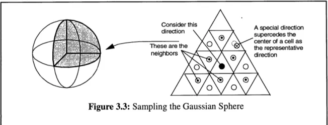
3.2.2 Sampling directions

Visibility analysis is performed along a set of pre-defined orientations. Two issues have to be considered in determining the set of orientation. Firstly, it is necessary that we

consider a fairly even sampling of the Gaussian Sphere. To achieve such a sampling, we

start with a tetrahedron and subdivide it according to Algorithm 1, till the desired

sam-pling rate is achieved. A tetrahedron is supplied as the initial input to this algorithm. At the

required resolution, the centers of the triangular cells generated in this manner represent a

fairly homogenous sampling of the sphere. The resultant triangles are called Gaussian

tri-angles to distinguish it from the tritri-angles of the model. The visibility analysis is

per-formed along the directional vector from the center of the sphere to the centroid of the

gaussian triangles generated above.

Algorithm 1: Sampling of the Gaussian Sphere

Terminology:

CreateTriangle(vl, v2, v3): constructs a triangle with the given three vertices Vertex(T, i): returns the it

h vertex of triangle T

Edge(V i): returns the ith edge connected to Vertex V of a triangle (two edges start from every vertex in a triangle)

Input:

Level of sub-division L

Set of triangles to be sub-divided T()

Output:

Set of triangles approximating a sphere To()

Algorithm:

For i= 0 To L Do

For Each T belonging to Ti() Do Forj = 0 To 3 Do v1 Vertex(T j) v2 4 MidPoint(Edge(vj, 0)) v3 MidPoint(Edge(v1, 1)) To.ADD(CreateTriangle(v1, v2, v3)) End vI MidPoint(Edge(Vertex(T, 0), 0)) v2 : MidPoint(Edge(Vertex(T, 1), 0)) v3 <- MidPoint(Edge(Vertex(T, 2), 0))

To.ADD(CreateTriangle(v_{1, v2, 3))}

For Each T belonging to T() Do

project all the three vertices of the triangle on to the surface of the sphere

END Copy TO to Ti Initialize To END END return T_O

Special directions: In addition to homogenous sampling, a second consideration

relates to the directions of innate importance to the workpiece. The adhoc sampling we have prescribed above may miss such directions. For example, consider a large plane face oriented at some odd tilt in the work piece. It is not unlikely that this face will be machined with a flat bottomed end-mill, in which the access direction will be perpendicular to the plane. This perpendicular direction may not contained in the homogenous sampling of the Gaussian Sphere. We therefore need to incorporate such special directions into the sample set as well. Some simple heuristics can be used to select and prune the special directions. For example, the perpendiculars to all flat faces in the original BRep representation must be incorporated into the sample set. It may also be necessary to incorporate linear edges in the BRep model into the sample set. It is important to exercise reason in creating the sam-ple set because too large a samsam-ple set will create computational problems later.

Neighborhood: Figure 3.3 shows how sampling directions correspond to the center of

the triangular cells created by the tessellation. Special directions can be handled as fol-lows. A special direction replaces the centroid of the triangle in which it lies as the "repre-sentative direction" for that portion of the Gaussian surface. It is possible now to define the neighbors to a particular direction as those whose cells (triangles on the gaussian sphere) contact the ones in question. There are six such neighbors, of which three cells make edge contact, and the remaining three make vertex contact.

3.2.3 Generating discrete visibility cones

To generate discrete visibility cones, visibility analysis is performed from a number of orientation arranged on the Gaussian sphere as shown Figure 3.2:. Each orientation is associated to a Gaussian triangle. For each orientation, the model is rendered and then the

(R,G,B) buffer is queried to obtain the color values of every pixel in screen space. From

the (R,G,B) values, the corresponding triangles are identified. If a triangle is visible in that orientation, then its assumed to be visible along all the directions represented by the corre-sponding Gaussian triangle.

Once the visibility analysis is completed, a set of orientations from which a triangle is visible are obtained. The set represents a region in (0, (p) space along which the triangle is visible. The cone constructed with this region as the base and the triangle as the apex, as shown in Figure 3.4, is referred to as discrete visibility cone. This information is used to determine the setup directions and tool path planning.

3.2.4 Sideways visibility

One problem with using the visibility argument is that faces parallel to the visibility direction are not usually visible from that direction. Yet, in machining, a parallel face may be accessible from a parallel direction. For example, a typical end-milling operation will

Figure 3.3: Sampling the Gaussian Sphere Consider this

direction

AThese are the

create a side face that is parallel to the direction of machining. To account for such situa-tions, we correct the visibility data generated with the side correction algorithm:

Algorithm 2: side correction Terminology:

Let v(o) be the set of triangles visible from a direction oi. Let n(o) be the set of neighboring orientations to o.

Input:

o, n(o) and v(o), the orientations and visibility data generated by direct visibility analysis. Output:

v-, the visibility data enhanced with side visibility information.

Algorithm:

For Each o' E n(o) Do d(o', o) := v(o') - v(o)

For Each t E d(o', o) Do If tl o,

Then v-L v-LIU t

Determine which triangles that have become invisible by rotating to this orientation orientations

If such a triangle is perpendicular to the given orientation Then it must be visible along the side.

3.2.5 Volume visibility

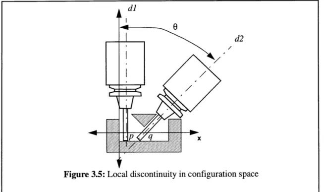
Thus far we have only considered the accessibility of points on the surface of the workpiece. To generate tool paths within the delta-volume, accessibility information of the interior is necessary. To illustrate this, consider the situation in Figure 3.5. From the visi-bility analysis we know that point p is visible along dl , and point q is visible along d2. But, there is no information available about the admissible tool orientations along pq . One way to generate this information is to interpolate between dl and d2 .This might be satisfactory for most of the cases, but there exist some cases where this might lead to tool-workpiece interference as in Figure 3.5. To prevent in the interior interference, accessibil-ity information for the entire delta-volume has to be generated. We call this volume

visibil-ity.

The delta-volume is a continuous 3-dimensional region. It is necessary to digitize or sample this space in order to map visibility. We use a simple three dimensional space enu-meration of the delta-volume, also referred to as a voxelized representation. We convert B-Rep to voxels by a simple scan-conversion algorithm [Foley 90, Samet 91].

d2

q/

We compute volume visibility by extending the surface visibility information obtained earlier. From the visibility analysis, each point on the surface of the workpiece has a set of orientations along which it is visible. Now, we cast rays from the point along each of these orientations, and tag all the voxels touched by these rays. By taking the advantage of coherence along a line, volume visibility can be computed in this way with minimal com-putational effort. Algorithm 3 summarizes the approach. The data generated by voxel visi-bility is five dimensional (x, y, z, 0, () . To store this data in a ordinary data structure is expensive. A hierarchical data structure like a 5-d tree can be used. Currently, memory limitations demand that we use only a coarse voxel grid. However, we are developing hierarchical data-structures in on-going research. The volume visibility cones look similar to the discrete visibility cones shown in Figure 3.4.

Algorithm 3: Volume visibility

Input:

Orientation O(0, p) Triangular mesh T

Visible triangles (from visibility analysis) VT number of triangles visible triangleNo Voxel array data structure VOX[x, y, z, 0, 0]

Output:

Filled voxel array data structure VOX[x, y, z, 0, #]

Terminology:

tag_voxel(): appends the visible orientation to the voxel Algorithm: Cx - cos(0) sin(p) Cy - sin()sin(p) Cz - cos(p) vertexNo <- 3 For i <- 1 To triangleNo Do For j <- 1 To vertexNo Do

X - get_xcoord_vertex(T, i,j) Y < get_ycoord_vertex( T, i, j)

Z -- get_zcoord_vertex(T, i, j)

While Xmn < X Xmax and Ymin Y Ymax and Zm < Z < Zmax Do tag_voxel(VOX[x, y, z, 0, 0])

X - X + Cx Y<- Y+ Cy

Z -- Z+ Cz return VOX

3.2.6 On the resolution of the graphics approach

Although the use of graphics hardware is not central to our approach, we have pre-sented it here as a means to accelerate the visibility analysis. A potential problem with the graphics approach is loss of resolution in the use of tessellations and pixels. Fortunately, experiments show that inaccuracies in our approach are insignificant, and the graphics approach is indeed viable as we elaborate below.

Typically, each triangle we create is about 50 pixels in area. We scale the part to ensure that this is the case. Given that there are a limited number of pixels on the screen, this does constrain the resolution of the tessellations we can handle. However, for faces in the size range of 50 mm, this means that triangles can be as small as 1 mm on the side. At a 50

ori-entation, the same triangle occupies a projected area of only 5-10 pixels. Assuming that the triangle started out as an equilateral triangle (it is important to start with a reasonably well formed triangulation), the minimum width of a triangle oriented at 50 to the viewing direction is at least half a pixel. Therefore, at a 50 orientation, it is very unlikely that we

will lose a triangle in the graphics based visibility approach. Our experiments have con-firmed this to be the case; thus far losses due to granularity have been insignificant. When losses do occur, it is relatively inexpensive to correct them using algorithms like the side-visibility algorithm described earlier. The surface error caused by a triangulation of lmm

is within 10-6 mm and 10-3 mm respectively in the typical prismatic and curved compo-nents we have sampled.

Another potential source of granularity is the fact that we use a discrete set viewing directions. For example, a cylindrical hole is completely visible only along the axis of the cylinder. A problem might occur if this axis does not coincide with the viewing directions selected as a sample set; the resulting tool paths will obviously be very inefficient.

We combat this problem by including special access directions in addition to the sam-ple set generated around the Gaussian Sphere. These special access directions include, for example, the perpendiculars to large flat faces and the axes of cylindrical holes. This ensures that the sample set does not exclude an obvious access direction, and thus incur huge inefficiencies.

3.3 Setups

The tool path is a 3D curve that defines the motion of the cutting tool. Before starting any machining operation, it is necessary to immobilize the workpiece in a certain orienta-tion. These orientations are called the setups. In the interests of efficiency, it is necessary to minimize the setups during work holding. Note that we will not discuss fixture planning in this paper. We will assume that the workpiece can be fixtured in any setup [Sarma 96].

The issues involved in determining the setup directions in 3-axis machining are quite different from those in 5-axis machining. One definition of the setup minimization prob-lem is as follows:

Determine the minimum number of orientations oi such that

the set of triangles ya(oi)

is the set of all triangles on the surface of the workpiece. In other words, find the min-imum set of orientations from which the component is completely accessible. In our anal-ysis, we approximate accessibility with visibility.

The visibility data is available to us from the visibility analysis conducted over a large number of sampling directions. Finding the minimum number of setups reduces to the

minimum cover problem. The general version of this problem is NP-Complete [Garey 79].

One approach to the set cover problem is the well known Quine-McCluskey Algorithm, which has been used extensively in the field of logic synthesis.

3.3.1 The Quine-McCluskey Algorithm

The Quine McCluskey algorithm can be applied directly to our application as follows.

If m is the number of sampling orientations and n the number of triangles, we create an m

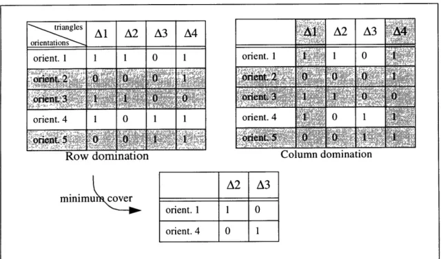
x n matrix in which the rows correspond to orientations and the columns to triangles. If a triangle is visible from a certain orientation, we mark that element as 1. If not the element is 0. We refer to this as the visibility matrix, and show it in Figure 3.6:.

minimu cover 0 0

Al

4

The Quine-McCluskey Algorithm proceeds by a series of alternating row and column dominations.

Row dominations: A row j dominates a row i if every triangle visible from orientation i is also visible from orientation j. In this case, we delete row i. Row dominations cor-respond to the elimination of unfavorable orientations.

Column dominations: A column p dominates a column q if triangle q is visible from

every direction in which triangle p is visible. When column p column-dominates col-umn q, we eliminate colcol-umn q. Colcol-umn dominations correspond to the identification of hard-to-see triangles, which are more critical in defining the final setups.

The Quine-McCluskey Algorithm proceeds by reducing the size of the visibility matrix with alternating searches for row and column dominations. After at most o(n3) steps, the algorithm may stall, as no row or column dominations may be available. The visibility matrix at this point is referred to as the cyclic core. In this situation, it becomes necessary to start checking if combinations of rows or columns dominate other rows or columns. This is essentially a brute-force search, as would be expected at some point in an NP-Complete problem. However, the initial application of the Quine-McCluskey algo-rithm usually reduces the search space enough to make the brute-force technique viable.

Note that if all the elements in a column are 0, then the part is unmachinable, because that triangle can not be accessed. On the other hand, if all the elements of a certain row are zero, then that orientation can be deleted without further consideration, as it is ineffectual. The result of the Quine-McCluskey Algorithm applied in this manner is a minimum set of directions from which the entire surface of the workpiece is visible.

3.3.2 Biasing for parallel and perpendicular directions

Unfortunately, the orientations obtained by this technique may be optimal interms of the number of setups, but not necessarily optimal for machining. This is because in machining it is preferable, as far as possible, to orient the tool perpendicular or parallel to

the surface. This is especially important in 3-axis machining where the setup directions determine the orientation of the tool, and the resulting digitizing effect. The algorithm pre-sented in the review section therefore needs to be biased towards orthogonal setups. We state this as follows:

Observation 2: It is preferable to access a face from a perpendicular or parallel direc-tion [Chen 92].

We refer to this as the parallel-perpendicular (PP) heuristic. To incorporate PP heuristic we use a multi-valued version of the Quine-McCluskey Algorithm. The elements of the visi-bility matrix will be assigned a number as follows:.

element [ij] = 2 when:

the angle between orientations i and triangle j is greater than 800

or less than 100,

and triangle j is part of a flat face f

and every other triangle in f is visible from orientation

•1

= 1 when the angle is between 10 0 and 80 o and triangle j is visible

from direction i

= 0 when triangle j is not visible from direction i

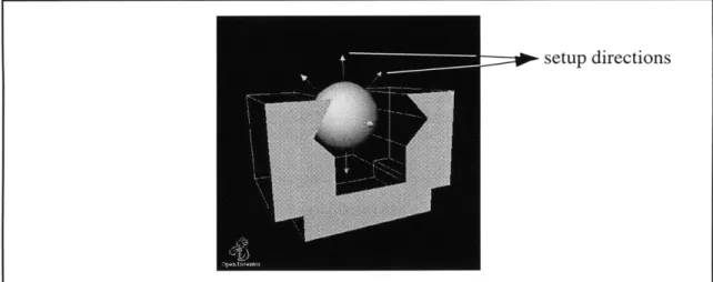
In other words, we assign a higher weight to flat faces that are entirely visible from a cer-tain direction. We then use the following ordering to determine dominance: 0 < 1 < 2. A row i dominates a row j if every element of i dominates the corresponding element of j. Column domination can be defined similarly. This approach biases the Quine-McCluskey Algorithm towards "orthogonal setups" by blocking the domination of important PP ori-entations. An example of the output of this analysis is shown in Figure 3.7:.

1. Notice that edge conditions like fillets and sharp corners can also be considered in the analysis at this point. For example, there is no point approaching a face from a parallel direction if the edge-conditions of the face are all sharp corners. Parallel access leaves fillets.

! setup directions

Setup direction obtained by performing the visibility analysis from different directions arranged on the

Gaussian sphere, and biassing the Quine-McCluskey algorithm towards the PP directions. Figure 3.7: Setup directions

The performance of these algorithms thus far has been very promising. Typically, the size of the cyclic core is in the order of 10-20 orientations. At this point, enumerative anal-ysis becomes viable and inexpensive. Typical situations involving 5,000-10,000 triangles, and 300-1,000 sampling orientations, can be handled within a few minutes of user time on a standard workstation.

3.3.3 Conclusion

Generating accessibility information is very important in machining. Unfortunately there is no easy and straight forward way of dealing with it. Most of the known methods, like Minkowski operation, are computationally expensive.

We simplify the process by assuming the tool to be a straight line. Under this assump-tion accessibility is analogous to visibility. We perform visibility analysis from a set of ori-entations arranged on the Gaussian sphere. Discrete visibility cones are constructed for each triangle in the model by keeping track of the orientations along which that triangle is visible. These visibility cones are used in the setup selection and in determining the

approximate accessibility direction. Determining the approximate accessibility direction is discussed in the next chapter.

Chapter 4: Tool path generation strategy

Our aim is to machine the delta-volume and produce a work piece of specified finish and tolerance. This is achieved by generating tool paths to machine the delta-volume. Tool path has two components: the path along which the tool must move and the orientation of the tool along the path.

In the previous chapter we discussed the process of generating discrete visibility cones for a triangle of the model. These cones represent the region through which a ray of light can reach the triangle with out interfering with the embedded design. But, since the tool is of a fixed diameter, all these orientations cannot be legal. In this chapter, we will illustrate the process of determining the approximate tool orientation from the discrete accessibility cones.

There are many techniques discussed in literature to generate tool paths. None of these techniques are capable of generating tool paths automatically for a complicated part. Our approach, discussed below, is more general and helps in automated tool path generation.

In our approach we remove the delta-volume in two stages. In the first stage, the bulk of the volume is removed using a heavier tool. We refer this stage as gobal roughing. In the second stage, faces of the workpiece are considered one at a time and then a tool is used to remove material at a finer rate to leave the workpiece surface with the required fin-ish and tolerance. We refer to this stage as face-based finfin-ishing.

4.1 Global roughing

Roughing is a rapid material removal process, generally involving heavier but less

Global

feature

(a)

Feature based description is awkward.

Features must be extracted and tool-paths

generated individually for each feature. Resulting paths likely to be redundant. Inappropriate tools may be selected based on features (instead of largest tool).

(b)

Global roughing: Tool-path is generated directly from geometry. Maximal tool is selected, and there are no redundant cuts,

Multi-axis tool path "searches" for delta-volume

Figure 4.1: Global roughing: A simple example

material before finishing operations. In the previous chapter, we described some general visibility techniques to aid global interference avoidance. In this section we show how roughing can be performed regardless of the individual features. The basic idea of Global

roughing is illustrate Figure 4.1.

At this stage, we assume that the fixturing and the setup details are taken care of. Fix-turing has to be taken care by the user. Setup selection can be done by the modules described in the previous chapter or can be user defined.

4.1.1 Slicing the tessellated model

The program receives the part in a pre-determined posture. The tessellated representa-tion is sliced at a sequence of depths perpendicular to the setup direcrepresenta-tion. The slice plane intersects some of the triangles of the model. We extract the line along which the triangles intersect the slice plane. These lines are grouped together, based upon the neighborhood information of the triangles in the model, to form closed contours. This process could gen-erate more than one closed contour. Some of the contours correspond to the embedded design and some of them to the delta volume. In addition to the above contours we also generate a contour corresponding to the stock. Figure 4.2-a shows the contours generated

by slicing the embedded design. Machinable contours are generated by identifying the contours corresponding to the design that are contained within a contour corresponding to the delta volume, as shown in Figure 4.2-b.

4.1.2 Contour Offset

We generate centerline tool paths to remove the delta volume. The center of the tool follows this path during the process of machining. These tool paths cannot proceed all the way to the boundary of the contour, as the tool would gouge into the embedded design. To prevent this, the contour has to be offseted non-linearly by distance d given by,

d = D/2cos(O)

0 is given by the angle the tool makes with the setup direction

As mentioned earlier, the contour is constructed by grouping together the line seg-ments obtained by slicing the tessellated model. So, each line has a corresponding triangle in the tessellated model. In the previous chapter, we constructed discrete accessibility cone for each triangle. The angle at which the tool should be oriented with respect to the setup direction, when it is in the neighborhood of a particular line, is obtained by processing the accessibility cone of the corresponding triangle. The procedure to do this is illustrated later in this chapter.

Pseudo codel: Non-linear offset

Given:

Machinable contour (One outer contour and zero/more islands) Normal direction N of the outer contour

Tool diameter D

stepl: Number the elements (line segments) of the outer contour in the counter clockwise direction and

the elements of the islands in the clockwise direction. Arrange the vertices of the contour elements such that their directional vector points in the direction as shown in the figure below..

i 8

4

5, 7 9

6 10

Stepl

step2: For each element i in the contour, find the orientation(explained in the next section) the tool has

to approach in order to machine the material in its neighborhood. Find Theta which is the angle between the tool orientation and the setup direction

step3: Offset the element i by a distance D/2cos(O) in the direction given by N X Di, where Di is the directional vector of element i and X represents the crossproduct between two vectors..

step4: Consider two successive elements i andj in that order. If the angle between them is less than 1800

then eliminate the part of i that is between the point of intersection and the end of the line, and part of j that is between the start of the line and the point of intersection. If the angle in greater that 1800, then there will be a gap between the two offset lines. Connect these two lines with a part of a ellipse. The equation of the ellipse is got by solving the equation of a conic section with CO continuity (end point of the first line and the start point of the second line) and Cl continuity (slopes of the lines) as the

bound-ary conditions. At this stage, the offset elements of an individual contours when put together form a

angle more than 1800 lines are connected by

an ellipse

angle less than 1800 lines are pruned.

step4

closed contour called the offset contour. But if the offset distance is too large then the offset contour might have self intersecting loops. Loop elimination techniques have to be used to eliminate these

loops.

step5: Once step4 is performed for the outer contour and the islands, perform an union of all the offset

contours corresponding to the islands.

step6: Subtract the resultant contour of all the islands from the offset of the outer contour.

step6

The offset contours obtained from this step are then associated with the voxels that they occupy. These voxels are used to harness the voxel visibility data derived during the visibility analysis. There are three levels in this analysis, at increasing levels of scale. We describe them in order in this section. The first stage is concerned with orienting the tool, in a single voxel, and we describe it in Section 4.1.3 below. The second stage is concerned with interpolating a tool path between two adjacent voxels, and we describe it in Section

4.1.4. Finally, at the most global scale, we are interested in stringing together a tool path that covers the entire slab. We describe this in Section 4.1.5.

4.1.3 Orienting the tool in each voxel

Our approach is to tackle the tool path problem at the most local level and to build a global path from local information. In this section we describe how to orient a tool in a particular area of a slice, namely, the region inside one voxel. We are not concerned with moving the tool sideways from voxel to voxel in this section. We address that problem in 4.1.4, entitled "Voxel-to-voxel transition"

4.1.3.1 Access direction from visibility cones: cone thinning in voxel roughing

In the previous section we described how it is possible to generate visibility cones rap-idly from a tessellated approximation of an object. In reality, however, visibility does not imply accessibility. Whether a point on the workpiece is truly accessible depends on the shape of the tool, which we have not determined yet. The question we ask is which is the most effective direction from the point of view of access? We ignore questions of admissi-bility in this discussion, as it is not pertinent to roughing.

Thinning: We argue that in the absence of any information about the cutting tool, the

best access direction is in some sense the "center" of the visibility cone. The are several measures of the center. One would be to find the "center of mass" of the cones. However, this would not work because the center of mass of a complex shape might lie outside the boundary of the shape. A more appropriate "best direction" is the skeleton of the visibility patch on the Gaussian sphere. As shown in Figure 4.3, the skeleton may be obtained by thinning the tessellated representation of the visibility cone on the Gaussian Sphere. The thinning we have shown is similar to that used in computer vision applications with two important differences: firstly, we are using triangular rather than square cells, and

sec-Stage 1 of thinning

A "central" access direction S age 2 of thinning

Skeleton

Visibility cone , V V

Figure 4.3: Cone thinning

ondly, the thinning is being carried out on the surface of a sphere. The algorithm consists of an iterative thinning step with a stopping condition. The iterative step consists of start-ing from the original visibility cone, and shrinkstart-ing the outer boundary inwards one layer at a time. We define a layer as all the triangles that contact the boundary. After each shrink-ing step, as shown in Figure 4.3, we move the boundary inwards and repeat the process iteratively. We stop the iteration when the next step will reduce the shrinking region to an empty step. In practice, we can achieve this by continuing the iteration until the shrinking region goes to an empty set, and then backing up one step. The entity that remains at this

stage is the skeleton.

Accounting for machine limits; restricted thinning: Machines have motion limits. In

any setup, there are limits on the orientations that a 5-axis machine can achieve. For exam-ple, most 5-axis machines with trunion tables have a 1100 limit on a axis rotation. Similar, most rotating heads have a limit of about 700 of b rotation. These limits must be consid-ered during machining. We do so in the cone thinning stage as shown in Figure 4.4 using a process known as restricted thinning. Restricted thinning is performed on a primary

con-Stage 1 of thinning

Figure 4.4: Accounting for machine limits

tour, but restricted to a secondary contour. The steps in restricted thinning are identical to those described in the section above. However, the stopping condition is different. Instead of stopping just before the shrinking region vanishes, we stop just before the intersection of the shrinking region with the secondary contour region vanishes.

4.1.3.2 Profiling: Selecting tools and tweaking orientations

Once a reasonable access direction has been determined as described above, our next step is to pick an appropriate size of tool and to "tweak" the access direction to ensure that no collision takes place. We do this with a geometric test that we refer to as profiling. The purpose of profiling is to ascertain what the possible collisions are if a tool is placed in the orientation suggested by access analysis as discussed in the previous section. We compute the local profile with a test cylinder consisting of a tessellated surface with embedded tes-sellated discs as shown in Figure4.5 (a). Since we are interested primarily in local interac-tion, the profile cylinder should be of a diameter only slightly larger than the largest tool that we are likely to use in roughing. In this sense, profiling can be thought of as a way to determine the shape of the part in the local proximity of the particular tool posture.

Motion limits of a axis

Restricted visibility cone, due to machine limits

When the test cylinder is intersected with the workpiece in the given posture, we obtain a collision profile as shown in Figure 4.5 (b). Typically there should be no colli-sions because the access direction has already been picked with this consideration in mind. In such cases we can use the largest tool available for that point of the delta volume. How-ever, at the extremities of the delta volume, collisions are not unlikely. When they do occur, there are two ways to address to the problem, listed in order of priority are as fol-lows. The first option is to tilt the tool to avoid collisions. After this, the only option may be to assign a smaller tool. It is also possible that a voxel cannot be accessed in this setup by one of the tools available. Algorithms for evaluating these options are given below.

Pseudo code2: Tool-Profiling

Given:

A triangulated tool model(TM) divided into even number of zones in the circumferential direction A triangulated object model(OM)

preliminary estimate of the tool orientation and machining position

Pseudo code