Atmospheric propagation effects on radio interferometry

Atmospheric Propagation Effects

on

Radio Interferometry

James Louis Davis B.S., Michigan State University

(1981)

Submitted in Partial Fulfillment of the Requirements for the

Degree of

Doctor of Philosophy at the

Massachusetts Institute of Technology April, 1986

© Massachusetts Institute of Technology 1986

Signature of Author: JW I n

Department of Earth, Atmospheric, and Planetary Sciences

7 April, 1986

Certified by:

Irwin I. Shapiro, Thesis Supervisor

Accepted by:

Chairman, Department Committee on Graduate Studies

T'iC

Atmospheric Propagation Effects

on Radio Interferometry

by

James Louis Davis

Submitted to the Department of Earth, Planetary, and Atmospheric Sciences of

the Massachusetts Institute of Technology on April 7, 1986 in partial fulfillment of the requirements for the degree of Doctor of Philosophy in Geophysics.

Abstract

The technique of very-long-baseline interferometry (VLBI) offers geodesy the

potential of estimating distances on the earth of several thousand kilometers with

uncertainties of a few centimeters or less. Since the completion of the Mark III VLBI system-which combines group-delay measurements at two widely separated frequency

bands to estimate ionospheric refraction-the source of error that limits this accuracy has been thought to be refraction by the neutral atmosphere.

The largest component of the radio refractive index of air is due to the dry atmosphere. The integrated effect of this component can be estimated quite accurately from the surface pressure for a signal arriving at the site from the zenith direction. For a signal arriving from other directions, a model for the atmosphere must be combined with surface meteorological measurements to estimate the propagation delay. The

accuracy of this estimation is limited by the accuracy of the atmospheric model. The remaining component of the radio refractive index of air is due to water vapor. Water vapor in the lower troposphere is unmixed, and its effect on the group delay can vary from 0-20% of the effect of the dry atmosphere. The wet delay" is very difficult to model using measurements of surface meteorological parameters.

In this thesis, we attempt to develop an improved model for the elevation-angle dependence of the diy propagation delay. We first show that systematic, elevation-angle dependent errors in estimates of baseline length using the Marini mapping func-tion are of order 5 cm for 8000-km baselines. We hypothesize, based on analysis of the

are caused by errors in the Marini mapping function. We derive an improved

map-ping function from the analysis of ray-trace studies utilizing a parametrized model atmosphere. The propagation delay predicted by this new mapping function differs

from ray-trace results by less than 5 mm at all elevation angles above 50 elevation. We

present the initial testing of this mapping function using VLBI data, and show that es-timates of baseline length, which had shown systematic behavior, show no perceptible systematic behavior with the use of the new mapping function.

In order to test further this new mapping function, we undertook a series of

special VLBI experiments. These experiments include a large number of observations from low elevation angles. Thus far, we have analyzed eight of these "low-elevation"

experiments, and we present their results. The estimates of the Mojave-Haystack baseline length from these experiments possess a weighted-root-mean square

repeata-bility of -4 mm when the data are analyzed using the new mapping function, whereas the repeatability is 10 mm if analyzed using the Marini mapping function.

Fur-thermore, these latter estimates show evidence of temperature-dependence. These tests are consistent with-but not conclusive proof for-the conclusion that the new mapping function has adequately modeled the seasonal behavior of the propagation

delay.

We also discuss the technique of water-vapor radiometry. The derivation of the

dual-frequency algorithm employing opacities as the "observables" appears for the first

time. We point out several important features of this algorithm, and discuss possible

sources of error. We also compare estimates of the wet propagation delay obtained

from WVR data located at the Mojave site during the low-elevation experiments and processed with the dual-frequency algorithm to estimates of that delay obtained from VLBI data processed with a Kalman filter. The short term behavior of these two series

of estimates is shown to agree quite well at the level of less than 1 cm, but there are biases between the two series with apparently seasonal behavior with an amplitude of nearly 2 cm. We hypothesize that this seasonal behavior can be attributed to the use of a constant value for the dual-frequency weighting function; recent studies have

indicated that this value has a seasonal variation.

Thesis Supervisor: Dr. Irwin I. Shapiro

Paine Professor of Practical Astronomy, Harvard University Professor of Physics, Harvard University

Acknowledgements

The completion of this thesis would not have been possible without the support

of many people. I would at the outset like to thank my advisor, Irwin Shapiro, who by guidance and example has taught me something of the method of scientific inquiry, for which I will always be grateful.

A special thanks - x +to Tom Herring, who through daily discussions has

contributed immensely to this th and to my education; he has spent a great deal

of his time guiding me through the intricacies of data analysis.

I would like to thank Brian Corey and George Resch for their time spent with me

discussing water-vapor radiometers and the fundamentals of radiometry. Brian Corey

also provided commentary and suggestions for the improvement of Chapter 2, and I

am especially grateful for his continuing interest in water-vapor radiometers despite

many frustrating experiences.

A source of information and enthusiasm has been Gunnar Elgered. I would especially like to thank him and his wife Vanda for their hospitality. I would also

like to acknowledge the contributions of the entire WVR group at Onsala, Sweden, supervised by Bernt Ronnang. These important contributions can be seen at various points throughout this thesis.

The "low-elevation" experiments would not have been possible without the help from the people at Interferometrics, Inc., including Nancy Vandenberg, Dave Sche'rer,

and Steve Janoskie. I would also like to acknowledge Mark Hayes, Ed Himwich, and

Goran Lundqvist for their contributions to the study of water-vapor radiometers.

Others to whom I would like to express my gratitude for a number of diverse reasons include John Ball, Tom Clark, Ioannis Ifadis, Mike Janssen, Jan Johansson,

Chopo Ma, Jim Moran, Doug Robertson, Alan Rogers, Shoshana Rosenthal, Jim Ryan, Jeanne Sauber, John Webber, Alan Whitney, and Al Wu.

Several people from my past" deserve my thanks for having an especially great influence. They include Donald Collins, Bill Harlow, and Jerry Nolen. I would also

like to express my gratitude to my parents for their encouragement and guidance.

Finally, I would like to dedicate this thesis to Julie Kovacs: friend, fellow graduate

student, scientist, and wife.

This work was supported by the National Aeronautics and Space Administra-tion, grants NAG5-538, NAS5-27571 and NGT-22-009-904, the National Science

Foundation, grants EAR83-06380 and EAR79-20253, and the Air Force Geophysics

Table of Contents

Introduction.

1 The Atmospheric propagation delay

...

1.1 The effect of propagation media on the group delay

1.1.i The equation for the atmospheric propagatior

1.1.ii A note on units and terminology ..

. .

1.2 The refraction of radio waves in the atmosphere

1.2.i The ray-trace equations ... 1.2.ii The refractivity of air ... 1.2.iii The dry atmosphere.

1.2.iv The refractivity of moist air . . . 1.2.v Dispersion in the atmosphere ...

1.3 Modeling the atmospheric delay: some definitions

1..i The zenith delay.

1.S.ii The mapping function . .

1.8.iii The wet and dry delays . . . . . . . .

1.4 Treatment of the atmosphere in VLBI data analysis.

1.4.i Parameter estimation from VLBI data 1.4.ii Modeling the propagation delay

1.5 Effects of atmospheric modeling errors .

1.5.i Mapping function errors . . .

1.5.ii Azimuthal asymmetry ... 1.5.iii Zenith delay errors ...

1.5.iv Summary . . . . . . .

1.6 Treatment of the atmosphere in VLBI data analysis.

. . . 9

...

13

1.6.i Treatment of the time-variability of the atmosphere: Reweighting 81

1.6.ii

Estimation

of

atmospheric

parameters

. . . .... 85

2 Water-vapor radiometry ...

...

87

2.1 Relating the wet path delay to radiometric quantities ... 88

2.2 Absorption of microwaves by t:

2.2. i The 22.255 GHz line o

2.2.ii Oxygen ...

f water vapc

. . . I

2.2.iii Liquid water.

2.3 The dual-frequency algorithm .

2.4 Instrumental effects.

2.4.i Instrumental precision .

2.4.ii Instrumental accuracy

2.5 Calibration of the WVR.

2.5.i Instrumental precision

2.5.ii Instrumental accuracy

2.6 Accuracy of the dual-frequency algorithm

2.6.i Error in Tbg 2.6. ii Error in T ff.

2.6.iii Error in o

....

2.6.iv Error in W ...

2.7 Alternative dual-frequency algorithms

2.7.i Linearized brightness temperatures 2.7.ii The profile algorithm

2.8 Multichannel water-vapor radiometers

2.8.i Elimination of r0 2

2.8. ii Three close frequencies

3 Development of a new mapping function for the

3.1 Evidence for mapping function errors . . . 3.2 Ray-tracing ...

3.3 Defining the mapping function . . .

"dry" atmosphere

4 Experimental results ...

4.1 "Low-elevation" experiments ....

4.1.i

Sites

...

. .

4.1.ii Radio Sources ...

...

91

4.1.iii Observing schedule . 4.1.iv Data processing.

4.1.v Standard solutions"

...

4.2 Accuracy of the dual-frequency WVR algorithm .

4.2.i Short-term accuracy ...

4.2.ii Seasonal variations ...

.

4.3 Testing the mapping function.

4.S.i Elevation-angle cutoff tests. 4.S.ii Seasonal variations

4.4 Treatment of the atmosphere in VLBI data analysis.

4.4i The Kalman filter.

4.4.ii Estimating atmospheric

parameters

. . . . . . . . . . . . . . . . . . . . . . . . . . . . .* . . . . . . . . III . * . . . . . . . .

Conclusions

...

Appendix A: The CfA-2.2 mapping function.

Appendix B: The small scale horizontal distribution

of atmospheric water vapor . . . .

B.1 Stochastic processes and linear time-invariant systems

B.2 Statistical description of atmospheric turbulence

B.3 The model .. . . . .. . .. . . .

B.4 The observations . . . . B.5 Analysis of the observations . . . .

B.6 Modeling the input: an example . . . . .

B.7 Comparison with other observations and conclusion

References . . . . 184 188 191 197 198 208 212 212 218 225 226 228 231 . . . .. . .234 250 250 254 257 259 266 272 274 278 . . . . . . . . .

Introduction

The phenomena of absorption, scattering, and refraction are all macroscopic and familiar effects of the terrestrial atmosphere on visible light. Th blueness of the sky, the redness of the setting sun, the haziness of the moon, and the blurriness of images above a hot road are everyday spectacles. The atmosphere affects the propagation of electromagnetic radiation at all frequencies, of course. In analyzing data obtained from radio interferometric observations, the effects of the atmosphere at radio wave-lengths are most obviously of prime importance. In order to use these data to estimate parameters of geodetic, geophysical, or astronomical importance, the effects of the at-mosphere must be understood and incorporated into the theoretical models that relate

the data to the parameters of interest. If one cannot obtain some outside" estimate of the atmospheric effects, then theoretical expressions for the effects must be

devel-oped and parametrized in terms of quantities that can be estimated along with the interesting parameters.

For the analyst of modern very-long-baseline interferometry (VLBI) data com-posed of group or phase delays, and phase-delay rates, the most significant atmospheric

effect is the refraction of radio waves. Atmospheric absorption and :cattering will at-tenuate the original radio signal, which will decrease the precision of the observable, but atmospheric refraction induces an effective delay which, as mentioned above, must

be measured independently or modeled with parameters estimated using the VLBI data. The total effect is quite large: the delay induced by the atmosphere for a radio

arriving in directions of lower elevation angles, the effect increases, and is about 10 m at 10° elevation, for example.

The simplest way to deal with the atmospheric delay would be to leave it out

of the theoretical models; however, previous researchers have come to the conclusion

that the resulting errors in estimated parameters of importance are intolerable. Much

effort has therefore been spent to develop mathematical models for this delay. These efforts have been aided by the fact that the atmosphere of the earth is very well

behaved in terms of its vertical structure, being very nearly in a condition of hydrostatic equilibrium, and having a constant mean molecular weight up to about 80 km, due to vertical mixing. These facts allow the prediction of the electrical path in the vertical

direction, and hence the propagation delay in that direction, based solely on the surface

pressure, regardless of actual temperature structure. (The propagation delay in this

direction is know as the zenith delay".) Complications arise, however, when one

tries to predict the propagation delay for radiation arriving from other directions; the propagation delay then does depend on the temperature structure. Furthermore, the presence of water vapor, the local density of which can vary greatly both spatially and

temporally, can contribute significantly to the propagation delay in all directions; this

variability makes this contribution all but totally unpredictable using only theoretical

models based on local meteorological conditions at the receiving location.

From the beginning of VLBI, it was realized that in order to take full advantage

of the data obtained by this technique, the effect of tropospheric water vapor on

the propagation delay would have to be overcome. (The problem of predicting the

solved by existing models designed primarily for use in satellite tracking.) A promising

instrument known as a water-vapor radiometer (WVR) was studied by several groups, and their results indicated that the WVRy could be used to estimate the contribution of water vapor to the propagation delay (the "wet delay") with an accuracy of about

5 mm. These WVR's basically used the same design developed by Dicke in the 1940's to measure the strength of the 22 GHz line of water vapor, except that a second frequency was used to subtract the effects of liquid water (and, of course, the WVR's possessed updated electronics).

In the early 1980's, several VLBI sites as well as mobile VLBI systems started to

become equipped with WVR's. In the United States, these WVR's were built at the Jet Propulsion Laboratory under the direction of George Resch. Two of these WVR's

were mounted on mobile VLBI systems, while the fixed stations at Haystack/Westford,

.,v ens Valley, Ft. Davis, and Mojave each received one. An independent effort by

Gunnar Elgered and Bernt R6nnang also provided the Onsala Space Observatory in Sweden with a WVR.

The next step was to prove the necessity and the sufficiency of the WVR as a calibration tool in VLBI data analysis. Although it seems that in light of the previous discussion concerning the variability of water vapor the necessity of the WVR might seem to be an obvious premise, rather than something which needs proving, up to

that time there had not been any direct evidence in the VLBI data of the effects of

water vapor. Thus, the actual size of the errors in the geodetic parameters induced

by errors in the wet delay were unknown. Furthermore, it was not known whether

of inversions relating atmospheric brightness temperature to wet path delay is the

"best." Of course, if the existing WVR's were able to prove their own necessity, then that would go a long way towards proving their sufficiency.

The strategies for testing the WVR were at that time limited in number. Basi-cally, they all were based on the idea of "trying out the WVR data on the VLBI data

to see if anything gets better." The anything" could be the RMS residual delay, or

the repeatability of independent estimates of a particular baseline length or station

position, or anything else that might be affected by errors in calibrai.ng the wet delay.

The first hurdle to be overcome was obtaining WVR data simultaneously with a

VLBI observing session. The WVR's at the U.S. sites all experienced severe mechanical difficulties such that they were inoperable for a large fraction of the time. Furthermore,

the early data taken with these WVR's were extremely noisy, which was later shown to be due to imprecise determinations of the instrumental gains. As a result of these

problems, no real conclusions could be reached as to the necessity for, or the sufficiency of, the WVR.

One of the primary subjects of this thesis is the subsequent research devoted to

obtaining precise estimates of the wet delay from these WVR's, and employing these

estimates to evaluate the concept of water-vapor radiometry. This research is discussed

in Chapter 2. Chapter 1 reviews the effects of the atmosphere in VLBI, discusses propagation in the atmosphere, and describes how models may be developed for the predictions of these effects. In Chapter 3 and Appendix A, we discuss the development of a new model for the elevation-mapping of the dry part of the atmosphere, which, as will be described, was necessitated by the research on WVR's. In Chapter 4, we present

the results from a series of VLBI experiments intended to study the elevation-angle behavior of the propagation delay and our ability to model this delay.

It should be noted that as this thesis is being written, there is much happening in the area of WVR's. The WVR's originally built by JPL have been rebuilt and are

reappearing as instruments like the originals, but more precise and hopefully more durable. Furthermore, a different design is being implemented for a new series of WVR's. The discussions in Chapter 2 of accuracy and precision of WVR's will not

apply to the WVR's with this newer design, and because these radiometers have three

frequency channels, the discussions in Chapter 4 of the accuracy of the dual-frequency algorithm may also not apply.

Chapter 1

The Atmospheric Propagation Delay

Introduction

In this chapter, we will discuss the manner in which the atmosphere affects the VLBI data, and how this effect may be taken into account in the model. We will begin in Section 1.i by writing down in its most general form the equation for propagation delay due to the atmosphere. In Section 1.2, we will discuss several specific properties

of the refraction of radio waves in the atmosphere, including determination of the rav-path, refraction in a spherically symmetric atmosphere, the structure of the refractivity in the atmosphere, and dispersion. Prior to presenting formulas for the propagation

delay, we will in Section 1.3 define some of the terminology often used, and then in Section 1.4 we will discuss the treatment of the propagation delay in VT DI data analysis, presenting the common formulas for the propagation delay. In Section 1.5 we will discuss the effects of errors in the formulas for the propagation delay, and develop simple models for these errors. In Section 1.6, we will discuss the options for treatment

of the propagation delay in light of the results of Section 1.5.

1.1 The effect of propagation media on the group delay

1.1.i The equation for the atmospheric propagation delay

In terms of the VLBI group-delay observable, which is discussed in detail in,

observed value for the group delay, and the value which would have been observed had there been no propagation medium. The sign of the propagation delay is such that if

the propagation delay is added to the value for the in vacuo group delay, one obtains

the value for the observed group delay.

Another quantity which the same term "propagation delay" describes is the dif-ference between the travel time of a signal traveling from the radio source to a single site, and the in vacuo travel time. In this case the "propagation delay" defined in

the previous paragraph is the difference between the "propagation delay" defined in this paragraph for the two different sites, with the sign of the propagation delay being determined by the definition given in the previous paragraph.

The two major components of the propagation medium that affect the group delay are the earth's neutral atmosphere (or, in this thesis, just "atmosphere") and

ionosphere. The effects of the ionosphere will not be considered here, since they can be removed approximately by utilizing "dual-frequency" observations. (See Herring [1983] for a detailed discussion of ionospheric effects.) The (single antenna) atmospheric propagation delay ra can be written in terms of electrical path lengths, and in a system of units in which the velocity of light is unity, as

a=

[j

ds n(s) -

ds]

(1.1.1)

Here tg is the epoch to which the group delay is referred. The refractive index n(s)

is parametrized by the length s along the traveled path. The path-label atm indi-cates that the integration is performed along the actual path of the ray through the atmosphere, while vac indicates that the integration is performed along the path the

stm

*s

Figure 1.1.1. Illustration of the atmospheric propagation delay. The path labeled

atm represents the path of the signal through the atmosphere. The path labeled vac is

the path the signal would have taken were the atmosphere replaced by vacuum. This latter path is shown as a straight line connecting the receiving antenna and the source

ray would take were the atmosphere replaced by vacuum. These paths are illustrated in Figure 1.1.1. The in vacuo ppth to the radio source is shown as a straight line,

while the path through the atmosphere is shown curved. (In reality, the in vacuo path, viewed from the surface of the earth, is not a "straight line." The model for the group delay should account for the fact that the measurements are made in a frame of reference that is not inertial, and for the fact that the space-time geometry is not

Euclidean. However, since the contribution from these two effects is nearly equal for

the refracted and in vacuo paths, the effects cancel when forming the difference of the

time of propagation along these two paths.) Although (1.1.1) tells us how to calculate the delay given the path indicated by Figure 1.1.1, it does not tell us how to determine that path. The determination of the ray path will be discussed in Section 1.2.

Of what magnitude is the atmospheric propagation delay defined in (1.1.1)? For a site located near sea level at mid-latitudes, the propagation delay for a signal arriving from the zenith direction anges typically from about 2.2-2.5 m (see below for a discussion of the units of delay), and increases with decreasing elevation angle approximately as the cosecant of the elevation angle. For sites located at a greater elevation (above sea level), the propagation delay is smaller due to the smaller air mass above the site. For example, for a site located 1 km above sea level, a typical

zenith propagation delay would be about 1.9 m. For tropical sites, the propagation delay is usually greater because the air above these sites contains a large amount of

water vapor. A typical zenith propagation delay above Singapore, for example, might be 2.6 m [Elgered et al., 1985]. Later in this chapter we will present formulas for the propagation delay.

Because the actual path through the atmosphere is curved, the contribution of the first term on the right-hand side of (1.1.1) can La thought of as having two parts. The first-and by far the largest-contribution is due to the increased refractive index in the atmosphere, which "slows" the incoming signal traveling along the path. The

second contribution is the deviation of the ray path from a straight line. These facts prompt us to write (1.1.1 as

a

(n(s)- 1) +

[

ds-

ds]

(1.1.2)

The first term on the right-hand side of (1.1.2) represents the delay along the path

of the signal. The second term represents the geometrical difference between the two paths. The utility of (1.1.2) will become evident later in this chapter. In (1.1.2) we have omitted stating explicitly the epoch to which the propagation delay is referred, but now and hereafter we will implicitly assume that this epoch is the epoch to which the group delay is referred.

The previous discussion defined the atmospheric delay in terms of the VLBI group delay. This is only one of the VLBI "observables," and the most important today in geodetic work using long (> 100 km) baselines. Since the atmosphere is approximately non-dispersive below about 30 GHz (see Section 1.2.v), the atmosphere affects the phase-delay observable in approximately the same manner as the group delay, and (1.1.2) can be used to express this effect. In order to derive an expression for the effect of the atmosphere on the phase-delay rate, we need to differentiate the

time-dependent form of the propagation delay with respect to time, at the epoch to

which the group delay is referred:

fa =

dt [|ds

n(s)-f

dsl

(1.1.3)

dt [M J vac J t9

Here ia is the symbol for the atmosphere-delay rate, not the time-derivative of the

propagation delay ra, since Ta is referred to tg and is not time-dependent. Henceforth in

this thesis, unless explicitly stated, we will deal only with the effects of the atmosphere

on the group delay and omit discussion of the phase-delay rate.

1.1.ii A note on units and terminology

The delay equation (1.1.2) is written in a system of units in which the speed of light is unity. Thus, we use the symbol r," which is ordinarily reserved for quantities

of time. At other times in this thesis, the symbol "L" is used to represent delay. Units of length or time are used interchangeably in this thesis to express values for the delay

(with the rate of exchange given by 1 nanosec - 30 cm). Whenever the units for an equation expressing delay are not specified, then either units of length or time may be

used.

The exact end-point for the termination of the path integrals in (1.1.2) has not

been specified. This topic is discussed in Appendix A, which details the development of a new formula for the propagation delay. In the body of this thesis, we will refer this end-point vaguely as the "site" or "base of the vertical column," depending on the

context. The use of "site" refers to the fact that the end-point is somewhere near the

interferometers). The use of "base of the vertical column" refers to the fact that the antenna is located within a few tens of meters of the ground. The site may or may

not be near sea level.

Another term frequently used in this thesis is "ray." Hecht and Zajac [1979] define ray as ...a line drawn in space corresponding to the direction in flow of...energy." Thus for our purposes, the ray is unambiguously defined, both for the group delay and, in

the absence of dispersion, the phase delay.

Finally, although the antennas used for VLBI are passive receivers, we will some-times speak of a hypothetical ray as originating at the site. This terminology is

con-venient because the real signal travels a great distance before it encounters the

at-mosphere, and reversing the direction of propagation allows us to ignore propagation along that distance, which does not contribute to (1.1.2). This convenience is allowed because (1.1.2) is symmetric with respect to direction-ds is an element of path length.

1.2 The refraction of radio waves in the atmosphere

In this section we will discuss several aspects of the delay equation. First, we

will discuss how one determines the path through the atmosphere, and introduce the

so-called ray-trace equations. We will then discuss theoretical expressions for and experimental measurements of the refractive index for moist air.

1.2.i The ray-trace equations

A ray of electromagnetic radiation traveling through the atmosphere will obey Fermat's Principle, which states that the path will be such that the optical path length

is an extremum. We therefore require that

dsn(s) =

(1.2.1)

where again n(s) is the refractive index parametrized by the distance s along the ray path. Knowledge of the functional form of n(x), where x is the three-dimensional

position vector, will allow (1.2.1) to be solved by choosing a suitable Lagrangian and solving the Euler-Lagrange equations. One may also solve (1.2.1) by the technique of ray tracing. We will discuss the ray-trace technique in Chapter 3. For now, we will concern ourselves with solving (1.2.1) for an atmosphere which is spherically symmetric

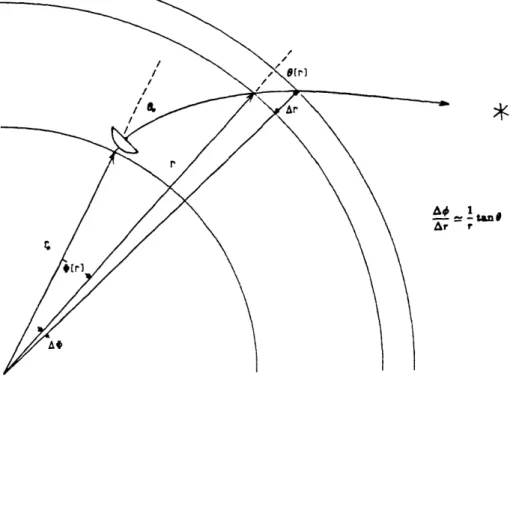
about the center of the earth. In other words, we assume that the earth is a sphere, and that the properties of the atmosphere surrounding the sphere depend only on the radial distance. The explicit solution will lead to the familiar Snell's Law for spherical refraction, and to the "ray-trace" equations for a spherically symmetric atmosphere.

(Although there is a very simple method for solving this particular problem based on Snell's Law for planar refraction, we will elicit the answer the "hard way" for

illustrative purposes.)

We first write down the path-length differential ds in (1.2.1) in terms of the spherical coordinates and X defined in Figure 1.2.1:

ds = V/(dr)

_{+ r}

_(d)

_{= dry/1 + r}

_(Y)

_(1.2.2)

where

<,,-

dr

(1.2.3)

The third spherical coordinate does not appear in (1.2.2) because the assumption of

spherical symmetry assures that the ray will always remain in the plane containing the origin of the ray, the vector parallel to the path of the ray at this point and the

origin of the coordinate system, located at the center of our spherical earth (see Figure

1.2.1).

By substituting the expression for ds from (1.2.2) into (1.2.1), we can see that an appropriate Lagrangian. C is

(a,

';

r) = n(r)

/1

+ r

_(')

_(1.2.4)

The Euler-Lagrange equations then reduce to a single equation with the independent variable being the radial coordinate r

d

-

0

dr

d

-Using

£

d [n(r) r2t =] O (1.2.6)

Thus the term in brackets is a constant. In order to determine this constant, let us first

determine an expression for '. Figure 1.2.1 also shows the geometry which results

from the ray traveling from its position at (r,

0)

formed whose sides are of length r,r + Ar, and As, and whose corresponding opposite angles measure 0 - Ab, r - 0, and AO, where 0 is the angle between the radial vector

and the tangent to the ray at the point (r,

4).

sin( - A) _ sin (1.2.7)

- r+0r

(1.2.7)

r

r + Ar

Both sides of (1.2.7) can be expanded to first order in Ar and AO to yield

9[r]

1

-ta

!7 t

Figure 1.2.1. Geometry for the solution of the Euler-Lagrange equation for a spher-ically symmetric atmosphere.

Solving for AO gives

Ar

r

By taking the limit as Ar -- O0, we obtain the expression for ':

AO 1

'E rlim

-= -tan

(1.2.10)

Ar--O Ar r

Solving (1.2.10) for sinG gives us something which looks very much like the constant term in (1.2.6):

rq~'(r)

_{r5(r) -sin}

_(1.2.11)

v1 + r2(') 2

Substituting sin 0, then, into the constant term in (1.2.6) yields

n(r)rsin (r) = constant = n(ro)r, sin 0(ro)

(1.2.12)

where r is a reference radius. The equation (1.2.12) is Snell's Law for spherical refraction. Using this equation we can write integral expressions for the electrical

path length Le

Le =|

de

ro _/n 2_e2

-n2r2 sin2 0o

and the position angle O(r)

+(r) = nro sin O 0 d1 (1.2.14)

*

e

/n2e2-

n2r

_sin

₀

where in (1.2.13) and (1.2.14) no = n(r,), Oo = (ro), and we have assumed that

the integration begins at ro. The equations (1.2.13) and (1.2.14) are the ray-trace equations for a spherically symmetric atmosphere.

The delay equation (1.1.2) for a spherically symmetric atmosphere can also be written in integral form, using (1.2.13), as

o00 Ta = d ne(n - 1)

/n22

-

nr2 sin

The final integral on the right-hand side of (1.2.15) is the difference in ray paths; Of

is the "true" zenith angle. This integral converges because n -- 1 as -+ oo.

The formulas for the propagation delay which are used in VLBI data analysis are

based on approximations to (1.2.15). The accuracies of these approximations depend

critically on the behavior of the refractive index in the atmosphere. Therefore, before presenting the formulas for the propagation delay, we will discuss the properties of the radio refractive index of moist air. The formulas based on (1.2.15) will then be presented in Section 1.4.

1.2.ii The refractivity of air

Both the general delay equation (1.1.2) and the delay equation for a spherically symmetric atmosphere (1.2.15) contain the term n - 1. For radio wavelengths, the

refractive index n of the atmosphere differs from unity by less than one part per

thousand. Because n- 1 is so small, it is convenient to introduce the refractivity N

defined by

An important feature of the refractivity is that it is a quantity which for linear media depends linearly on the density of the dielectric medium, all other conditions being

constant. (A linear medium is a medium for which the electric susceptibility is

inde-pendent of the applied electric field. The following arguments also hold for media for which the response is for practical purposes linear due to the weakness of the applied

electric field.) To see why this is so, recall that the response of a linear dielectric

medium to an applied electric field E can be written in terms of the polarization P

per unit volume [Jackson, 1975] as

P = E

(1.2.17)

where X is the electric susceptibility of the medium, which may vary in space. (X is unitless and equals zero for vacuum.) Clearly X depends linearly on the density of

the medium, for if the applied electric field remains constant and the density doubles, say, then surely the dipole moment per unit volume must double. Recall that the susceptibility is related to the dielectric constant by

= 1 + 4rX (1.2.18)

where = 1 for vacuum. The dielectric constant is also related to the refractive index by the Maxwell equations for propagation in a macroscopic medium [Jackson, 1975],

which yield the relation

where p, is the permeability of free space ( = 1 for vacuum). For a medium, such as

the atmosphere, with /z 1 and n - 1, (1.2.18) and (1.2.19) yield

-n2 - 1 - 2(n - 1) 4rX

(1.2.20)

Thus the refractivity N is proportional to the electric susceptibility, and therefore also to the density. An approximate expression relating N to the density and temperature

of the medium is given by Debye [1929]

N=

+ B )

(1.2.21)

where A and B are constants which vary for different molecular species, and T is the absolute temperature. The first term on the right-hand side of (1.2.21) arises from the induced polarization (also known as the displacement polarization) of the molecules, and the second term arises from the orientation effect of the applied electric field on the permanent electric dipole of the molecules. If the molecule has no permanent electric dipole moment, B = 0. The derivation of (1.2.21) can be done rather simply, using a semi-classical scheme, or it can be done quantum-mechanically, which derivation is beyond the scope of this thesis. However, by far the most important feature of (1.2.21)

is the dependence of N on the density. Because of this relationship, the refractivity of

a mixture of q species is

N

E-

Ai +

-

)Pi

(1.2.22)

where Ai and Bi are the refractivity constants for the ith constituent, and Pi is its

Although the atmosphere is a mixture of many gasses, it is usual to consider it as being made up of but two: the "dry" gasses, and water vapor. In the following, we

show why this is possible. We will then present experimental determinations for the

refractivity constants for moist air.

1.2.iii The dry atmosphere

The atmosphere of the earth is a mixture of gases and aerosols which maintain a proximity to the earth due to gravitational attraction. The major constituents of

the dry atmosphere are shown in Table 1.2.1. Of considerable importance in this work

is the relative number densities, or fractional volumes of the constituents of dry air. The fractional volume fi of the it h constituent in a mixture of q species is simply the

ratio of the number (or number density) r7i of molecules of that species to the entire number (density) of molecules of all species:

i q17i (1.2.23)

Z ok

k=1

For an atmosphere in hydrostatic equilibrium, we would expect the heavier species

to "sink" to the bottom, and if so the fractional volumes of the various atmospheric

constituents would be a function of height; his will occur only if diffusion is a major source of vertical transport. Below about 90 km, however, mixing processes dominate

over diffusion, so that the mixing ratios of the dry constituents can be treated as being

constant below that height [Colegrove et al., 1965]. (At this height the pressure is about 2 x 10- 3 _{mbar, or about 2 x 10}-_{6 of surface pressure, which for our purposes is to say}

over the surface of the earth. The size of the departures from homogeneity can be seen from the third column of Table 1.2.1. The entries in this column are a measure of the variability of the respective dry constituents, taken from Glueckauf [1951], expressed

in terms of the fractional volume. As one can see, the variabilities of the fractional volumes are very small.

That the fractional volumes of the constituents of dry air are nearly constant is

very useful. It allows us to treat the dry atmosphere as a single gas with molar mass Md given by

8

Md

fiMi

(1.2.24)

i=l

where the sum is carried out over the eight constituents of dry air listed in Table 1.2.1

and the Mi are the molar masses, also listed in Table 1.2.1. A "sigma" for Md, based on the variabilities given in Table 1.2.1, can be calculated approximately by ignoring

the correlations between the variations in the fractional volumes. This approximation

gives

8

t2h

= EZMiai

(1.2.25)

i= 1

where the ai are the (unitless) variabilities listed in Table 1.2.1. From (1.2.24) and (1.2.25) and Table 1.2.1 we can easily compute that Md = 28.9644:i±0.0014 kg kmol-1.

In the following, we will use the fact that the fractional volumes of dry air are constant, and combine all the constituents of dry air together in creating a formula for the refractivity of moist air. We will then present experimental determinations for the values of the refractivity constants.

Table 1.2.1

Primary Constituents of Dry Air

Variability

and Their

Molar Fractional Standard Deviation

Weight Volume for

Constituent kg kmol-l (Unitless) Fractional Volume

N₂ 28.0134 0.78084 0.00004 02 31.9988 0.209476 0.00002 Ar 39.948 0.00934 0.00001 CO2 44.00995 0.000314 0.000010 Ne 20.183 0.00001818 0.0000004 He 4.0026 0.00000524 0.00000004 Kr 83.30 0.00000114 0.0000001 Xe 131.30 0.000000087 0.000000001

1.2.iv The refractivity of moist air

In the previous section, we saw that it is possible to treat the fractional volumes of dry air as being constant. We can now write down the expression for the refractivity

of dry air. Let us write the refractivity Nd of dry air, from (1.2.22) as

8

Nd

Aipi

(1.2.26)

i=l

We have set Bi = 0 for all the dry constituents since none of these constituents

possesses a permanent electric dipole moment. Treating the mixture of dry gasses as a single species, we should also be able to write Nd as

Nd = Adpd (1.2.27)

where Pd is the density of dry air (i.e., the sum of the constituent densities of dry air). The constant Ad is, from (1.2.26) and (1.2.27) defined by

E Aipi 8 8

P i= l Pd

Ad =Ad AifiPdM (1.2.28)

Since Md and the fi are, as we have seen, constant, (1.2.28) shows that Ad is constant

and that the dry constituents combined can be treated as a single gas in the refractivity formula. We may therefore write the refractivity of moist air as

N = klRdPd + k

Rpv, + k

Rv

(1.2.29)

Here Pd is the density of the dry air mixture and Pu is the density of water vapor.

The various A's and B's have all been expressed as kl, k2, and k3. The specific

(1.2.29), since they can be absorbed into any constant; we have included them however in keeping with the conventional values and dimensions in which k, k2, and k3 are presented. Again, note that no permanent-dipole term appears for dry air.

The values for kl, k2, and k3 in (1.2.29) must be determined experimentally. (Although in principle expressions for these constant could be determined from theory,

in practice the theoretical expressions themselves would contain parameters which are

unknown and would have to be determined from experiment.) The method used to determine the constants is to measure the resonant frequency of a cavity into which a known amount of gas has been introduced. This frequency is compared to the resonant

frequency for the evacuated cavity, and the refractivity is calculated [Boudouris, 1963; Essen and Froome, 1951] using

g

Ut

=n-

1

(1.2.30)

Vvt

where vv, is the in vacuo resonant frequency and vg is the resonant frequency with the

gas. For dry air, the dependence of the refractivity on density yields kl. For water

vapor, the dependence on temperature must be used to separate k2 and k3.

Table 1.2.2 contains a partial list of experimental determinations of the constants

in the refractivity formula. A full list of determinations dating back to 1932 appears in

Bean and Dutton [1966]. The precision with which the constant kl (dry air) has been determined is about 0.03% of its value, while the constants k2 and k3 (water vapor) have been determined only to about 8-15% and 1% of their respective values. The

k2 and k3from any single experiment are correlated. This correlation, of course, tends to inflate" the inherent uncertainty of the determination of these constants.

Realizing that the correlation between the estimates of k2 and k3 was a limi-tation, Thayer [1974] attempted to reduce its effect by constraining the value of k2 to its optical value. (At optical frequencies, the k3 term does not appear and the

k2 term can therefore be determined with greater precision.) Through the breaking of the correlation, the uncertainty in the k3 term was reduced accordingly. Thayer's

values for k2 and ks3 are also shown in Table 1.2.2. It is interesting to note that the

predicted value for the radio value of k3, based on using the optical value for k2, is quite close to the experimental determinations of k3 in the radio range. While this result does not prove that extrapolation from the optical range to the radio range

for k2 is correct, it does mean that Thayer's values are probably no worse than the experimental determinations.

Hill et al. [1982] have criticized Thayer's extrapolation from the optical from a

theoretical view. They claim that this extrapolation ignores the contribution of the

infrared (vibrational) resonances. Based on this criticism, Hill et al. use tables of the

infrared spectra of water vapor to calculate this contribution; these calculated values

for k2 and k3 are shown along with the others in Table 1.2.2. The "uncertainties"

associated with the values from Hill et al. reflect the fit of the theoretical model expressed by (1.3.21) to the calculated values, as reported by Hill et al.. It can be seen that these values for the refractivity coefficients are significantly different (in terms of

the experimental uncertainties) from the experimental values. Hill et al. are unable to

Table 1.2.2

Determinations of Refractivity Constants

Reference Frequency kl k2 k3

GHz K mbar- 1 K mbar - 105 K2 _mbar - 1

Essen & Froome [1951] 24 77.68 ± 0.03 64.7 3.72

Birnbaum & Chatterjee [1952] 9-25 71.4 ± 5.8 3.747 ± 0.03

Boudouris [1963] 7-12 77.64 ± 0.08 72.0 ± 10.5 3.75 ± 0.03 Thayer [1974] < 20 77.60 ± 0.02 64.8 ± 0.1 3.776 i 0.004

values. This conflict will probably remain with us until more accurate studies of the refractivity of water vapor at long wavelengths are undertaken.

1.2.v Dispersion in the atmosphere

The formula for the refractivity of moist air given in (1.2.29) contains no depen-dence on frequency. A formula for the refractivity which inclndes dispersion can be written as [Liebe, 1985]

N(v) = No + No () + Nv(v) + N

(v) + N.(v) + N (v)

(1.2.31)

In the above equation, No is the nondispersive term of the refractivity, given by

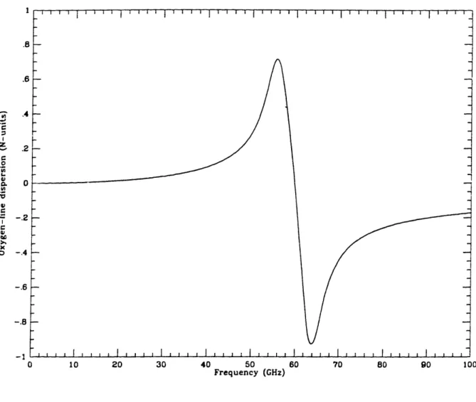
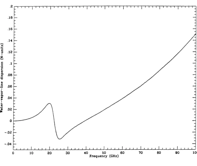
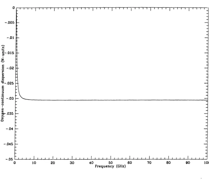
(1.2.29). The terms No2(v) and Nv(v) are the contributions of the anomalous disper-sion due to the oxygen and water-vapor lines, respectively. The terms N 2(v), Nv (v), and Ne (v) are the contributions of the continuum dispersion of dry air, water vapor,

and liquid water, respectively.

Formulas for each of the dispersion terms can be found in the Millimeter-wave Propagation Model (MPM), outlined in Liebe [1985]. Figures 1.2.3-1.2.6 show the

individual contributions to the dispersion from the MPM , in the range 0-100 GHz and for a total pressure of 1013.25 mbar (1 atm), a temperature of 300 K, and a relative humidity of 50%. Figure 1.2.7 shows the total refractivity for these parameters, and

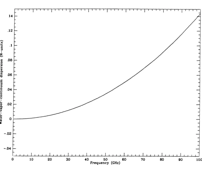
for a liquid density of zero. The largest dispersion in this range is due to the 60 GHz oxygen line, and deviates from the zero-dispersion value by about 1.5 N-units, or about 0.5% of the nondispersive refractivity. Below 30 GHz, the dispersion is less than 0.04%

of the nondispersive value, and is due not only to the water-vapor resonance, but also

to the tail of the 60 GHz oxygen resonance and the water-vapor continuum dispersion.

Although the dispersion below 30 GHz is small, it is not negligible with respect

to the uncertainty with which the refractivity is known (see Section 1.2.iv). The dry refractivity constant kl is known to about 0.03% of its value. We will continue to use the nondispersive formula for the refractivity, with the understanding that it may need appending as per the MPM.

Figure 1.2.8 shows the dispersion due to liquid water from the MPM, for a liquid water density of 0.5 g cm-3 and a temperature of 280 K. This density is typical for clouds of thickness between 200 and 600 m [Decker et al., 1978]. No existing formulas for the atmospheric propagation delay includes the effects of liquid water, since it is difficult to estimate the amount of liquid water except by remote sensing. From Figure

1.2.8, hovever, we can see that the zenith propagation delay through a cloud with this

temperature and liquid density and a thickness of 500 m is approximately 3.5 mm for a frequency of 8 GHz. For a slant path of 10° elevation, the delay through such a cloud is approximately 2 cm. If we compare this delay to typical group-delay uncertainties of about 1 cm, we can see that this delay is not in general negligible. We will discuss

this topic further in Chapter 5.

We have now completed our review of the properties of the refractive index at

microwave frequencies, and turn to the presentation of formulas for the propagation

de-lay, and the effects of errors in these formulas on the estimation of geodetic parameters

from VLBI data. However, preliminary to this presentation, we will review a number

20 30 40 50 60

Frequency (GHz) 70 80 90 100

Figure 1.2.3. Contribution to the dispersive refractivity of 02 resonances, primarily

those near 60 GHz, calculated from the MPM (see text). The values of the relevant thermodynamic parameters were pressure P = 1013.25 mbar and temperature T =

300 K. I .8 .6 z o,. Do I. c 0. Cx x 0o .4 .2 0 -. 2 -.4 -. 6 -. 8 -1 0 10 - - - s - - - -_ -_ .

10 20 30 40 50 60

Frequency (GHz)

70 80 90 100

Figure 1.2.4. Contribution to the dispersive refractivity of H20 resonances, calcu-lated from the MPM (see text). The values of the relevant thermodynamic parameters were pressure P = 1013.25 mbar and temperature T = 300 K, and relative humidity

RH = 50%.

r~~~~~~~~~~~~~~~~~

D , i,, I,,,, I,,,, I, | a | I 4 | | | I | | ' | I ' ' ' ' I ' ' '' ' I ' ' ' ' I ' ' ' '_

i f

-10t-

2

Figure 1.2.5. Contribution to the dispersive refractivity of the 02 continuum,

calcu-lated from the MPM (see text). The values of the relevant thermodynamic parameters were pressure P = 1013.25 mbar and temperature T = 300 K.

-.005 -. 01 r-.015

z

10 20 30 40 50 60

Frequency (GHz)

70 80 90 100

Figure 1.2.6. Contribution to the dispersive refractivity of H20 continuum, calcu-lated from the MPM (see text). The values of the relevant thermodynamic parame-ters were pressure P = 1013.25 mbar, temperature T = 300 K, and relative humidity

RH = 50%.

,,,,I

I

I IA

j i,,,,,,I

, ,I,,,,

,III,,

,,I,

-. 02 -. 04 0 .. . . ._ · r · ~ 1 · · _· 1 _ · · _ · ~ ~ ~ ~ _- - . . . . - - - - --I b I -- --I

,,,I I . . .. I I, , ,

0 10 20 30 40 50

Frequency (GHz)60 70 80 90 100

Figure 1.2.7. Total refractivity, from the the MPM (see text). The thermodynamic

parameters used were those used for Figures 1.2.3-1.2.6.

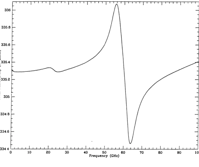
336 335.8 335.6 I 335.4 z ,. a, '-334 8 334.6 334 4 · _ ._ . . . _ or . . A . . . . - . - 1 . I · . . . . . I I I I I I I I I I .I I . . . I I I I I I I .I 1 . . I I 1 1 I I I 1

I

I h f I I f I I I i l , I h I I If I

0 10 20 30 40 50 60

Frequency (GHz)

70 80 90 UU

Figure 1.2.8. Contribution to the dispersive refractivity of the liquid water contin-uum, calculated from the MPM (see text). (This contribution is not included in the

calculation for Figure 1.2.7.) Cloud-like conditions of T = 280 K and pi = 0.5 g cm - 1 were used. .12 .1 .08

7

1.3 Modeling the atmospheric delay: some definitions

In this section, we will define several terms which are often used when modeling

the atmospheric propagation delay. These are zenith delay, mapping function, and wet and dry delays.

1..i The zenith delay

The zenith delay is defined to be the atmospheric propagation delay (1.1.2) for

a signal arriving from the zenith direction. Although in general the path of the ray

arriving from this direction may be curved, for a spherically symmetric atmosphere we find that the ray path is a straight line, because the path strikes the lines of equal

refractive indices normally. We also obtain this result immediately from (1.2.14), which is the equation for the position angle. The delay equation (1.2.15) for a spherically symmetric atmosphere reduces to

ra

j

This equation can be rewritten in terms of the height z above the earth, z = r/ - rt, as

=

j

where N(z) is the refractivity defined in (1.2.16). The superscript z indicates the zenith delay. Even though (1.2.15) is impossible to integrate analytically, as noted

below this equation, it is possible to find analytical, closed-form solutions for the

1..ii The mapping function

In the section defining the zenith delay we saw that the integral solution for the

delay (1.2.15) had a relatively simple form for the delay in the zenith direction (0o = 0). The only other realistic form for the refractive index which has such a simple solution

is N(z) = constant. Then again there is no bending, and the delay as a function of

elevation c can be written in terms of the zenith delay r, and for a plane-parallel

earth, as

rc,(E) = csc E (1.3.3)

In (1.3.3), the function csc is known as the "mapping function" because it relates the zenith delay to the delay at all other elevations. In this example, the mapping function

contains no dependence on azimuth because of the assumption of spherical symmetry. The csc E mapping function is usually referred to simply as the cosecant law." The earth's atmosphere is described by the cosecant law to some approximation. In fact,

(1.3.3) motivates us to write the atmospheric delay as

Ta(E) = r7. m(E) (1.3.4)

where m(e) is the true mapping function, which as we noted is only approximately described by the cosecant law. Because overall the refractive index decreases with

height, and because the earth is approximately spherical, the true mapping function

will nearly always be less than the cosecant of E, for all c. (The exceptions to this rule

result from horizontal variations of the refractive index.)

It is important to remember that (1.3.4) defines the mapping function m(E). Other kinds of mapping functions can be defined. For instance, the grouping of the

right-hand side of (1.1.2) into two terms might motivate us to define two functions: the mapping function, which scales the zenith delay, and an additive "geometric delay" g

T.(E) =

-m(E) + (E)

(1.3.5)

Such a form has been suggested, for example, by Elgered and Lundqvist [1984]. Other

definitions are, of course, possible. The form one uses depends on the manner in which one attempts to find a formula for the mapping function, and the manner in which one will ultimately use the mapping function. For example, as discussed in Chapter 2, an

instrument known as a water-vapor radiometer (WVR) is in principle able to determine

the "wet" path delay (which will be defined below) along the line-of-sight. Thus, a model combining the "dry" delay and the wet" delay determined from WVR data would have the form

ra(E)

=

r

*.

m(e) + TWVR

(1.3.6)

where Tr is the zenith "dry" delay and rwvR is the line-of-sight wet path delay

deter-mined by the WVR.

In the next section, we will describe in more detail what we mean by wet" and "dry" delays. The definitions for these terms are important, for as we have seen these

terms also define the mapping function.

1.S.iii The wet and dry delays

Terms like wet delay" and "dry delay" are often used, but are seldom defined

carefully, and frequently not at all. This state of affairs is unfortunate, since there

different terms for both the refractivity and the delay. We will give the definitions which will be used in this thesis, but they are not universal. We believe, however, that they are "best" in a sense that will be discussed below.

The definitions of "wet" and "dry" refractivities are unambiguous, because it is possible to write an expression for the refractivities of dry air and of water vapor. In

terms of the constants kl, k2, and k3 introduced in Section 1.2.iv, we have

Nd = klRdPd (1.3.7)

Nv= kR= p

+

_T

Let us examine the zenith delay. Equation (1.3.2) can now be written

r~ = 10- 6 dz Nd +lO 10- 6 dz Nw (1.3.9)

It seems obvious to call the first term on the right-hand side of (1.3.9) the dry zenith

delay, and the second term the wet zenith delay. These definitions become inconve-nient, however, when one attempts to derive formulas for the zenith delay. The reason for this inconvenience is that it is necessary to know the profile of the density of dry air

for the integration of the dry refractivity, and it is also necessary to know the profile of the density of water vapor for the integration of the wet refractivity. On the other hand, it is possible to estimate the integral of the total density without knowing its specific profile. This ability stems from the equation of hydrostatic equilibrium, from

which we obtain

where Po is the pressure at the base of the vertical column, p(z) the total density

(specified here and hereafter by the omission of any subscripts), and g(z) is the

accel-eration due to gravity. Because gravity varies only slightly over the effective range of the integration in (1.3.10), we can expand g(z) to first-order in z with negligible error,

and write (1.3.10) as

f00 (00

Po = g dz p(z) +g dzz p(z) (1.3.11)

where g' is the derivative of g with respect to height evaluated at the surface. We can

rewrite the second integral in terms of the altitude HC of the center of mass of the

vertical column, which by definition is

H -fo dz z p(z)

H

_

fo dzzp(z)

(1.3.12)

fo dzp(z)

Substitution of (1.3.12) into (1.3.11) yields

Po = (go + gHc)

dz p(z)

(1.3.13)

Although we have not examined the accuracy of (1.3.13)-this is discussed in

Ap-pendix A-the implication of this equation is clear: it is possible to estimate the integral of the total density using the pressure at the base of the vertical column. This result prompts us to rearrange (1.2.29) in terms of the total density, and the remaining water vapor terms:

We will now define the "dry" zenith delay to be

.r

= lO0-6klRd

(1.3.15)

= 10-

_{klRd(go +}

_g'Hc)

_Po

and the "wet" zenith delay to be

=

dz

2

-Md kl+ T(z)]

(1.3.16)

Several things should be pointed out about these definitions. Firstly, they are just that:

definitions. For other applications, it might be convenient to have other definitions.

One might disagree with the term "dry" for the quantity defined in (1.3.15) because it

depends on the total density. However, this term is a "dry" zenith delay in the sense

that if it were known that the atmosphere contained no water vapor, r would still

be defined by (1.3.15), because it is "parametrized" by the total pressure. It is not a

"dry" zenith delay in the sense that the mean molar mass of the atmospheric gas, the

density of which is p, is not equal to the molar mass of dry air.

Let us now move on to the propagation delay for directions other than the zenith.

In terms of the refractivity, we can write the delay equation (1.1.2) as

ra

=

10-6

ds N(s) + [

ds

ds

(1.3.17)

atm atm vac

If we express the refractivity not in terms of the wet and dry refractivity, but in terms of the total density and water-vapor density as in (1.3.15) and (1.3.16), (1.3.17)

becomes

ra = 10-6klRd f~ ds p(s)

tm

+ 10-6RV

ds 2-

tkl

+

) P

(1.3.18)