Thermal and hydraulic aspects of the KTB drill site

(1)

Geophys. J . Int. (1996) 124,756-172

Thermal and hydraulic aspects

of

the KTB drill site

T. Kohl and L.

Rybach

Institut f u r Geophysik, E TH-Honggerberg, CH-8093 Zurich, Switzerland

Accepted 1995 September 21. Received 1995 August 17; in original form 1994 November 8

S U M M A R Y

The extensive data sets obtained by the KTB drilling project (lithological and structural information, BHT values, temperature logs, rock thermal properties) provide a unique opportunity to construct realistic thermal models and thus to shed light on thermal conditions in the upper crust. Our numerical simulation study, a Swiss contribution to the German KTB drilling project, aims to understand the steady-state thermal and hydraulic field in the surroundings of the KTB. The simulations consider state-of-the- art petrophysical aspects relevant to deep, pressurized, high-temperature structures and were performed on discretized 2-D/3-D finite-element meshes that contain topography, geological structures and hydrogeological features.

Our analysis of the KTB temperature field suggests three zones of particular geothermal settings: a low-heat-flow zone in the uppermost layers with a transition to high heat flow at 500 m depth; the underlying region accessed by the borehole with its characteristic uniform gradient; and the mid-lower crust that must be responsible for the high-heat-flow regime at the KTB site. The two first zones are treated in the present paper.

A

3-D thermo-hydraulic model was set up in order to evaluate the first

2000

m, including the uppermost 500 m low-heat-flow zone. This model incorporates the complex geological information from the KTB pilot hole and topography-driven fluid flow. The lateral boundaries of the model were carefully chosen by analysing the flow pattern within a large, regional 3-D domain. The drilled section is analysed by a 2-D model using the available structural information. Due to dominating refraction effects, a careful temperature gradient analysis has to be carried out for such steeply dipping, anisotropic structures. Both models indicate a thermal regime dominated by diffusive heat transfer. Hydraulic flow seems to be important only for the uppermost (- 400 m) part of the drilled depth section; our simulations do not support significant fluid circulation at greater depths. In the drilled section the rather uniform gradient and the pronounced vertical heat-flow variations can now be explained.

Finally, the potential and the limitation of the analysis

of

heat flows and temperature gradients are demonstrated. Heat-flow interpretations are conclusive only for nearly horizontally layered, isotropic geological units. In steeply dipping and anisotropic formations the heat-flow field is perturbed over a large distance (> 1 km) around the point of interest. In such geological units only the temperature gradient interpretation can provide reliable information on the surrounding material.

Key words: heat flow, numerical modelling, thermal and hydraulic field, upper crust.

depth of 9101 m in 1994 September. As a Swiss contribution to the German KTB drilling project, the numerical simulation study described here aims to understand the geothermal field in the surroundings of the KTB site. The work has been performed in co-operation with several KTB investigators.

The various data sets collected and analysed in the KTB field laboratory for the VB and the HB, as well as investjgations in the surroundings, show the complex structure of this area. 1 I N T R O D U C T I O N

The main stage of the German Continental Deep Drilling (KTB) project started in 1987 with the objectives of determin- ing the physical conditions and revealing the geological structures in deep crystalline rock. First, a 4000 m deep pilot hole (VB) was drilled, accompanied by large-scale data acquisition. After that the main hole (HB) was sunk, reaching its final

(2)

Thermal and hydraulic aspects of K T B 757

The main tectonic unit at the KTB location is the Hercynian Zone of Erbendorf-Vohenstrauss (ZEV). The centre of this zone is characterized by steep, SW-dipping, alternating gneissic and metabasic rock units. To the W, there are Mesozoic sedimentary cover rocks and to the NE, large granitic intrusions are found. Seismic sections and borehole data show eastwards dipping cataclastic joint zones that can be correlated with surface topography. A detailed geological description to

the KTB site is given by Emmermann (1989).

The intention of the present study is to condense and integrate the available information into a numerical model that is based on state-of-the-art petrophysical aspects relevant to deep, pressurized, high-temperature structures. The geothermal observables such as temperature, temperature gradient, thermal conductivity, heat production and the derived quantity heat flow represent the basis of our interpretational steady- state approach. In addition to assumptions about thermal parameters, assumptions about permeability distribution in crystalline rocks had to be made. A correct choice of parameters should yield a calculated temperature profile, a vertical temperature gradient and a heat-flow density in agreement with the observed values. In particular, the dependence of the data on strongly dipping, alternating gneissic and metabasic geological units has been addressed.

In the following section a summary of those factors that are likely to be relevant to the hydro-thermal situation at the KTB site will be given.

2 G E O T H E R M A L A N D H Y D R A U L I C SITUATION

The thermal parameters measured in the KTB field laboratory provide an enormous data base on thermal conductivity and heat production. The petrophysical investigation differed in the VB and the HB operations: measurements could be performed during the VB phase on core samples, whereas only data from cuttings are available from the HB phase.

Besides the excellent thermal laboratory measurements on rock samples, only very poor temperature data are available from borehole measurements. The last complete temperature log in the VB was measured about 250 days after the drilling stopped. Because considerable activity took place in the borehole during these 250 days, deviations of this log from the conditions of the undisturbed thermal field must be expected. A second VB temperature log was conducted one year later, but only down to a depth of 2000m, where at that time a packer plugged the borehole. During the drilling phase of the HB, the most reliable temperature measurements indicating the undisturbed temperatures were obtained from BHT measurements made at approximately 1000 m intervals.

The heat-flow values calculated from gradient and vertical thermal conductivity data (Huenges & Zoth 1991) show a peculiar feature: low values of around 0.05 W m-' occur in the upper 500m, but at greater depths the values rise to 0.08-0.09 W m-'. Below 1200 m, a nearly uniform thermal gradient of 0.028 K m-I was derived from BHT measurements and temperature logs for the entire drilling depth. Correspondingly, high temperatures have been encountered at greater depth: a BHT measurement at 81 10 m indicates 229 "C. Obviously, the temperature field at the KTB is strongly influenced by the geological structure, since the heat will preferentially flow along the near-vertical, better-conducting

gneissic formations with strongly anisotropic thermal conductivity (3.0 W m - l K-' perpendicular to the foliation and 3.6 W m - l K-' parallel to the foliation; see Huenges & Zoth 1991), rather than within the low-conductivity, isotropic meta- basites (2.5 W m - l K-l).

The objective of heat flow modelling in the surroundings of KTB is to combine the laboratory data sets with standard geothermal simulations described in, for example, Chapman & Furlong (1992). The observation of different heat-flow regimes at depth suggests that both the diffusive and the advective component of heat transport has to be addressed and evaluated. The following three zones in the KTB terrain are of particular geothermal interest:

(1) the upper 2000m, to investigate the uppermost low- heat-flow zone within a high-heat-flow regime;

(2) the drilled part of the upper crust down to 9000m, to explain the appearance of a uniform temperature gradient along with a strongly varying heat flow;

(3) the mid-lower crustal domain, to explain the origin of the generally high-heat-flow regime.

The appearance of a low-heat-flow zone in the upper 500 m within a generally high-heat-flow regime has been extensively studied and discussed in the literature. The low-heat-flow zone is in agreement with heat-flow determinations that were performed in shallow boreholes for site investigation studies in the surroundings of the KTB. These boreholes indicated low values in the range of 0.04t00.075 Wm-', and led to erroneously low temperature predictions at depth (Burkhardt

et al. 1991). The considerations of Jobmann & Clauser (1994) and Rybach (1992) are important for the characterization of this feature. According to these authors, the low-heat-flow zone at shallow depth could be due either to palaeoclimatic effects, or to the influence of hydraulically driven advection or to a combination of both.

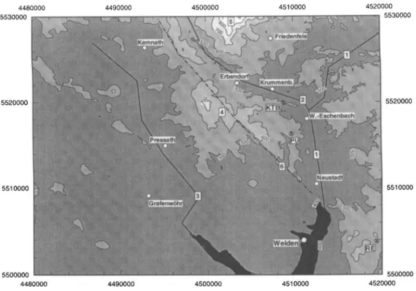
A detailed study of the appearance of a low-heat-flow zone in a regional high-heat-flow regime is important since it can possibly prevent future misinterpretations of heat-flow data from shallow boreholes. The present study focuses on this problem by using a regional, combined thermo-hydraulic 3-D model of the uppermost 2000 m that incorporates topography effects as possible driving mechanisms for advective transport. Topography represents the strongest factor influencing the near-surface hydraulic pressure field. A topographic map of the vicinity of the KTB (altitude 505 m) within a 10 km radius is shown in Fig. 1. It can be seen that the altitudes range from 950 m in the Fichtelgebirge to 400 m in the lower plains of the sedimentary cover rocks. The significance of hydraulic impact on the thermal field was highlighted recently by Jobmann & Clauser (1994) who performed 2-D calculations along a NE-SW profile running through the KTB site. They also identified a hydraulically influenced temperature field at various other, shallower boreholes located in the surroundings of the KTB. Based on 1-D Peclet number analysis they concluded that the boreholes located in crystalline rock (i.e. NE of the Frankonian Line) are characterized by downwards-percolating fluids, whereas the only available borehole west of the Frankonian Line is characterized by rising fluids. After cor- recting for the hydraulic effect, all boreholes yield a higher basal heat flow than the raw data.

In the present paper, this uppermost zone is evaluated by means of a detailed 3-D model. It is intended to elucidate

(3)

758 T. Kohl and

L.

Rybach

Figure 1. Topographic situation around KTB (isolines in m.a.s.1.). The coordinates correspond to the German coordinate system (in m). The topography is characterized by lower plains in the south and south-west and by increasing heights in the north of the KTB. The main features on the map are indicated by numbers. 1: the Waldnaab river; 2 the Fichtelnaab river in the valley near the KTB location which joins the Waldnaab 3: the Haidennaab river with sedimentary bedrock; 4 the Kiihberg; 5: the heights of the southern Fichtelgebirge; and 6 the Frankonian Lineament (dashed line) that separates the crystalline block in the east from the SW-situated sediments. All rivers discharge into the Danube, about 100 km south of Weiden. Also labelled on the map are the drillholes Pullersreuth (PU) and Remmersberg (RE), which were sunk during the site investigation study (see Burkhardt et al. 1989).

thermal and hydraulic effects by means of a detailed geological and topographic description.

At greater depths, the hydraulic flow field seems t o be

decoupled from near-surface domains (Kessels, Kiick & Zoth 1992) and influenced by fluid-density variations due t o higher salinity. Huenges (1993) showed that pressure measurements can be interpreted as a n increase of density with depth, up to 1200 kg m-3 a t 3000 m. The significance of pressure variation due to a permeability variation remains uncertain, since borehole permeability measurements in the KTB d o not indicate any significant variation with depth. The difference between laboratory-scale and large-scale measurements from the same depth extends over several orders of magnitude. Laboratory measurements o n samples from intact rock show permeabilities of around lo-'' m2; a hydraulic communication test over the 200m distance between VB and HB revealed values of the order of

The second zone to be simulated represents the thermal field of the upper crust (< 10 km). It accounts for the complexity of the local geological structures. In particular, the thermal effect of the steeply dipping geological units was investigated. The drill-core data from the VB also revealed the angle of dip of the geological units, as illustrated in Fig. 2. In the upper 2000 m, which has the steepest foliation, dips of u p to 90" can be found. Below is a zone with a rather shallow dip angle, and at around 3000m the foliation dip increases again to about 60". Simple, steady-state diffusive heat transport for the main part of the drilled section is assumed in this paper in the

m2 (Kessels et al. 1992).

Foliation Dip Angle VB

-500 -1 000 -1 500

-

_E 5 -2000 n I a, -0 -2500 -3000 -3500 -4000

o

20 40 60

ao

dip angle

Figure 2. Dip of the geological units in the 4000 m deep VB drillhole.

(4)

Thermal and hydraulic aspects of K T B 159

investigation of this feature. Our approach is to consider further heat transport mechanisms only if a successful diffusive simulation cannot be performed. The geological model of the upper crust by Hirschmann (1993) is the basis of our study.

The simulation of thermal transport at greater depth (mid- lower-crustal domain), and thereby the origin of the high heat flow, must necessarily be more speculative. The Eger Graben

(25 km NE of the KTB) represents a young tectonic pertur-

bation and therefore a possible regional heat source. It is considered to be the junction between the Hercynian Saxothuringian and Bohemian massifs. A deep-reaching fault zone is indicated by the gas content of fluids. Fluids sampled from mineral springs at a fault zone near the SW border of

the Eger Graben have a large portion of mantle-derived helium (Weinlich, Brauer & Kampf 1993). A further indication of mobile crustal fluids causing stress perturbations are seismic swarms with focal depths around 10 km (Dahlheim 1993). The epicentres of these events are located about 20 km from the

KTB near some basalt outcrops, close to the SW border of

the Eger Graben.

Subrecent volcanism is also known to have originated from the Eger Graben. According to Kopeck9 (1986) three eruptions close to the Czech-German border represent the youngest volcanic event, which is dated at 860 ka BP. Radiometric measurements indicate an even more recent age of approximately 260 ka BP (Sibrava & Havlicek 1980). The nearest event to the KTB is located at about 28 km to the ENE. These

volcanic events represent the latest manifestations of several episodes that started in the Early Miocene with the strongest activity some 20-25 Ma ago. The centre of that main episode

was near Roztoky in the central Eger Graben. During the Early Miocene, the activity extended westwards up to the sediments SW of the Frankonian Line. The likelihood of a

thermal influence on the heat flow below the KTB will be evaluated in a separate study. The Eger Graben has already been mentioned by Burkhardt et al. (1991) in an analysis of possible regional heat sources. The present authors are cur- rently investigating this point (see some preliminary results in Kohl & Rybach 1994), so no further discussion will be given here.

Before a quantitative interpretation of the thermal regime in the two uppermost zones is presented, the thermal and hydraulic mechanisms considered, as well as the discretization procedure, will be described

3 T R A N S P O R T M E C H A N I S M S I N D E E P CRYSTALLINE R O C K

The general porous medium approach was applied to treat mass and thermal transport in the realm under consideration. Diffusive thermal transport can be described with the Fourier equation

q = - I V T , ( 1 )

where q is the heat-flow vector, 1 is thermal conductivity, V is the Nabla operator and T is the temperature. Although /z generally is treated as a scalar, anisotropic effects can be approximated applying only the vertical component of thermal conductivity. At the KTB site with its steeply dipping angles (60"-80"), off-diagonal terms of the real second-rank thermal- conductivity tensor are small compared to the vertical component (Azx < I,, and

a,,

< I,,). Furthermore, lateral temperature

gradients are negligible (aT/dz >> aTjax, dT/az >> aT/ay). Thus, the vertical component of the heat flow, yz, which is the only one measurable in vertical boreholes. can be approximated by q = -

-a,,

- aT - ax aT

LT

- I PT -A,, -- . az

For modelling purposes, the value of il in a porous medium can be best approximated from cuttings or cores by applying the geometrical mean between the solid and the fluid phase (Pribnow 1994). If not only diffusive but also advective thermal transport is considered, the thermal energy equation for steady state can be written as

V ( ~ V T ) - [ P C ~ ] ~ V ~ V T + H = O , (3) where

[ p c P l f

is the specific heat capacity of fluid, vd is the Darcy velocity and H is the heat production rate.

The hydraulic pressure field is commonly described by combining mass conservation with Darcy's flow law. Its extended form can be given as follows:

V ( $ [ V h - (Pf - P'JVZ]) =

o,

PfO (4)

where 1-1 is the dynamic fluid viscosity, k is the matrix per-

meability, pfo is the reference fluid density, pf is the fluid density, g is the gravity, V z is the vertical component of the unity vector and h is the hydraulic head. The term

(pf - pfo)Vz/pf, describes the effect due to the density difference between reference density and in situ density.

The physical conditions in deep crystalline rock are different from those near the surface or in the laboratory. This implies that in the above equations the temperature and pressure dependence of fluid and rock properties must be considered. The implications are manifold for a geothermal model in deeper regions of the crust, since several non-linear constitutive relationships have to be taken into account.

The non-linear dependence of the fluid parameters was taken from Phillips et al. (1981), who analysed the behaviour of brines for different data bases. The dependence of rock thermal conductivity on temperature and pressure has been measured by, for example, Buntebarth (1991) and compiled by Clauser & Huenges (1995). A preferred fitting curve for the decrease of conductivity with temperature is a hyperbolic function:

1 ( A

+

B T ) '

i ( T ) = ~ ( 5 )

where A and B are lithology-dependent constants. The para- meter A represents the reciprocal of the thermal conductivity at T= 0 "C. The parameter B, which describes the decrease of with temperature, is also lithology-dependent: samples of higher conductivity show a stronger temperature dependence than those with lower conductivity. On the basis of the data published by Clauser & Huenges (1995), B can be linearly interpolated between a maximum of 3.4 x W m-' for IT=O-C > 3.5 W m-l K-' and a minimum of 3.2 x W m-l for < 2.5 W m-l K-'. For temperatures above 450°C all thermal conductivity data sets occupy a very close bandwidth around 2 W m - l K-'. The pressure dependence is less pronounced: the increase of thermal conductivity with pressure can be as much as 15 per cent at pressures of 10MPa and stabilizes in higher-pressure regimes. The pressure correction used for this work involves a linear increase of thermal conductivity from 0 to 10per cent over the pressure range 0

(5)

160 T , Kohl and L. Rybach

to 10 MPa. Thereafter the conductivity remains independent of pressure.

Although anisotropy is not explicitly treated in this paper, it must be kept in mind that these relationships concern all components of a thermal-conductivity tensor. The general tensorial form of thermal conductivity is the result of a transformation from a local, geological coordinate system into the global coordinate system of the whole domain under consideration. However, in the case of isotropic materials, the thermal conductivity can be treated in scalar form since the transformed structure will again be isotrop'ic.

The rate of heat production depends mainly on the U, Th and K contents. Therefore, granitic lithologies produce more heat than sediments (see e.g. Rybach 1988). U, Th and K are preferentially enriched in the upper crust. The depth profiles of heat production assume an exponential decrease in the mid and lower crust.

4 N U M E R I C A L A N D D I S C R E T I Z A T I O N P R O C E D U R E

The simulation tool used was the 3-D finite-element code FRACTure (Kohl & Hopkirk 1995). Among other features, the program allows steady-state and transient simulations of the coupled hydraulic and thermal processes underground. Special emphasis is given to the treatment of the non-linear temperature and pressure dependence of thermal conductivity. This property is adjusted according to the local temperature and pressure field by the lithology-specific functions mentioned above. Since FRACTure uses a linear solution algorithm, the solution will be approached by iteration. For the type of problems discussed, convergence is reached typically within 10 iterations.

Special emphasis is devoted to the discretization of irregular finite-element networks. Experience shows that automatic mesh generation of arbitrarily shaped bodies nearly always needs successive manual adjustment. Therefore, a special module for the mesh-generating code FRAM was designed. To treat a given domain, a rough finite-element mesh is first descretized manually using all the advantages of a commercial CAD sortware package. In a second step the code refines the mesh automatically. The possibility for insertion of a scanned geological section into the CAD software to give a background pattern for the discretization is a further useful feature. Copying these 2-D discretizations into the third dimension and applying the appropriate material properties yields a full 3-D mesh. Additional tools incorporated in FRAM allow the rotation of these 3-D bodies or the selection of optional cross-sections which can be transposed. The latter option also permits the upper surface of a body to be adjusted to the true topography, or to the shape of an irregular internal geological layer to be represented.

5 S I M U L A T I O N O F T H E U P P E R P A R T OF KTB-VB

5.1 Background and preparatory investigations

The aim of the simulation of the upper 2000 m of the VB was to elucidate the 3-D thermo-hydraulic effects in this zone. This was possible since the VB data base is more complete and

reliable than the HB data base. The thermal effects caused by the strong lateral heterogeneities in the vicinity of the KTB site require considerations in a depth range in which 3-D information is available. This is generally the uppermost part of a borehole since surface considerations can add information from the two horizontal dimensions to the 1-D borehole information. The topography-driven hydraulic flow field and the steeply dipping gneissic and metabasic structures represent first-order lateral heterogeneities. Necessary information on the adjacent geological structures is available from the analysis of core samples and the distribution of geological units on the surface. The characterization of the hydraulic influence in the thermal field requires a special approach since the relevant local hydraulic regime needs to be determined.

Before modelling the thermal regime near the surface, the distribution of thermal conductivity and heat production for the different lithologies was evaluated. The data collection of the KTB field laboratory could be used, but the surrounding materials, including granite, graphitic quartzite and green- stones, also had to be investigated. Therefore, near-surface materials were collected and their thermal conductivity was measured (Medici 1994). An astonishingly high thermal conductivity (higher than 7 W m - l K-') was determined for the graphitic layers of the Wetzldorf sequence located 5 km north- wards of the KTB, which agrees well with the findings of Jobmann & Clauser ( 1994). This unit represents the collision zone between the Moldanubicum and the Saxothuringian that was originally targeted to be drilled in the KTB project. This sequence extends laterally only 3 km in an E-W direction at the surface and has a rather limited thickness. Since it is uncertain whether the graphitic quartzites extend down to greater depths they were not considered in the present study.

The model consists of the following materials: sediments; metabasite; gneiss; and granite. Although known to be anisotropic, the thermal conductivity of the steeply dipping gneissic formations was treated as isotropic. The value of the thermal conductivity was chosen to be the vertical component originat- ing from the mean dip of the gneiss. The diffusive thermal material parameters at a reference temperature of 20 "C and zero pressure of the four materials (sediments, metabasite, intermediate dipping gneiss and granite) used in the 3-D model are shown in Table 1.

Since the objective of the thermal simulation was to explain the measured temperature field by the thermal-conductivity and heat-production structure, the measured values of these parameters were left unchanged. This represents a strong restriction for the fitting procedure, since the measured temperature data should be explainable by two homogeneous

Table 1. Thermal material simulation. Sediments Gneiss steep Gneiss, intermediate Gneiss, near-horizontal Metabasite Granite Mid crustal

properties (at 20°C) for 2-D/3-D Thermal conductivity [W m-' K - ' 2.0 3.3 3.2 3.0 2.5 3.7 3.4

1

Heat production CPW m-31 0.4 1.5 1.5 1.5 0.8 6.0 1.0-0.6 0 1996 RAS, GJI 124, 756-772

(6)

Thermal and hydraulic aspects of K T B 761 materials only (metabasite and steeply dipping gneiss) that

were encountered in the KTB.

Our sequential approach in modelling will be as follows: a regional hydraulic model to define the lateral borders of a refined 3-D model, a local thermal model to investigate a thermal diffusive field, and finally a local thermo-hydraulic model for the evaluation of advective thermal transport. 5.2

The evaluation of the local hydraulic regime requires a model with reliably known lateral boundary conditions. Therefore, a large regional 3-D model was set up extending laterally over the surface indicated by Fig. 1 and a local model was extracted from it. Furthermore a refined accurate thermal-transport calculation can only be performed on a smaller model. The detailed study of the thermal and hydraulic field at the KTB site that was performed on this second, smaller block model is described in Sections 5.3 and 5.4.

The following topographic features define the lateral boundaries of the regional model that incorporates possible hydraulic sinks and sources at a large distance from the KTB: the 900 m high southern foothills of the Fichtelgebirge approximately 13 km north of the KTB; the lower plains (430m altitude) extending 28 km west of the KTB; the undulating 550 m high hills 10 km east of the KTB; and the conjunction of the Haidennaab and Waldnaab rivers 20 km south of the KTB. The digitized topographic data were supplied by the Bavarian Geodetic Survey (Bayrisches Landesvermessungsamt 1994) on a 200 m x 200 m mesh.

As a first-order assumption, the hydraulic head was taken

at topographic height. Numerous lakes justify this approxi- mation since they indicate the water level to be close to the surface. The prelimimary interpretations of Kessels et al. (1992) that propound a hydraulic pressure field at around 2000m decoupled from near-surface influence, together with the observation of a strong heat-flow contrast in the uppermost 2000 m,

3-D regional hydraulic model and model definition

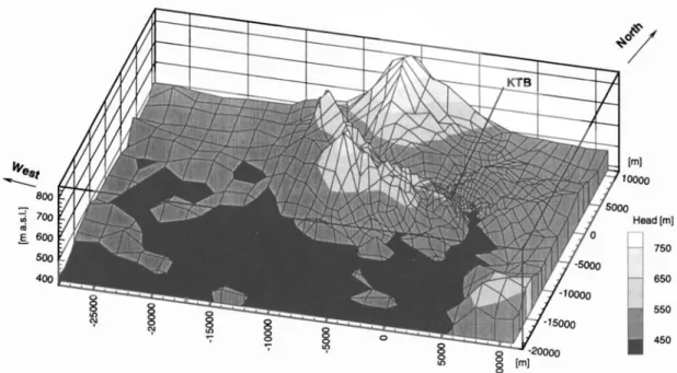
suggest a no-flow boundary for the topography-driven, regional flow field at a depth of 3500 m. The same boundary conditions were taken for all lateral boundaries. Thus, this model assumes no topography-driven fluid flow below the 3500 m depth boundary and a negligible influence of the lateral boundaries at a minimum distance of 10 km on the head distribution near the KTB. The lateral discretization took into account the topographic structures like valleys and mountains, as well as the permeability change between crystalline and sedimentary units. The model was discretized into 9000 nodes and 8900 prism elements with quadrilateral or triangular cross-sections and linear shape functions. Fig. 3 shows the mesh in perspective view.

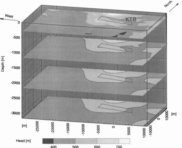
The results of a series of runs performed with a representative model differentiating between crystalline units of low permeability ( m’) and permeable ( m’) sedimentary units are given in Fig. 4, which shows the variation of the

hydraulic field with depth. Close to the surface a rather dispersed flow pattern can be recognized. This tends towards a N-S directed flow at greater depth. The differences in the head distribution decrease with depth, resulting in the strongest flows in the near-surface layers. The mountains of the southern Fichtelgebirge and the lows of the southern valleys dominate the hydraulic behaviour. The flow field at the Frankonian Lineament, which represents an impressive, easily visible surface structure and separates the sedimentary units in the west from the crystalline block, is not connected to the KTB site. This contrasts with the 2-D models of Clauser & Huenges (1993) and Jobmann & Clauser (1994). The local flow field in the vicinity of the KTB is mostly influenced by the nearby valley of the Fichtelnaab River.

A reduction of the lateral block size of this regional model

to create a more detailed local model can only be made if there are no significant horizontal components of hydraulic flow at the lateral boundaries of the smaller model. The definition of such a Neumann-type boundary condition for the hydraulic field can only be performed on ridges or on deep

Figure 3. Finite-element discretization, elevation and surface head distribution of the 3-D regional model. The mesh follows the topographical units and is most refined in the vicinity of the KTB (at 0, 0, 505).

(7)

762

T.

Kohl and L. Rybach

Figure 4. 3-D regional hydraulic situation. The tetragons indicate the boundaries of the smaller block extracted for the local model. Note that the KTB is not located in the centre of the small block.

valleys. Fortunately, a central zone was found (indicated by the tetragon in Fig. 4) that fulfils this requirement. This zone is bounded by the Fichtelnaab River in the north and the Waldnaab River in the east, by the nearly 700 m high altitudes in the west and SW (Kiihberg) and by the NE-dipping slope

of the hills south of the KTB. In contrast to the hydraulic flow field with its dominantly horizontal components, the thermal heat-flow field is directed nearly vertically upwards. Thus, the model with a nearest boundary at 2 km distance from the KTB-VB does not influence the thermal field at the VB.

Due to the topographic constraints the local model's shape is not rectangular. The model extends in an E-W direction over 10 km, and in a N-S direction from 3 km at the eastern border to 7 km at the western border. The northern boundary

is located close to the KTB (about 2 km away).

The advantage of a smaller block model is obvious: due to computer storage restrictions the large regional model could not be discretized finely enough. The small model, however, uses elements with a length of 50 m in the vicinity of the KTB. Thus, structural constraints from surface or borehole geology (fracture zones, small lithological heterogeneities) could be taken into account. At larger lateral distances the mesh becomes coarser, with lateral element lengths up to 500 m. The total domain contains four different geological units: Cretaceous sediments in the west, granite in the NE and gneiss and metabasite in the central region. A perspective view of

this model is displayed in Fig. 5. The final model contained 8000 linear elements with a total of 9000 nodes.

The following procedure was chosen for assigning the material distribution to the model. The large-scale surface geology, like metabasite, (steep) gneiss and granite, was pro- jected into the subsurface. A fit of the measured data set required a variation of the geological units with depth, with the exception of the granitic intrusion. The properties of the metabasic and gneissic blocks were allowed to vary with depth. The depth of that small part of the large granitic intrusion NE of the KTB which falls within the model geometry was taken to be 2000m, in agreement with the Hirschmann (1993) interpretation. The only depth information available is represented by the KTB-VB profile. The KTB-VB site is defined by a vertical column with a 100 m x 100 m cross-section that contains the measured borehole profile. The material properties of this column, which correspond to the measured data set, remained unchanged during the modelling process. Furthermore, the steeply dipping, 400 m wide Nottersdorf Fault Zone (Hirschmann 1992; see also Fig. 6) was investigated especially carefully, since it likely represents an important tectonic unit for the uppermost temperature field. An enlarge- ment of the surface material distribution in the vicinity of the KTB-VB that contains these five units (gneiss, metabasite, granite, the KTB-VB site and the Nottersdorf Fault Zone) is shown in Fig. 6.

The next section describes a thermal diffusive simulation of this second model. Based on varying permeability assumptions, a refined hydraulic field will be evaluated and quantified for its thermal implications in a later step.

(8)

Thermal and hydraulic aspects of K T B 763

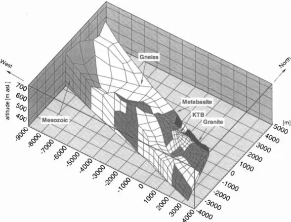
Figure 5. Perspectivic view of the local 3-D thermo-hydraulic model. The figure represents topographic heights, geological units and discretization between the surface and 350 ni. In the x-y plane, the Kuhberg is located near the coordinates (-7000,O).

A

0

3

Figure 6. Geological structures in a block with 1 km2 horizontal cross-section around the KTB. At the surface, the domains 1 and 3 correlate to gneiss, domain 2 to metabasite and domain 4 to granite. Domain 3 represents the Nottersdorf Fault Zone. KTB represents the

VB location.

5.3 3-D thermal model

First efforts at thermal modelling concentrated on describing the measured temperature profile by purely diffusive assump-

tions. Since the foliation of the gneissic and metabasic structures is very steep, abrupt lateral changes of the adjacent material are likely. Locally, at the KTB site, material changes (i.e. changes from gneissic to metabasic structures) were allowed for each of the three adjacent domains (the granitic intrusion remained fixed), as illustrated in Fig. 6. However, this procedure still imposes strong restrictions on a data fit.

(1) The chosen geometry remained unchanged. Since the central KTB domain has a lateral cross-section of 100 m x 100 m, a lateral effect has to extend over a minimum distance of 50 m.

( 2 ) The only materials to be interchanged laterally were

gneiss and metabasite. Although the fitting process allows for a complex lateral geometry, the simplest distribution model (consisting of the mean gneissic and metabasic properties) in the domains adjacent to the KTB was assumed.

An altitude-dependent surface temperature with a free air gradient of 0.004 K m-l was taken. The extrapolation of the

VB temperature log results in a surface temperature of 8.5 "C,

whereas BHT measurements indicate 7.4 "C at the surface.

Therefore, the ground surface temperature was fixed at the KTB as 8 "C. A measured temperature value was taken as the lower boundary temperature of the model (103 "C at 3500 m). No lateral heat flow was assumed at the lateral boundaries. Thus, the lower boundary is sufficiently far away from the uppermost 2000 m depth section considered here. Since the

VB provided reasonably good temperature logs and excellent

(9)

764 T. Kohl and L. Rybuch

will only be compared to the VB observables. Necessary criteria for the model are a satisfactory fit of the measured temperature and temperature gradient. Since the thermal properties of the KTB remained fixed and were taken from core measurements, a fit of the temperature gradient automatically provides a good heat-flow fit.

The best fit was achieved with model run D03a (Figs 7 and 8). The constraints of this model will be discussed only for a block with a 1 km2 cross-section around the KTB. For the purpose of our overview attempt, this block characterizes best all the 3-D implications of the temperature field. In Fig. 7 the material distribution, the temperature gradient and the heat flow are illustrated for this block. A somewhat extreme prop-

erty distribution had to be chosen to fit the temperature profile. Especially for the thermal conductivity between 200 and 500 m, a model had to be chosen that assumes a small, isolated metabasic body, surrounded by gneissic complexes. The lithology in the 200 m distant HB drillhole, where mostly gneiss was encountered in this depth range, supports this assumption. The model suggests two different sections with a continuous transition in between. The uppermost depth section down to 1200 m is dominated by the gneissic influence. This is substan- tiated by surface geology and the VB profile, where gneiss was encountered between 500 m and 1200 m. Our model predicts about 75 per cent gneissic material and 25 per cent metabasite in this section. This is in good agreement with the material

Diffusive Model D03a

Therm.Conducitvity RedTemperature

distribution known from the surface that shows 65 per cent gneissic or granitic and only 35 per cent metabasitic material. The second depth section between 1200m and 2500m is mainly dominated by metabasite. In the vicinity of the KTB, the best-fitting model requires about 80 per cent metabasite and only 20 per cent gneiss. This material distribution does not reflect, however, the characteristics of the cored material, which consists mainly of gneiss. Such results suggest a 'chimney' effect, with heat preferentially flowing along the well- conducting, small-volume gneissic rock masses. A predomi-

nantly metabasic portion of the surrounding rock masses can explain the high-vertical-gradient zones that were measured in the gneissic part of the VB profile at about 2000 m depth.

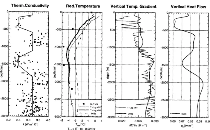
Fig. 8 compares the three measured VB observables of thermal conductivity (vertical component), temperature, and vertical temperature gradient (averaged over the approximate mesh size of 100mf to a 1-D profife extracted from model D03a. With the exception of the uppermost 200m, a good data fit was achieved. The characteristic decrease in the reduced temperature representation (on the basis of a mean gradient of 0.028 K m-') cannot be completely simulated: a maximum deviation of 1 "C still remains between the logs and the model. The same applies to the vertical temperature gradient, where deviations of 0.002 K m-' are apparent. The undulations of the temperature gradient with the strongest variation in the uppermost 200m (of the order of 0.007Km-') cannot be

2.0 2.5 3.0 3.5 4.0 -5 -4 -3 -2 -1 0 1

h [W m-' K'] ,T, ["Cl

Tm = (T

-

8)

-

0.028*z

Vertical Temp. Gradient Vertical Heat Flow

0.020 0.025 0.030 0.06 0.07 0.08 0.09 0.10

a n az [K m '1 q, [w m-7

Figure 8. 1-D profiles showing the geothermal situation along the KTB-VB profile. The plot on the left-hand side shows the thermal conductivity distribution (dots represent the vertical component of VB core measurements and the straight line represents model D03a). The graph to the right (reduced temperature) shows the two measured temperature logs in the VB as well as the result of model D03a (thick dashed line). The third graph compares the measured and the modelled (thick line) temperature gradients. Finally, the graph on the right-hand side shows the apparent vertical heat-flow profile in the VB borehole.

(10)

MODEL

D03:

PARAMETERS

AND

THERMAL

FIELD

AROUND

KTB

Figure 7. Block diagrams showing the thermal input parameters and the calculated thermal field in the vicinity of KTB for the purely diffusive model D03a. The left-hand diagram shows the distribution of gneiss, metabasite and granite (to the very North East). The illustration in the centre shows the vertical temperature gradient distribution, and the right-hand illustration shows the corresponding effects on the vertical heat flow.

(11)

(12)

Thermal and hydraulic aspects

of

K T B 765

simulated by this model. Unfortunately, the uppermost 200 m are not very well documented by the field measurements and thcrefore do not constrain model D03a well (only three thermal conductivity measurements down to 200 m are available; see also Bucker et al. 1990). For an explanation of this feature

further heat-flow mechanisms can be considered. Due to the abrupt changes, these small-sized effects seem to indicate advective thermal transport rather than palaeoclimatic influence.

In summarizing these results, we see that a 3-D thermal diffusive model is able to explain the presence of a low-heat- flow zone in the upper 500 m, as described in Section 2. The onsatisfactory fit of the uppermost 200 m may be improved by assuming advective thermal transport.

5.4 3-D local hydraulic model

The influence of advective heat transport on the temperature field can only be assessed by using geometrically simple models. It is clear that such basic models will not represent perfectly the hydraulic behaviour in the crystalline subsurface. High permeability zones will show up as rather distinct hydraulic effects on the thermal field. Lack of data for a sophisticated hydraulic simulation has lead to the investigation of three alternative hydrogeological assumptions.

( 1 ) 3500 m (deep) homogeneous permeability (run

‘d’).

Table 2. Description and parameters of hydraulic models. Description High permeable structure Run ‘d’ Homogeneous 2 x 10-15 m2

General hydraulic behaviour is highlighted by a flow circulation down to a depth of 3500 m.

(2) 500 m (shallow) homogeneous permeability (run ‘e’). This model characterizes shallow flow circulation, limited to a depth of 500 m.

(3) Nottersdorf Fault assumption (run ‘f’). This model contains the hydraulically most active structure with an assumed model depth of 800 m.

These three models are summarized in Table 2. The effects of the three assumptions on the thermal model D03a are then needed, together with the measured temperature data, to evaluate a realistic permeability distribution.

The calculations performed on homogeneous model (run ‘8)

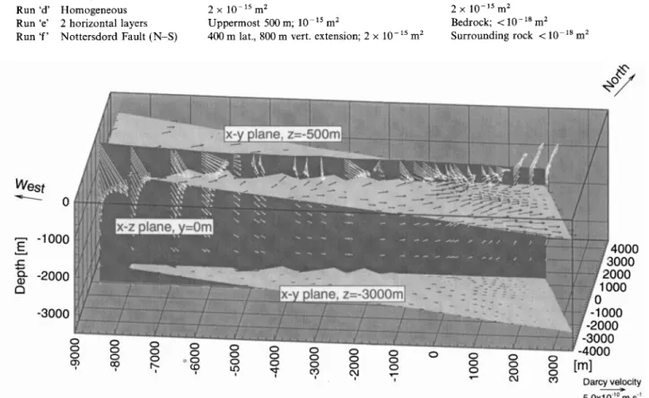
will be described in more detail, because they illustrate very clearly the hydraulic impact. Astonishing effects are revealed. The SW-NE flow in this model has a direction nearly opposite to the overall regional trend (from north to south). From 200 m downwards, rising fluids are expected near the vertical KTB profile. In the fence diagram of Fig. 9 the pattern of downwards fluid migration due to the presence of the hills in the west (Fig. 5 ) can be recognized. The local hydraulic low, which is represented by the Fichtelnaab Valley (Fig. l), is of rather small dimension (width 100-200 m). Therefore, the deeper fluids start rising before reaching the KTB site, whereas the near-surface fluids are still percolating downwards. For a given permeability of 2 x m2 the equilibruim between

Low permeable structure 2 x 1O-l’ mz

Run ‘e’ 2 horizontal layers Uppermost 500 m; mz Bedrock; <lo-’* mz Run ‘f’ Nottersdord Fault (N-S) 400 m lat., 800 m vert. extension; 2 x m2 Surrounding rock i lo-’* mz

Figure 9. The local hydraulic flow field for a hypothetical uniform permeability of m2. The KTB is located at x / y = O/O. The vertical flow field in the east-west direction through the KTB (i.e. the x-z plane) is indicated by white arrows; the horizontal flow field at depths z = -500 m and z = -3000m (i.e. x - y planes) is indicated by black arrows. The flow field at the KTB below 200m is upwards- and above 200m downwards-directed.

(13)

766 T. Kohl

and

L. Rybach -500 -1000 -1 500 E

s

-

Y Q a -0 -2000 -2500 -3000-

downward- and upward-percolating fluids at the KTB location is attained at a depth of about 200 m.

High permeabilities are required to create a sensible thermal effect. Only permeabilities greater than m2 show a clear, characteristic hydraulic impact on the thermal field. This high value is necessary to allow sufficient fluid flow under the driving influence of the low mean head gradient on the surface from the Kuhberg to the Fichtelnaab Valley (-0.03) and due to the rotation of the main drainage axis from the 120"N strike of the Fichtelnaab to the 180"N strike of the Waldnaab. This directional change causes a convex, diverging flow pattern and thereby tends to reduce the flow intensity.

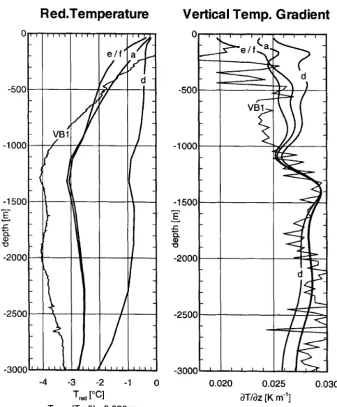
The implications for temperature and temperature gradient of all three models are shown quantitatively in Fig. 10. A

uniform permeability of 2 x lo-'' m2 for the 3500 m deep model was chosen, which is one order of magnitude greater than the highest measured permeabilities. Upward fluid motion at greater depths will cause a heating of the subsurface below the KTB location. Since a Neumann-type hydraulic boundary condition and a fixed temperature boundary condition were applied at

0 7 /

-

Red.Temperature

-4 -3 -2 -1 0 T, ,

["CI

T,, = (T

-

8)

-

0.028*~

the base of the model, the rising fluids yield a maximum deviation of the temperature from the diffusive model at 1200 m

(- 1/3 of the model depth). Models that assume boundaries deeper than 3500 m will show similar effects: the temperature difference between the thermo-hydraulic and the purely diffusive models will increase to a maximum at a characteristic depth and decrease thereafter. Thus, from a thermal point of view, deep circulation/high permeability flow models for the KTB site can be discarded, since the upward-directed flow pattern would lead to lower gradients at greater depth ranges and higher gradients at shallower depths, an effect opposite to the measured thermal profiles.

The second alternative model assumes a shallower flow down to 500m depth and leads to a different thermal effect.

Infiltrating from the cool surface, the fluids percolate downwards in the subsurface. The cooling effect dominates. Model 'e' shows the thermal impacts for this shallow model, which assumes a uniform permeability of m2 for the uppermost 500m and 10-"m2 for the region below. It is obvious that only the uppermost depth range is affected by the circulation.

Vertical Temp. Gradient

0.020 0.025 0.030

avaz

[K m"]

Figure 10. 1-D profiles showing the influence on reduced temperature and temperature gradient of two different hydraulic models. Model run 'd' represents the result of a homogeneous permeability distribution, run 'e' represents the result of a homogeneous permeability at shallow depth, and run 'f' represents the Nottersdorf-Fault case. The curves of runs 'e' and 'f' are nearly identical. Additionally, the diffusive model D03a ('a') and the first VB temperature log ('VBl') are plotted.

(14)

Thermal and hydraulic aspects of K T B 767 A further sophistication of this approach is potentially able to

explain the low-temperature gradient in this upper section. However, another approach seems indispensable, since the hydraulically active fractures in the uppermost 800 m section of the VB can all be related to the Nottersdorf Fault Zone (Hirschmann 1992). The 400 m broad, 160"N striking and 60" to 90" eastward-dipping Nottersdorf Fault Zone is situated close to the KTB. The outcrops of this fault zone range from 560 m down to 440 m elevation at the Fichtelnaab River. The neighbourhood of the Nottersdorf Fault Zone down to 800 m depth is likely to be characterized by higher permeability than the surrounding materials. Thus, it may strongly influence the flow field near the KTB.

An effective thermal transport by the Nottersdorf Fault model (run 'f') requires high permeabilities. These are due to the even smaller head gradient on the surface (0.02), since the 160" striking profile of the fault zone is not oriented parallel to the steepest surface inclination. For model 'f' a permeability of 2 x m2 for the Nottersdorf Fault down to 800 m depth and 10-18m2 for the surrounding rock masses is assumed. Like run 'e' this model yields a strong decrease of the thermal gradient in the upper 150m. The temperature field in the deeper section, which is well represented by the diffusive model D03a (run 'a' in Fig. lo), is only slightly affected.

It is evident that 3-D considerations are indispensable for the evaluation of the local hydraulic flow regime, since the meso-scale variations of topographic height around the KTB site cause a complex flow pattern in the subsurface. A 3-D flow analysis reveals only rarely a planar 2-D flow but more often a convex, diverging (like at the KTB site) or concave, converging flow pattern. Models that contain a rather complex thermal conductivity distribution and assumptions on permeabilities which restrict hydraulic flow to shallow depth are well suited to describe the measured temperature profile in the upper 200m of the KTB site. The hydraulic considerations are confirmed by Jobmann (1990) and Stiefel(l990) who have detected hydraulically active fracture zones in the upper part of the VB that are located at 300 m, 500 m and 600 m depth. A topographically driven hydraulic flow field can only be inferred for the uppermost section of the drilled depth. Our considerations strongly suggest purely diffusive thermal transport for the main part of the drilled KTB depth range. A different model assumption led Jobmann & Clauser (1994) to a similar conclusion. For various reasons drill sites are often situated on high ground. The KTB site follows this pattern. In a terrain with high permeability at shallow depth, a drill hole at such sites is likely to be exposed to downward-percolating fluids. This mechanism could be responsible for the erroneous temperature prediction during the site investigation study (see, for example, the location of drillholes Pullersreuth and Rummelsberg on Fig. 1; cf. Burkhardt et al. 1989).

6 T H E R M A L S I M U L A T I O N O F D R I L L E D KTB-HB D E P T H

6.1 Geological cross-section

This second simulation was aimed at the investigation of thermal effects along the drilled depth of the KTB-HB, i.e. the upper crust. It was intended to set up a thermal model for the KTB location containing the available geological knowledge and accounting for realistic heat-flow mechanisms. As shown

above, no thermally significant fluid flow can be expected over most of the drilled depth.

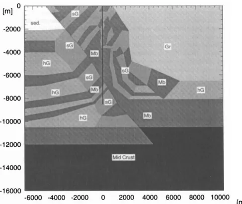
The most complete geological interpretation for the drilled KTB section is presented by Hirschmann (1993). It is based on direct borehole data, on geological mapping and on geo- physical surveys in the KTB region. He describes a SW-NE striking profile with strongly dipping gneissic and metabasic structures at the ZEV. The region is bounded laterally by surface sediments to the SW and by granitic intrusions to the NE. The chosen SW-NE profile direction is parallel to the strike of the gneissic structures as observed in the borehole profile. The lack of information along the NW-SE direction (perpendicular to the Hirschmann profile) is obvious; however, surface geology does not indicate any abrupt lithology change in the third dimension. Therefore, a 2-D approach to the greater part of the drilled depth down to 9 km seems to be appropriate. Fig. 11 shows the material distribution in the discretized domain. Clearly, the same features as on the Hirschmann profile are present: 60" dipping alternating lateral gneissic and metabasic formations are situated in the centre of the ZEV near the KTB, and at a lateral distance of 5 km horizontally layered units (near-horizontal gneiss) are encountered. Fig. 11 is slightly different from the Hirschmann profile since the model runs that fit the BHT measurements best require a lateral shift of up to 300m of the surrounding geological units.

Due to its greater depth range, the second model takes mid- crustal material into account as well. The choice of the mid- crustal material is not very critical with respect to thermal conductivity, since its temperature dependence leads to a rather small bandwidth of variation, as discussed above. The thermal properties of the materials used for this 2-D simulation (sediments, near-horizontal gneiss, steeply dipping gneiss, granite, metabasite, mid-crustal material) are summarized in Table 1.

6.2 2-D thermal model

In Fig. 12 the refined finite-element mesh around the KTB is shown. This model consists of 3000 nodes. Different model runs have shown that finer spatial discretization or the use of quadratic elements produces no significantly better results. For practical reasons it was decided to accelerate calculations by using the linear rather than the quadratic elements.

A mean annual surface temperature of 8 "C was assumed as

the upper-boundary condition. The lower boundary was placed at a depth of 16 000 m in the mid-crustal region, deep enough to have no effect at the depth range considered. Since neither the temperature field nor the heat flow is known for that depth, a plane of constant basal heat flow was assumed. The vertical heat flow at the lower boundary was varied in order to fit the measured temperature data. An optimum value of 0.063 W m-2 was found, which corresponds to a temperature of 437 "C at a depth of 16 km below the KTB.

The lateral boundaries are located at a distance of 6 km SW and 10 km NE of the KTB, where a vertical heat-flow field is assumed. The distance is sufficient to leave the temperature field around the central area below the KTB uninfluenced by the boundary conditions. The simulation runs demonstrated that the lateral component of the heat-flow vector is negligible except in the more steeply dipping gneissic zones, where it reaches 10 per cent of the total heat flow.

(15)

768 T. Kohl and L. Rybach

Figure 11. Material distribution of the discretized Hirschmann (1993) profile. The origin of the coordinate system corresponds to the borehole location on the surface. The black line represents the drillhble. Gr = granite, hG = near-horizontal gneiss; sG = steep gneiss; and M b = metabasite.

0 -1000 -2000 -3000 -4000

-

_E 5 -5000 I a -a -6000 -7000 -8000 -9000 -4000 -2000 0 2000 4000 distance from KTB [m]

Figure 12. Detail of the finite-element mesh in the near field around the KTB created by the mesh generator FRAM. The black line represents the drillhole down to a depth of 9000 m.

the model in the VB depth section. The BHT values recorded during the HB phase can give information on the temperature profile at discrete points but cannot be used to evaluate the temperature gradient. This represents the strongest restriction for the final evaluation of the model, since we consider the thermal gradient as the most critical parameter for these steeply dipping zones (see later).

The results of the 2-D model will be discussed for the central ZEV region only; the peripheral regions of the model are

subject to speculation. It must also be pointed out that deviations from the observed heat-flow distribution must be expected for the uppermost 1000 m because it was not intended to optimize the uppermost heat-flow zone using this diffusive model.

Fig. 13 shows the modelled depth distribution of the vertical components of thermal gradient and heat flow. In the vicinity of the KTB, a rather constant gradient accompanied by a stronger heat-flow variation can be recognized. A comparison of the model profile to the available temperature data is given in Fig. 14. In the central part of the Hirschmann (1993) section the thermal behaviour can be described best if the material distribution of Fig. 11 is compared to the thermal gradient field in Fig. 13. A maximum variation of the thermal gradient of the order of 10 per cent can be found that is far lower than the 20 per cent in variation in thermal conductivity. The usual inverse correlation of thermal conductivity with gradient is found only in the horizontally layered materials close to the lateral boundaries. Different hypothetical observation boreholes in the heterogeneous central part of the model would not show a strong change in thermal gradient. This effect suggests that temperature logging performed in a hypothetical adjacent (- 1 km) borehole would not differ strongly from the KTB temperature measurements. The KTB, HB and VB themselves (200 m apart) demonstrate this. The BHT measurements in the HB coincide well with the VB temperature profile (except for the two first BHT values, which are probably inexact because they were measured at a large borehole diameter and were therefore submitted to borehole convection). This fact can be considered as justification of the fixed temperature boundary condition in the 3-D model in Section 5.3.

Thus, the general pattern of a uniform gradient distribution 0 1996 RAS, G J I 124,156-772

(16)

Thermal and hydraulic aspects of

K

T B 769 observed along the entire drilled depth section can be

explained. Apart from the upper 500 m, the observed temperature gradient can be represented well by the model profile (Fig. 14). The strongest deviations occur around 3200 m and 4000 m. The general diffusive character of the thermal transport in the crystalline domain is not thrown into question by these two deviations, because they coincide with fractured zones near large fluid reservoirs (Huenges 1993). The importance of a local temperature perturbation due to these reservoirs can only be explained after further temperature logs are made, since due to their preferential uptake of drilling mud these zones are most affected by the drilling process.

The heat-flow variation in the central domain is stronger than the variation in temperature gradient (Fig. 13 bottom).

As expected, heat flows preferentially along the steeply dipping

gneissic units. Small (500 m) lithology variations in the subsurface result in a strong change. Near the lateral boundaries, the heat flow shows the uniform behaviour expected in horizontally layered materials. The area around the drill hole at about 6 km depth indicates that the lateral extension of such a heat- flow anomaly extends more than 500 m into the metabasite. On the other hand, sensitivity analysis performed on different conductivity values has demonstrated that the borehole profile is completely unaffected by the choice of granitic or of sedimentary material properties. The effect of strongly decreasing heat flow in the granitic area is due to the effect of decreasing thermal conductivity with depth, as well as to the high heat production.

Fig. 14 shows the results of our model along the drilled section, down to a depth of 10 km. Also plotted are the measured observables of thermal conductivity, temperature and vertical temperature gradient (averaged over the approximate mesh size of loom), which are available from cuttings and logs. The deviations between the model and the BHT values are within a bandwidth of 2 K. This must be considered as satisfactory in view of the uncertainties in the data themselves. The BHT values and temperature logs in the VB vary relative to each other by as much as f 2 K. Thus, the data available for the HB do not allow a further refinement of the model at this stage.

7 T H E R M A L E F F E C T S I N DIPPING

LAYERS

It has been demonstrated that the available borehole temperature data and geological inference provide the basis for an unambiguous geothermal interpretation of the upper crust by thermal diffusion at the KTB site. In steeply dipping zones with alternating thermal conductivity distribution, the analysis of the heat flow alone might lead to erroneous results. In ground-water flow analysis this represents a commonly known effect (Freeze & Cherry 1979). By demanding continuity for the flow component normal to the interface, a simple graphical construction of dipping flow lines penetrating into a horizontally layered medium with contrasting thermal conductivities yields a refraction effect. The following 2-D example, calculated with FRACTure, has been chosen to illustrate this effect in the geothermal context.

Assume an infinite, layered underground consisting of two materials with thermal conductivities I , and 1,. Heat flows vertically and uniformly in the subsurface; heat production is ignored. The interface between the two materials is rotated

about the coordinate origin (0,O) to dip between 0" (horizontally layered) and 80" (nearly vertical). A hypothetical vertical borehole penetrates the interface at the point (0,O). Fig. 15 characterizes the temperature gradient and heat-flow profiles that would be encountered in this borehole. For a horizontally layered medium, the general pattern of uniform heat flow across the interface and a discontinuity in the temperature gradient at the interface are found. As the dip angle is successively increased, the temperature gradient tends to become uniform, and the derived heat-flow profile tends to take a discontinuous form. The magnitude of the variation depends linearly on the initial values of 1, and I , (in our calculation I , = 1.51, is assumed) and can therefore be easily derived for different conductivity ratios. A 90" dipping structure results finally in a vertical uniform mean gradient that takes into account the portion of the two adjacent materials.

The KTB seems to offer an excellent demonstration of the influence of lateral heterogeneities. Even under the assumption of a 2-D structure (Fig. 11) the 60" dipping units cause heat- flow perturbations over a long distance ( < 1 km). Therefore the thermal field of Fig. 13 can be explained by applying the results of the example discussed above. In such steeply dipping structures 'apparent vertical heat flow' has been the term suggested. Thus, it becomes evident that in steeply dipping structures it is not possible to apply a conventional interpretation of heat-flow regimes derived from geothermal research in horizontally layered, sedimentary basins or simplified 1-D structures, such as that described by Chapman & Furlong (1992). The apparent heat flow is not easily interpretable since small lateral structural changes result in different heat-flow values and might suggest (erroneously) additional heat-transport mechanisms. In such cases, the interpretation should focus on the temperature gradient. The magnitude of the gradient reflects the proportions of adjacent materials. Ignoring the local conductivity measurements, this simple 2-D model suggests that an inverse analysis can lead to an estimation of a mean thermal conductivity of the adjacent rock for 90" dipping interfaces, if assumptions on the mean heat-flow field are available. The KTB data sets allow an easy comparison of the mean conductivities with the two cored materials, gneiss and metabasite. A first-order estimation (ignoring heat production, assuming two-dimensionality and nearly subvertical structures) that assumes a mean heat flow of 0.075 W rn-' and a temperature gradient between 400 m and 1100 m of 0.024 K m-l yields a surrounding material with a mean thermal conductivity of 3.1 W m-l K-l. This value corresponds to a composition of 89 per cent gneiss and 11 per cent metabasite if the thermal conductivities of Table 1 for steeply dipping gneiss and metabasite are applied. A temperature gradient of 0.028 K m-l measured below 1100 m yields 25 per cent gneiss and 75 per cent metabasite. A comparison with the results of the more sophisticated 3-D thermal model of Section 5.3 shows rather small differences (D03a: 65 per cent/35 per cent and 20 per cent/80 per cent respectively). This demonstrates that a quantitative estimation of the relative portion of the surrounding gneissic and metabasic material is possible even under the conditions of the complex geology at the KTB site.

Similar estimations have been performed by Huenges et al. (1994). By comparing the rock density distribution in the HB derived from borehole gravity data with the distribution of the gneissic and metabasic cuttings, they conclude that the gneissic portion in the upper 6 km outweighs the metabasic portion.

(17)

770 T. Kohl and L. Rybach

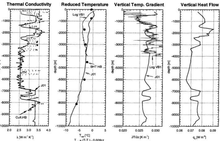
2D Model JOI

Thermal Conductivity Reduced Temperature Vertical Temp. Gradient Vertical Heat Flow

2.0 2.5 3.0 3.5 4.0 -10 -5 0 5 0.020 0.025 0.030 0.06 0.07 0.08 0.09

Figure 14. Comparison of the 2-D model JO1 with the KTB observables. The plot on the left-hand side shows the measured conductivities from the HB cuttings and a vertical conductivity distribution, which is interpolated from the model to the KTB-HB profile. The diagram to the right of this compares the reduced temperature (reduced by a mean gradient of 0.028 K m-’) of the model (run ‘JOl’) with BHT measurements in the HB and with the last VB temperature log. The third graph compares the calculated vertical thermal gradient with the vertical gradient profile of the VB temperature log. The right-hand plot illustrates the apparent vertical heat-flow profile calculated by the model.

: : : 1 -r 300 E 0 -400 -500 -30 -20 -10 0

h,

=

1.5 h,

variation of q [%I variation of aTBz [“YO]

Figure 15. Variation of the vertical components of heat flow q and temperature gradient with dip angle GI of the thermal conductivity interface.