Réaction fonctionnelle des arbres et des
peuplements à l’éclaircie commerciale en
forêt résineuse
Mémoire
Simon Boivin-Dompierre
Maîtrise en sciences forestières
Maître ès sciences (M. Sc.)
Québec, Canada
iii
Résumé
Globalement, on connait bien les objectifs et les effets théoriques de l’éclaircie commerciale. Cependant, peu de résultats expérimentaux sont disponibles au Québec pour confirmer que l’application d’un tel traitement permet d’atteindre les objectifs et de bien répondre aux attentes. Pour pallier à ce manque, nous avons étudié des peuplements traités il y a 7 à 10 ans et localisés dans des forêts résineuses du sud du Québec. Nous avons évalué la réaction des arbres et des peuplements par le biais de variables agissant sur leurs processus de croissance. Pour ce faire, nous sommes retournés dans des placettes échantillons permanentes établies dans les années 1980 et 2000 pour y caractériser la taille des cimes et l'environnement compétitif d’arbres éclaircis et non éclaircis en plus des mesures dendrométriques usuelles. Nous avons aussi prélevé des carottes dendrométriques qui ont permis de reconstituer la surface foliaire des arbres à partir de leur surface d'aubier au moment de la coupe. L’utilisation de modèles linéaires mixtes a permis de démontrer que les accroissements en surface terrière et en surface foliaire des arbres sont fortement liés à leur localisation par rapport au sentier de débardage le plus près. La compétition, quantifiée par un indice indépendant de la distance, a expliqué une proportion importante de la réaction des arbres. Par rapport aux peuplements témoins, l’éclaircie a augmenté la quantité de bois produite par unité de surface foliaire sans toutefois mener à un accroissement supérieur en volume marchand à l’hectare étant donné le plus faible nombre d’arbres. Ces résultats viennent donc éclairer notre compréhension des processus agissant sur la croissance des arbres après un traitement d’éclaircie commerciale. Ils pourront aider à déterminer l’aptitude de peuplements à l’éclaircie et servir à l’élaboration d’outils d’aide à la décision lors du choix des arbres à récolter.
v
Table des matières
Résumé ... iii
Table des matières ... v
Liste des tableaux ... vii
Liste des figures ... ix
Remerciements ... xiii
Avant-propos ... xv
Introduction générale ... 1
Functional response of coniferous trees and stands to commercial thinning in eastern Canada ... 6
Abstract ... 6
Introduction ... 7
Materials and Method ... 10
Study area ... 10 Experimental design ... 10 Data collection... 11 Competition index ... 12 Leaf area ... 14 Growth efficiency ... 15
Modeling growth response to thinning ... 16
Statistical analysis ... 17 Results ... 18 Tree scale ... 18 Stand scale ... 23 Discussion ... 26 Spatial effects ... 26 Non-spatial effects ... 27 Silvicultural implications ... 29 Conclusion ... 31 Conclusion générale ... 32 Bibliographie ... 34
vii
Liste des tableaux
Table 1 Competition indices compared in this study ... 12 Table 2 Mean stand characteristics of control and thinned plots before, after and seven to ten years after thinning ... 18 Table 3 Coefficient values for Eq. 13 ... 20 Table 4 Statistics of competition index models fitted according to Eq. 3 ... 22
ix
Liste des figures
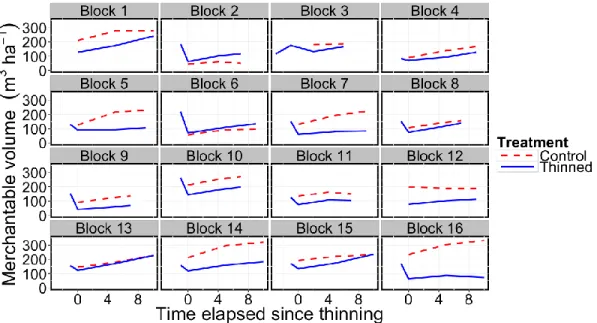
Figure 1 Hypothèses de productivité de l’éclaircie commerciale ... 2 Figure 2 Tree basal area increment (BAI) as a function of distance from the nearest skidding trail. ... 19 Figure 3 Temporal changes of tree leaf area (A) and growth efficiency (B) in control plots and for two distance classes from the nearest skidding trail in thinned plot .... 21 Figure 4 Predicted tree basal area increment as a function of the competition index DI4, thinning for balsam fir trees. ... 23 Figure 5 Growth efficiency as a function of basal area in 2014 for thinned and unthinned stands. ... 24 Figure 6 Temporal changes in merchantable stand volume for each pair of plots .. 25
xi
“You can learn a lot by just looking”
-Yogi Berra
xiii
Remerciements
Je tiens d’abord à remercier mon équipe de direction de m’avoir recruté et accompagné au cours de ma maîtrise. Grâce à son incroyable esprit d’analyse, David Pothier, mon directeur, a grandement contribué à la réussite du projet. Son humour unique est aussi digne de mention. Le support d’Alexis Achim, mon codirecteur, a lui aussi été plus que bienvenu notamment par ses grandes capacités de communicateur, motivateur et de chercheur. Je vous remercie de m’avoir fait confiance et pour votre présence.
Je dois aussi remercier Domtar, non seulement pour le financement du projet, mais pour m’avoir donné un accès privilégié aux terrains, bases de données et aux ressources de la compagnie. Merci à Patrick Cartier qui a bien su m’encadrer et m’éclairer sur la réalité industrielle. Un merci spécial à Pierre Duval et Bernard Lapointe que j’ai eu la chance de côtoyer plus régulièrement. Je suis bien heureux d’avoir pu bénéficier de leur expérience et de leur connaissance surprenante du territoire.
Je ne peux passer sous silence l’apport essentiel de Philippe Leduc, mon assistant sur le terrain et plus encore. Je suis bien chanceux d’avoir pu compter sur une aide aussi fiable, travaillante et surtout de bonne compagnie. Merci également à Guillaume Brown, Félix Faucher et Mathieu Bouchard pour leur contribution aux inventaires.
Je salue aussi mes potes du laboratoire de sylviculture : Laurence, Célia, Olivier, Pierre-Yves et Louis-Philippe. Même avec pas de fenêtre, la vie au 2118 était loin d’être triste en votre compagnie.
Merci à ma famille, mes amis et à tous ceux qui se sont intéressés et ont contribué de près ou de loin au projet. Finalement, je remercie le Conseil de recherches en sciences naturelles et génie ainsi que le Fonds de recherche nature et technologie qui ont financé le projet par le biais du programme de bourse BMP - Innovation.
xv
Avant-propos
Je suis l’auteur principal de l’article inséré. Celui-ci est publié dans le journal Forest Ecology and Management. J’ai élaboré le protocole de recherche à l’aide de mon directeur David Pothier. Les données qui ont servi aux analyses proviennent en partie d’un inventaire que j’ai moi-même effectué ainsi que de la base de données de la compagnie Domtar. J’ai réalisé les analyses statistiques, interprété les résultats et rédigé le manuscrit.
Mon directeur de recherche, David Pothier, a participé à l’élaboration du protocole de recherche. Il a fourni d’indispensables avis tout au long du projet sur la méthodologie et l’analyse des résultats. Il a corrigé et commenté le manuscrit ainsi que les documents préliminaires tout au long de leur rédaction. Mon codirecteur, Alexis Achim, a été d’une grande aide pour les analyses statistiques. Il a aussi contribué par ses corrections et commentaires sur l’interprétation des résultats et sur le manuscrit.
1
Introduction générale
L’actuelle mise en œuvre de l'aménagement écosystémique au Québec encourage le recours à diverses coupes partielles en forêts résineuses. Ces traitements sylvicoles sont associés à une large gamme de prélèvement et de structure des peuplements résiduels, ce qui rend difficile la prévision de leurs rendements. Cette problématique est d’autant plus présente dans les conditions tempérées du sud du Québec où les peuplements résineux sont moins abondants et moins étudiés.
L’éclaircie commerciale (EC) fait partie des traitements émulant les perturbations légères à intermédiaires telles que les épidémies d’insecte, les chablis partiels ou le processus d’autoéclaircie qui modifient la dynamique des forêts résineuses (Bergeron et al., 1999). Ce procédé vise à améliorer la valeur individuelle des arbres en redistribuant le potentiel de croissance de la station sur un nombre réduit d’individus. Ainsi, un peuplement non traité devrait produire le même volume à la fin de sa révolution qu’un peuplement éclairci pour lequel on tient compte du volume récolté lors de l’éclaircie et de la coupe finale (Nyland, 2002). L’EC peut aussi être prescrite afin de récolter un volume dans un peuplement prémature pour pallier aux difficultés d’approvisionnement lors de la période critique des calculs de possibilité ligneuse ou pour devancer une entrée d’argent par rapport à un régime ne prévoyant qu’une coupe totale. L’EC est aussi un moyen de récolter les arbres de faible vigueur qui seraient morts avant la prochaine intervention, ce qui évite une perte de volume associée à la mortalité (Nyland, 2002).
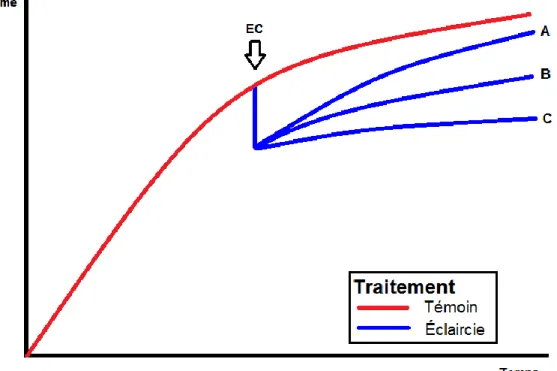
Même si globalement, on connait bien les objectifs et les effets théoriques de l’éclaircie commerciale, trois hypothèses de productivité des peuplements éclaircis comparés à des peuplements non traités sont présentes dans la littérature : 1) des trajectoires temporelles de volume qui convergent, ce qui indique une stimulation de la production de bois par l’EC (Fig. 1A); 2) des trajectoires temporelles de volume parallèles impliquant une redistribution du potentiel de croissance de la station parmi les arbres résiduels (Fig. 1B); et 3) des trajectoires temporelles de volume qui divergent à cause d’une densité résiduelle trop faible ou de la création de grandes trouées qui résultent en une diminution de la production de bois avec le temps (Fig. 1C) (Zeide, 2001; Pelletier & Pitt, 2008).
2
Figure 1 Hypothèses de productivité de l’éclaircie commerciale
Le second scénario est celui qui est habituellement observé et qui fait l’objet du plus grand consensus (Zeide, 2001; Mäkinen & Isomäki, 2004; Pelletier & Pitt, 2008). Cependant, certaines études ont observé des réactions convergentes (Marshall & Curtis, 2002; Soucy et al., 2012; Barrette & Tremblay, 2015) et des réactions divergentes (Loftus, 1996) dans des peuplements résineux éclaircis. Cette variabilité de réaction peut être due à des différences d’âge, de qualité de station, d’intensité de prélèvement, de patron de récolte, d’essences, de structure du peuplement, du type d’éclaircie pratiqué, etc. La provenance de données issues de dispositifs expérimentaux contrôlés ou d’un contexte industriel peut aussi influencer les conclusions (Benjamin et al., 2013; Guay-Picard et al., 2015).
Les trajectoires convergentes sont habituellement associées à de faibles prélèvements répétés selon de courts intervalles de temps. Elles sont donc rarement observées dans un contexte opérationnel puisque les éclaircies sont généralement mécanisées, ce qui nécessite des prélèvements considérables pour assurer leur rentabilité. Ces contraintes mènent à la formation de trouées trop grandes pour
3 assurer l’utilisation maximale de la station et introduisent une hétérogénéité spatiale de la distribution des arbres. Il s’ensuit donc une variabilité de la capacité des arbres à acquérir les ressources disponibles, ce qui active les processus de compétition (Binkley et al., 2004). L’EC brise l’équilibre entre la quantité de ressources disponibles et les besoins des arbres sur pied (Perry, 1985; Jack & Long, 1996). Comme la croissance des arbres est le résultat de multiples interactions entre la disponibilité et l’acquisition des ressources, l’efficacité à les transformer et l’allocation des produits transformés aux différentes parties des arbres (Binkley et al., 2004), les variables décrivant ces processus sont tout indiquées pour évaluer l’effet d’une éclaircie. De plus, ces variables permettent d’identifier des patrons de croissance qui s’appliquent habituellement à différents types de forêt (Oliver & Larson, 1996).
La croissance des arbres est fortement influencée par la compétition pour les ressources, qui peut être manipulée par l’éclaircie. La compétition est habituellement quantifiée au moyen d’indices qui sont ensuite introduits dans des modèles de croissance pour ainsi décrire la variabilité de l’accroissement et de la mortalité des arbres. Leur pouvoir prédictif est variable et dépend de la composition des peuplements étudiés. Deux grandes familles sont habituellement reconnues. Ainsi, on distingue les indices indépendants des distances des indices dépendants des distances, ces derniers nécessitant la localisation exacte de chaque arbre dans la placette. Les premiers se calculent plutôt avec les données usuelles d’inventaire et produisent des résultats généralement adéquats (Prévosto, 2005). Par contre, lorsque les arbres ont une distribution spatiale hétérogène, les indices dépendants de la distance peuvent devenir avantageux (Contreras et al., 2011). Cependant, l’acquisition des données de localisation des arbres est couteuse en temps et en argent, surtout que la supériorité de ces indices n’a pas toujours été clairement démontrée (Biging & Dobbertin, 1995; Roberts & Harrington, 2008; Contreras et al., 2011; Bosela et al., 2015). Toutefois, peu de travaux ont été menés sur la capacité des différents indices à prédire la croissance d’arbres dans un contexte d’hétérogénéité spatiale induite par une coupe partielle (Puettmann et al., 2009; Comfort et al., 2010). Cette hétérogénéité, principalement attribuable à la présence de sentiers de débardage pourrait favoriser la croissance des arbres adjacents (Roberts & Harrington, 2008; Genet & Pothier, 2013)
4
La diminution de la compétition, observable notamment par la création de trouées dans la canopée, implique aussi la réduction de l’indice de surface foliaire (ISF) à l’échelle du peuplement (Jack & Long, 1996). Cette variable est primordiale dans l’étude des processus de croissance puisqu’elle est fortement liée à la transpiration et la respiration de la canopée, et, par conséquent, à la capacité photosynthétique (Vose & Allen, 1988). En effet, la surface foliaire est le reflet de la capacité des arbres à faire de la photosynthèse et est un facteur clé de la réaction de croissance des arbres à une éclaircie (Brix, 1983; Binkley & Reid, 1984; Perry, 1985). Une diminution de la productivité du peuplement devrait ainsi être attendue à la suite d’une EC, mais elle peut être compensée à court terme par une augmentation de la production de bois par unité de surface foliaire, i.e. l’efficacité de croissance (GE – growth efficiency) (Waring, 1983). Ce phénomène est possible car la diminution de la compétition permet aux arbres d’allouer plus de ressources à la production de bois qu’aux organes responsables de l’acquisition des ressources (Brix, 1983; Oren et al., 1987; Velazquez-Martinez et al., 1992). En plus de démontrer l’effet de traitements sylvicoles, l’efficacité de croissance permet d’estimer la vigueur des peuplements (Waring, 1983). À moyen terme, la réduction de l’ISF sera progressivement compensée par la production de feuillage des arbres éclaircis qui combleront les trouées dans la canopée. Le rétablissement de l’ISF initial signifierait que le peuplement a atteint une utilisation équivalente des ressources de la station et devrait mener à des trajectoires de volume parallèles.
L’atteinte d’un scénario à trajectoires parallèles dépend ainsi de l’augmentation de l’efficacité de croissance et de la vitesse de croissance en surface foliaire des arbres dans les années suivant l’EC. Si ces processus ne sont pas effectifs ou si les trouées sont trop grosses pour être comblées par l’expansion des arbres résiduels, il serait plus justifié de s’attendre à des trajectoires divergentes des courbes de production des peuplements éclaircis et témoins (Fig. 1C).
La prescription de traitements sylvicoles adaptés au peuplement tout en étant rentables nécessite une maitrise des effets de tels traitements sur la croissance des arbres. Plusieurs études ont quantifié l’effet de coupes partielles en termes de gains en volume ou de qualité des tiges. Cependant, il semble tout aussi important d’étudier la source de ces effets, c’est-à-dire de comprendre les processus impliqués dans la
5 réaction des peuplements aux interventions sylvicoles. De cette façon, nous serons plus à même de moduler les prescriptions en fonction de chaque peuplement afin d’en améliorer la qualité et la vigueur générale.
L’objectif principal du projet est de déterminer la réaction des arbres et des peuplements aux traitements d’éclaircie à l’aide de relations fonctionnelles faisant notamment intervenir l’environnement compétitif des arbres. Ainsi, le projet déterminera les impacts de l’éclaircie sur la croissance en surface terrière et en volume d’arbres et de peuplements éclaircis. L’hypothèse principale est que la réaction des arbres sera d’abord expliquée par une plus grande production de bois par unité de surface foliaire qui sera suivie, à moyen terme, par une augmentation de la surface foliaire. La seconde hypothèse prévoit que la croissance des arbres augmentera avec une diminution de la distance par rapport aux sentiers de débardage. Nous posons finalement l’hypothèse qu’en fonction de l’augmentation de la taille des trouées due à l’intensité du prélèvement ou à l’occupation des sentiers, on observera un gradient de trajectoires temporelles de volume passant de la convergence à la divergence. Les résultats permettront d’émettre des recommandations afin d’améliorer l’application du traitement de façon à maximiser les rendements et guider les aménagistes forestiers dans leurs choix sylvicoles.
6
Functional response of coniferous trees and
stands to commercial thinning in eastern
Canada
Abstract
The overall objectives of commercial thinning are to increase individual stem growth and, arguably, to increase stand yield. Yet few empirical results are available that would confirm the treatment meets such expectations in an industrial context. We studied the response of stands to commercial thinning with a particular focus on variables that were related to processes of stemwood production at the tree and stand levels. We inventoried permanent sample plots established between 1980 and 2000 in naturally regenerated conifer stands of southern Quebec seven to ten years after thinning. We reconstituted tree leaf area and wood production per unit leaf area using field and dendrochronological data for different years following thinning. Mixed linear models showed that tree basal area and leaf area increments following treatment were strongly related to the tree distance from the nearest skid trail. Wood production per unit leaf area was significantly higher for trees located within 5 m of a skid trail compared to control trees as soon as one year following thinning application, while significant differences in tree leaf area required five years. Compared to control stands, thinned stands had higher wood production per unit leaf area, but merchantable volume increment did not differ. These results provided insight into growth processes that are involved in tree responses to mechanized thinning and could aid in the development of decision tools that determine the suitability of stands for receiving the treatment.
7
Introduction
Commercial thinning (CT) is a type of partial cut that is applied to dense premature stands to increase the diameter growth, quality and vigour of residual trees (Nyland, 2002). There are three hypothetical productivity outcomes for thinned stands compared to unthinned stands: 1) a convergent volume trajectory over time, which implies that CT can stimulate wood production per hectare; 2) a parallel volume trajectory, implying that thinning only redistributes the growth potential of the site among residual trees; and 3) a divergent volume trajectory that is indicative of underutilized growth potential of the site after thinning. The last outcome may be incurred by insufficient stand densities or caused by the presence of large gaps that decrease wood production over time (Zeide, 2001; Pelletier and Pitt, 2008). In all cases, the stand volume trajectory is the net result of survivor growth, ingrowth and mortality (Beer, 1962) but since CT is applied to premature stands, the survivor growth is usually the most important of these three components.
Even if parallel volume trajectories are generally obtained from CT that has been applied in conifer stands (Zeide, 2001; Mäkinen and Isomäki, 2004; Pelletier and Pitt, 2008), some studies have reported both convergent (Marshall and Curtis, 2002; Soucy et al., 2012; Barrette and Tremblay, 2015) and divergent (Loftus, 1997) responses. These conflicting results may be associated with differences in thinning types (e.g., low vs high thinning), application methods (e.g., mechanized vs manual), site conditions, or tree species. While controlled experiment designs are useful, they do not generally include the many constraints and sources of variability that are associated with large-scale operational treatments (Benjamin et al., 2013; Guay-Picard et al., 2015). From an operational perspective, thinning must remove a sufficient volume of merchantable wood to generate profits, which in turn may prevent the volume growth trajectory of the thinned stand from converging on that of an unthinned stand. Indeed, gaps that are created by the passage of harvesting machinery may limit resource acquisition to a suboptimal level at the stand scale by introducing spatial heterogeneity in tree distribution and competition (Perry, 1985; Jack and Long, 1996; Binkley et al., 2004).
8
Inter-tree competition is usually quantified by various indices, which have been tested through empirical studies under several conditions where they reasonably describe the interactions between a tree and its environment (Contreras et al., 2011). These indices can be classified as distance-dependent or distance-independent. Distance-dependent indices take into account the distances between trees and are used to represent the spatial heterogeneity of a stand (Contreras et al., 2011). Acquiring tree spatial locations is time-consuming and costly, and the superiority of distance-dependent indices in predicting stemwood growth has yet to be clearly demonstrated (Biging and Dobbertin, 1995; Roberts and Harrington, 2008; Contreras et al., 2011; Bosela et al., 2015). Distance-independent indices are simpler and usually can be computed from forest inventory data. Yet little is known regarding the abilities of the two types of indices to predict tree growth in the context of spatial heterogeneity that is caused by partial cutting (Puettmann et al., 2009; Comfort et al., 2010). This heterogeneity, which is mainly due to the presence of skid trails, could stimulate the growth of only certain trees, thereby creating pronounced spatial patterns of response to thinning (Roberts and Harrington, 2008; Genet and Pothier, 2013).
One limitation of the relationships between tree growth and competition indices is that they are only applicable to the conditions under which they have been calibrated. In order to generalize tree growth patterns in relation to their competitive environment, it is necessary to take into account the complex interrelationships between resource availability and acquisition, resource use efficiency, and biomass partitioning between tree parts (Binkley et al., 2004). Indeed, focusing upon the fundamental drivers of stem growth can help predict response patterns that are applicable to a wide range of stand conditions and forest types (Binkley and Reid, 1984). At the stand level, the reduction of competition that is incurred by thinning involves a decrease in leaf area index (LAI) (Jack and Long, 1996), i.e., the amount of leaf area per unit ground area. Since LAI is directly related to light interception and photosynthetic capacity (Vose and Allen, 1988), it strongly influences the wood productivity of a stand (Binkley and Reid, 1984; Perry, 1985), which is thus expected to decrease immediately after CT. Over the short-term, reduction in LAI could be compensated for by an increase in growth efficiency (GE), which is defined as the amount of wood that is produced annually per unit leaf area (Brix, 1983; Oren et al., 1987; Velazquez-Martinez et al., 1992). Over the mid-term, the reduction in LAI due to thinning would progressively diminish due to an
9 increase in leaf area of the remaining individual trees, which gradually fill the canopy gaps (Pretzsch and Mette, 2008). This response should contribute to the recovery of initial LAI and wood productivity and, thus, support the hypothesis of parallel volume trajectories between thinned and unthinned stands. If increases in post-thinning GE or LAI are not sufficient to restore initial stand growth, divergent volume trajectories may occur.
The forest products industry often relies upon commercial thinning to increase both stand yield and quality of naturally regenerated stands, even though such effects are not always supported empirically. Thus, it is important to document the effects of this treatment over a wide range of conditions. A better understanding of these effects could be obtained by studying the main processes that are involved in tree and stand responses. Empirical results can be accompanied by recommendations on how to adjust CT applications to maximize their positive effects. Accordingly, the general objective of this study was to examine tree and stand growth responses to CT using variables that were related to resource availability, acquisition and utilization. Our working hypotheses were that: 1) there is a shift over time in tree growth response to CT from better wood production efficiency of each leaf unit to leaf area expansion; 2) tree growth response to CT increases with decreasing distance from skidding trails; and 3) the temporal trajectories of wood volume for control and thinned stands shift from convergent to divergent with increasing canopy gap size that is caused by tree removal and skid trail occupancy.
10
Materials and Method
Study areaThe study area is located on private woodlots in southern Quebec (45°28’ - 46°28’ N, 70°20’ - 71°45’ W) that are owned by Domtar Corporation (Montreal, Quebec) and encompasses two bioclimatic subdomains: the eastern sugar maple–American basswood and the eastern sugar maple–yellow birch bioclimatic subdomains (Saucier et al., 2009). The first subdomain is characterized by mean annual temperatures between 4 and 5 °C, and mean annual precipitation ranging between 1000 and 1150 mm, while the length of the growing season ranges from 165 to 180 days. The second one is characterized by mean annual temperatures between 2.5 and 4 °C, and mean annual precipitation between 950 and 1100 mm, with a growing season of 145 to 165 days (Saucier et al., 2009). Topography is similar in both subdomains and is characterized by hills and slopes. The main surface deposits are shallow or deep tills (Grondin et al., 2007). The study stands are mainly composed of balsam fir (Abies balsamea [L.] Miller) and red spruce (Picea rubens Sargent), with minor components of black spruce (Picea mariana (Miller) BSP), white spruce (Picea glauca [Moench] Voss), white pine (Pinus strobus L.), eastern white cedar (Thuja occidentalis L.), tamarack or eastern larch (Larix laricina (Du Roi) K.Koch), birches (Betula papyrifera Marshall, Betula alleghaniensis Britton, Betula populifolia Marshall), trembling aspen (Populus tremuloides Michaux), balsam poplar (Populus balsamifera L.), and red maple (Acer rubrum L.).
Experimental design
All data for this study originated from 16 pairs of 400-m2 permanent sample plots
within which all trees with diameter at breast height (DBH) > 9.0 cm were identified. These plots were established between 1983 and 2006, at least one year prior to CT, in conifer stands that were clear-cut between 1963 and 1966. The two plots of each pair (hereafter block) had been located close to one another to minimize potential differences in vegetation, soil, climate, and topography. Each block was established in a relatively uniform stand ranging in size from 2 to 6 ha. Between 2004 and 2007, one plot from each block was commercially thinned, while the other plot was left untouched (control). Control plots were randomly selected and a buffer strip of 5 m was delineated around it to prevent thinning effects on edge trees. Plots established
11 before 1997 were square-shaped, while the more recent plots were circular. The experiment follows a complete randomized block design with 16 blocks and two treatments in each block (CT or control).
Prior to CT, the stands were characterized by a mean density of about 1500 trees ha-1, with a mean stem volume of 70 dm3, and mean stand basal area around 27 m2
ha-1. About 35 % of the basal area was removed with multifunctional or feller-buncher
harvesters that were coupled with a forwarder, a cable skidder or a grapple skidder. Even though the harvesting equipment varied among blocks, this had little influence on the treatment application since the reach of the harvesters was similar (8 m) while skidding trails had a maximum width of 4 m and were spaced about 20 m apart. In addition, we observed few tree injuries caused by harvesting operations, regardless of the extraction vehicles. With the aim of releasing spruces or other crop trees, the machine operators selected trees to harvest according to the following criteria: 1) senescent trees, 2) balsam fir trees with a diameter at breast height (DBH) over 20 cm, 3) intolerant hardwoods, and 4) any weak tree with DBH over 10 cm.
Data collection
The permanent sample plots were usually inventoried every 5 years, but this interval was shorter when commercial thinning was applied within this 5-year period (so that plots were surveyed immediately after thinning). Species, DBH and the social status of each tree with a DBH > 9.0 cm were recorded at each survey.
Additional measurements were made in all 32 plots during the summer of 2014. First, using a diameter tape, we measured the diameter (± 0.1 cm) of all trees with a DBH greater than 9.0 cm in each plot and within a 3-m strip around each plot. Total tree height and height of the lowest live branch (± 0.1 m) were measured with a Haglöf Vertex hypsometer on each tree. Crown radius (± 0.1 m) in the four cardinal directions was recorded by measuring the distance between the trunk and the point directly under the projection of the crown using a Suunto clinometer and a measuring tape. Cartesian coordinates of each tree were determined using the distance-azimuth method. The distance (± 0.1 m) and the azimuth of each tree was measured with a hypsometer and a compass, from the plot centre in circular plots or from the closest corner to the main road in square plots, respectively. Cartesian coordinates for each
12
tree were computed using trigonometric functions. We also located the skidding trails in each area with aerial photography. Tree coordinates were then used to measure the shortest distance to each tree from the nearest skidding trail using a built-in tool of ArcGIS (ESRI, Redlands, CA). Finally, within each plot, we randomly selected a fir or red spruce tree in each of four social status categories (dominant, codominant, intermediate, suppressed) from which an increment core was taken at a height of 1 m oriented towards the plot center.
Competition index
Several competition indices were compared to identify which one was most closely related to tree growth in both control and thinned plots. Only live balsam fir and spruce trees were used for these analyses (1169 firs, 232 spruces). Three distance-dependent and 7 distance-indistance-dependent indices were compared (Table 1). Distance-dependent indices were previously tested to determine the competition radius (from 3 to 11 m) that was best related to tree growth, based on Akaike’s information criterion corrected for small sample sizes (AICc). Since it was not possible to test long radii with trees that were located near the plot boundary, the sample size decreased with increasing competition radius. The optimum radius was defined as the shortest radius with an AICc lower than that of a longer radius. It was identified using mixed-effects linear models with a plot random effect to fit the following equation:
Ln BAI = b0 + b1 DDx + b2 DBH0 [1]
where BAI is the mean annual basal area increment after CT (cm2 yr-1), DD is one of
the three distance-dependent indices, and DBH0 is the DBH measured immediately
after thinning. Because DBH0 was not measured for trees in the 3-m strip around each
plot, we estimated its value using the following equation, which was calibrated with trees that were measured in all plots using a mixed-effects linear model with a plot random effect (R2 = 0.94, RSE = 10.39):
DBH0 = 24.40 + 0.98 DBH - 0.17 Ht2014 - 6.48 CT - 1.52 T - 0.002 CSA2014 [2]
where DBH is the diameter at breast height in 2014, Ht2014 is the total tree height in
13 years since thinning, and CSA2014 is the crown surface area in 2014 (m2). To estimate
CSA, balsam fir was given a paraboloid-shaped crown and spruce a rocket-shaped crown (Mailly et al., 2003). Total height immediately after thinning (Ht0) was also
estimated for each tree using a DBH-height relationship (Fortin et al., 2007).
Table 1 Competition indices compared in this study
Index Equations Sources
Distance-dependent competition indices
DD1 ∑𝑛𝑖=1𝑑𝑖/(𝑑 ∗ 𝑑𝑖𝑠𝑡𝑖) Hegyi (1974)
DD2 ∑𝑛𝑖=1(𝑑𝑖/𝑑) ∗ arctan(𝑑𝑖/𝑑𝑖𝑠𝑡𝑖) Rouvinen and Kuuluvainen (1997)
DD3 ∑𝑛𝑖=1(ℎ𝑖/ℎ) ∗ arctan(ℎ𝑖/𝑑𝑖𝑠𝑡𝑖) Rouvinen and Kuuluvainen (1997)
Distance-independent competition indices
DI1 𝐷𝑞/𝑑 Tomé and Burkhart (1989)
DI2 𝐷𝑚𝑎𝑥/𝑑 Tomé and Burkhart (1989)
DI3 𝐷𝑑𝑜𝑚/𝑑 Tomé and Burkhart (1989)
DI4 1/((
10000 𝑁 )∗(
𝑔
𝑔̅)) Tomé and Burkhart (1989)
DI5 (𝐻 − 𝐻𝐶𝐵)/𝐻 Prévosto (2005)
DI6 Stand basal area Prévosto (2005)
DI7 Stand basal area at CT time Prévosto (2005)
Note: all values were computed immediately after thinning unless stated. di: DBH0 of the ith neighbor tree (cm); d: DBH0 of the subject tree (cm); disti: the distance between ith neighbor and cored tree (dm); Dq: mean quadratic diameter of the stand (cm), Dmax: maximum diameter of the stand (cm), Ddom: mean diameter of the 100 biggest trees per hectare (cm); g: basal area of the subject tree (m2 ha-1); g̅: mean tree basal area (m2 ha-1); H: total height of the cored tree (dm); HLB: height of the lowest live branch (dm); N: number of trees per hectare.
Preliminary results indicated that the competition radius that minimized the AICc associated with Eq. 1 was 4 m. Using this optimum radius, we compared the distance-independent and distance-dependent indices, both using the same procedure with the addition of site index (SI) as a covariate. Results were compared for thinned plots only, control plots only, and both plot types combined to determine if heterogeneous (thinned) or homogeneous (control) tree distributions influenced the predictive ability of the competition indices. The presence of outliers, variance inflation factors (VIF), variance homogeneity, normality of residuals, and random effects were tested to ensure that regression assumptions were met. The tested models were of the form:
14
where CIx is a competition index and SI is the stand site index (m at 50 years) that was
computed for each plot using the dominant tree species according to the following species-specific relationships (Pothier and Savard, 1998):
Balsam fir SI= 0.9524Hd0.9626(1-e-0.03498Ac)
-0.8325Hd-0.03259
[4] Spruce SI= 1.0935Hd0.895(1-e-0.033Ac)
-0.634Hd0.09796
[5]
where Hd is the plot dominant height, i.e., mean height of the 100 largest trees per
hectare, and Ac is the age at 1 m.
Leaf area
To estimate the leaf area (LA) of each cored tree at the time when CT was applied, we used a method based on a species-specific relationship between tree age and the number of rings in the sapwood (Pothier et al., 1989; Coyea et al., 1990). To construct such a relationship, we collected data from stands that were younger than those in the permanent plot network. Hence, stands with similar vegetation and site conditions as the sampled plots were identified using a recent forest map (9 stands for each age class: 20, 30 and 40 years). We collected four increment cores (one for each of four social statuses) from these stands with the same procedure that was used in the permanent plot network. Sapwood boundaries were either marked in the field by transparency or, if it was not possible, in the laboratory using aqueous potassium iodine, which reacted with the starch that was present in the sapwood (Kutscha and Sachs, 1962). Cores were then air-dried, glued on wood moldings to facilitate manipulation and sanded. They were scanned using WinDendro software (Regent Instruments, Quebec City, QC), which measured the width of all individual rings from pith to bark. A correction of 4 % for spruce and 2.7 % for fir was applied to ring-widths to compensate for drying shrinkage (Jessome, 1977). A total of 244 trees were cored, 128 of which came from the permanent plots. We excluded ten cores from the analyses because of excessive damage.
To estimate leaf area for every year before and after CT, we first calibrated a relationship between tree age and the number of growth rings in the sapwood (Pothier et al., 1989):
15
Ln GRSA = b0 + b1 Ln (Age) [6]
where GRSA is the number of growth rings in the sapwood at breast height, and Age is
the cambial age at height of 1 m. Logarithmic transformations were applied to ensure homoskedasticity. A correction factor for bias was applied to the estimates when they were back-transformed to the original scale (Sprugel, 1983). Second, with the estimates of GRSA at any tree age, we estimated the sapwood area at 1 m for each
year preceding and following thinning by calculating the surface area that was covered by growth rings in the sapwood. These calculations were made with the assumption that tree trunks were perfect circles. Leaf area was then computed using specific relationships between leaf area and sapwood area for balsam fir (Coyea and Margolis, 1992) and red spruce (Maguire et al., 1998).
Growth efficiency
Growth efficiency (GE) corresponds to the amount of wood produced per unit leaf area for a given time period (Waring, 1983). We first computed GE for cored trees by using the annual merchantable volume increment (dm3 yr-1) before and after CT and
the projected leaf area (m2), which was estimated annually for the same period as
previously described. Second, we computed GE at the plot scale for the entire post-thinning period by using the difference in merchantable volume between the last and the first post-thinning inventories with the equations of Fortin et al. (2007), and the leaf area of trees that were present in the last inventory.
To assess the leaf area index (LAI, m2 m-2) at the plot scale, we developed a
generalized least- squares model to estimate leaf area of fir and spruce trees that were not cored. Linear mixed models could not be used in this case because the number of observations per plot (a maximum of 4 cored trees) was too low to detect differences in variance between plots. As proposed by Laubhann et al. (2010), the relationship involves crown surface area as an explanatory variable:
16
where LAis tree leaf area (m2), CSA is crown surface area (m2), and Sp is spruce (0)
or balsam fir (1). Logarithmic transformations were applied to meet the assumption of homoskedasticity.
No data were available on leaf area for species other than fir or spruce. Therefore, leaf biomass (kg) was predicted with DBH and height using a set of relationships that were available for the relevant species (Lambert et al., 2005). Leaf area was then obtained by multiplying leaf biomass by specific leaf area (m2 kg-1) for white spruce
(Maguire et al., 1998), black spruce, birches, aspens (Bond-Lamberty et al., 2002), eastern white cedar (Hofmeyer et al., 2010), white pine (Guiterman et al. 2012), tamarack (Sala et al., 2001), and red maple (Reich et al., 1998).
Modeling growth response to thinning
Response to thinning at the tree level, which was computed as BAI since CT, was modelled in 13 different a priori linear mixed models, including an intercept-only model. The previously identified best competition index was used as the main independent variable and a plot random effect was included. Collinearities between the competition index, LA0 and DBH0 prevented their use in the same model. Other candidate variables
were treatment (CT), species (Sp), site index (SI), and relative height after thinning (RH0). Although DBH0 could not be included as a covariate because it was strongly
correlated with leaf area or competition indices, a model that was based on DBH0 was
included to ensure that it did not perform better than models without DBH0. Model
selection that was based upon AICc was performed and regression assumptions were verified. If no model was clearly superior, i.e., an AICc weight over 90%, model averaging was performed (Mazerolle, 2006).
At the stand level, we compared responses to thinning within each pair of plots by determining whether temporal volume trajectories between control and thinned plots were convergent, parallel or divergent. For each of the 16 pairs of plots, we evaluated the type of volume trajectory using the relative difference in volume between the two plots:
17 where RVD is the relative volume difference, V1.CTL is the volume of the control stand
in 2014, V1.THN is the volume of the thinned stand in 2014, V0.CTL is the volume of the
control stand immediately after CT, and V0.THN is the volume of the thinned stand
immediately after CT. Positive values of RVD corresponded to divergent volume trajectories, negative values to convergent trajectories, and null values to parallel trajectories. We then modelled RVD as a function of plot-level variables including the initial basal area (BA0), the proportion of basal area that was removed in thinned plots
(%BAR), the proportion of plot area occupied by skidding trails (%ST), the site index
(SI), and the initial stand density (SD0):
RVD = b0 + b1 BA0 + b2 %BAR + b3 %ST+ b4 SI + b5 SD0 [9]
These explanatory variables were chosen because they are all related to variations in wood production over time (Zeide, 2001; Pelletier and Pitt, 2008).
Statistical analysis
All statistical analyses were performed in the R statistical programming environment (Version 3.2.2, R Development Core Team 2015). Mixed models were programmed using the nlme package (Pinheiro et al., 2015) and model selection based on AICc was performed using the AICcmodavg package (Mazerolle, 2015). Various linear regressions were tested to verify effect of commercial thinning on growth efficiency, stand attributes, and wood production.
18
Results
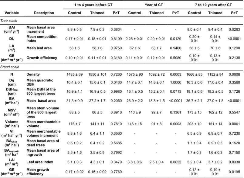
Tree scaleBAI that was calculated over a short period prior to thinning was similar between treatments (P = 0.6834, Table 2). For the period after thinning (7 to 10 years), BAI of thinned trees was significantly higher than that of control trees (P = 0.0283). Intensity of competition, which was evaluated using the mean value of DI4, was significantly
lower in thinned plots after CT (P < 0.0001), whereas it was similar prior to treatment (P = 0.6199).
Table 2 Mean stand characteristics (± standard error) of control and thinned plots before, after and seven
to ten years after thinning
1 to 4 years before CT Year of CT 7 to 10 years after CT
Variable Description Control Thinned P>T Control Thinned P>T Control Thinned P>T
Tree scale
BAI
(cm2 yr-1) Mean basal area increment 8.8 ± 0.3 7.9 ± 0.3 0.6834 - - - 8.0 ± 0.4 9.4 ± 0.4 0.0283 DI4 Mean competition index 0.17 ± 0.01 0.18 ± 0.01 0.6199 0.25 ± 0.01 0.20 ± 0.01 0.0129 0.20 ± 0.01 0.14 ± 0.01 <0.0001 LA
(m2) Mean leaf area 58 ± 6 58 ± 6 0.9750 62 ± 6 63 ± 7 0.9466 58 ± 5 70 ± 6 0.1298 GE (dm3 m-2 yr-1) Growth efficiency 0.10 ± 0.01 0.11 ± 0.01 0.3180 0.11 ± 0.01 0.12 ± 0.01 0.5080 0.10 ± 0.01 0.13 ± 0.01 0.2130 Stand scale N Density 1485 ± 69 1550 ± 101 0.7260 1575 ± 90 1092 ± 72 0.0003 1666 ± 85 1152 ± 84 0.0008 Dq (cm) Mean quadratic DBH 16.4 ± 0.1 15.0 ± 0.1 0.0480 14.7 ± 0.1 14.8 ± 0.1 1.0000 16.3 ± 0.6 17.0 ± 0.4 0.3560 DBH800
(cm) Mean DBH of the 800 largest trees 16.9 ± 1.1 16.9 ± 0.5 0.9980 16.4 ± 0.5 15.2 ± 0.4 0.0713 19.1 ± 0.6 18.2 ± 0.5 0.1726 BA
(m2 ha-1) Mean basal area 31.3 ± 0.9 27.2 ± 1.7 0.2060 26.9 ± 2.2 18.8 ± 1.5 <0.0001 36.7 ± 2.1 27.0 ± 1.8 <0.0001 MSV
(dm3 st-1)
Mean stem volume of the 800 largest
trees 88 ± 5 86 ± 5 0.8910 110 ± 9 92 ± 7 0.1361 173 ± 15 162 ± 12 0.5547 Volume
(m3 ha-1) Mean merchantable volume 176 ± 7 141 ± 11 0.7810 146 ± 15 91 ± 8 0.0003 203 ± 19 151 ± 14 0.0061 VI
(m3 ha-1 yr-1)
Mean merchantable
volume increment 8.8 ± 1.6 6.4 ± 1.1 0.3660 - - - 6.5 ± 0.9 6.9 ± 0.7 0.7230 BADead
(m2 ha-1) Mean basal area of dead trees 0.5 ± 0.2 0.4 ± 0.2 0.5685 - - - 1.7 ± 0.4 0.9 ± 0.3 0.1520 BAIngrowth
(m2 ha-1
Mean basal area of
ingrowth 5.5 ± 1.5 3.5 ± 0.9 0.7992 - - - 1.7 ± 0.3 1.6 ± 0.3 0.7150
LAI
(m2 m-2) Leaf area index 5.1 ± 0.3 4.3 ± 0.1 0.3470 3.8 ± 0.6 2.5 ± 0.4 0.0652 5.2 ± 0.4 3.7 ± 0.2 0.0330 GE (dm3 m-2 yr-1) Mean growth efficiency 0.17 ± 0.02 0.15 ± 0.02 0.7769 - - - 0.13 ± 0.01 0.19 ± 0.01 0.0195
19
Note: All values were computed using information of 16 plots per treatment except for the period before CT for which only 7 plots per treatment were available. LA and GE at the tree scale were computed using 64cored trees per treatment for each of the three periods.
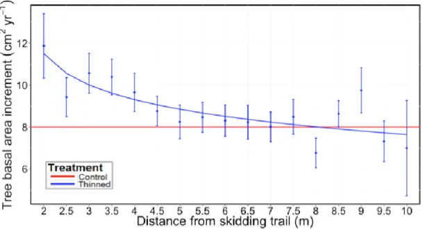
Post-thinning tree BAI decreased with increasing distance from the nearest skid trail (Eq. 10, R2 = 0.12, RMSE = 0.6106). For trees that were located more than 5 m away
from a trail, this effect became negligible as mean tree BAI approached that of trees in control plots (Fig. 2).
BAI = 12.81 – 1.37 log (Dist) [10]
where Dist is the shortest distance between a tree and a skid trail (m).
Figure 2 Tree basal area increment (BAI) as a function of distance from the nearest skidding trail. BAI
was calculated for a period of 7 to 10 years after thinning. Each point is the mean increment of 10 to 40 trees and the bars correspond to standard errors.
To evaluate whether tree LA was affected by the distance from the nearest skid trail, we first calibrated relationships between the number of growth rings in the sapwood and tree age using an age range covering 11 to 65 years for balsam fir (Eq. 11, n = 168, R2 = 0.33, RMSE = 0.3208) and 12 to 57 years for red spruce (Eq. 12, n = 66, R2
= 0.79, RMSE = 0.2407). Site index and tree social status were tested as covariates in these models, but they did not have a significant effect on the number of growth rings in sapwood (GRSA):
20
Balsam fir Ln GRSA = 0.652 + 0.470 Ln (Age) [11]
Red spruce Ln GRSA = 0.642 + 0.530 Ln (Age) [12]
Even if a fair part of the variation of GRSA remained unexplained, equations 11 and
12 were associated with unbiased residuals and were thus used to estimate past leaf area of both tree species using specific relationships between leaf area and sapwood area. Tree LA at any year after CT was best explained by LA at time of thinning (LA0),
tree social status (SS), and the interaction between the time that had elapsed since thinning (T) and distance from the nearest skid trail (Eq. 13, R2 = 0.85, RMSE =
0.3610).
Ln (LA) = 3.46 + 0.01 LA0 + a T · Location + b SS [13]
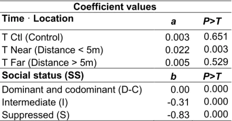
where a and b are regression coefficients that are indicated in Table 3.
According to the observed effect of distance from the nearest skid trail on tree BAI (Fig. 2), we used Eq. 13 for three categories of tree: control trees and thinned trees that were located within and outside a 5-m strip along skidding trails. Codominant trees had the largest LA, which was similar to that of dominant trees, but significantly higher than that of intermediate and suppressed trees (Table 3).
Table 3 Coefficient values for Eq. 13
Coefficient values Time · Location a P>T T Ctl (Control) 0.003 0.651 T Near (Distance < 5m) 0.022 0.003 T Far (Distance > 5m) 0.005 0.529 Social status (SS) b P>T
Dominant and codominant (D-C) 0.00 0.000
Intermediate (I) -0.31 0.000
Suppressed (S) -0.83 0.000
Note: For SS, the coefficients of dominant and codominant trees, which were statistically similar, were the reference value.
LA of trees that were located near skid trails increased linearly after CT, and based on confidence intervals, was significantly larger than that of control trees immediately
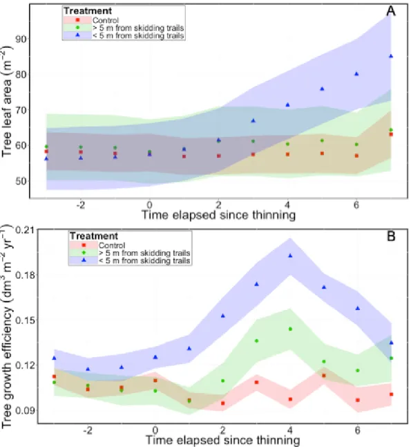
21 after the fourth year following treatment (Fig. 3A). This period corresponded to the maximum GE values for all thinned trees, whether they were within or outside a 5-m strip along skid trails (Fig. 3B). GE of thinned trees that were located less than 5 m from skid trails was higher than that of thinned trees located further away (Fig. 3B).
Figure 3 Temporal changes of tree leaf area (A) and growth efficiency (B) in control plots and for two
distance classes from the nearest skidding trail in thinned plots. Shaded areas correspond to the confidence interval of each tree category.
The preceding results suggest that competition indices that take into account the distance from skid trails should be more efficient in explaining tree growth than distance-independent competition indices. Using the optimum competition radius of 4
22
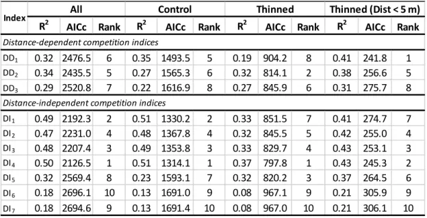
m, we compared distance-dependent and distance-independent indices on a subset of trees, for which the 4-m radius could be computed (575 trees), i.e., by excluding trees closer than 4 m from the inventoried zone boundaries. When we considered only trees that were located in the 5-m strip along a skid trail, we found that the distance-dependent index DD1 performed better than all other competition indices for predicting
tree basal area increment (Table 4). When we considered all trees in the sampling plots, we found that distance-independent competition indices generally outperformed distance-dependent indices, even in thinned plots where tree removal created heterogeneous tree distributions (Table 4). The best overall index was DI4, which
represents a measure of the area that is potentially available for a tree considering the proportional contribution of this tree to plot basal area (Tomé and Burkhart 1989).
Table 4 Statistics of competition index models fitted according to Eq. 3
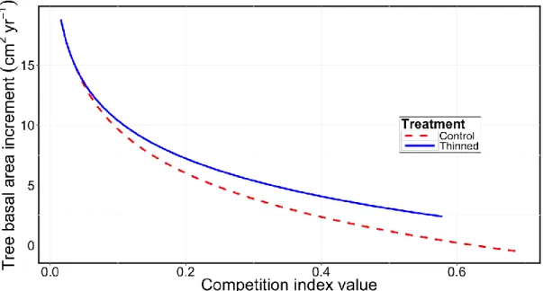
Using the competition index that was most closely related to tree growth (DI4), we
found that tree BAI decreased with increasing values of the competition index, but this decrease was less pronounced for thinned than for unthinned trees (Fig. 4). In addition, spruce trees had a slightly lower BAI compared to fir trees (P = 0.0442; Eq. 14, R2 = 0.50, RMSE = 0.5719).
Ln BAI = 2.77 – 0.10 Sp – 4.81 DI4·THN – 3.85 DI4·CTL [14]
where THN is for thinned trees and CTL for control trees.
R2 AICc Rank R2 AICc Rank R2 AICc Rank R2 AICc Rank
DD1 0.32 2476.5 6 0.35 1493.5 5 0.19 904.2 8 0.41 241.8 1 DD2 0.34 2435.5 5 0.27 1565.3 6 0.32 814.1 2 0.38 256.6 5 DD3 0.29 2520.8 7 0.22 1616.9 8 0.27 845.9 6 0.31 275.7 8 DI1 0.49 2192.3 2 0.51 1330.2 2 0.33 851.5 7 0.41 274.7 7 DI2 0.47 2231.0 4 0.48 1367.8 4 0.32 845.5 5 0.42 255.0 4 DI3 0.48 2207.4 3 0.49 1353.8 3 0.33 829.7 4 0.43 253.1 3 DI4 0.50 2126.5 1 0.51 1314.1 1 0.37 797.8 1 0.43 245.3 2 DI5 0.32 2569.4 8 0.23 1593.1 7 0.32 820.2 3 0.37 264.5 6 DI6 0.18 2696.1 10 0.13 1691.0 9 0.08 967.1 9 0.21 305.9 9 DI7 0.18 2694.6 9 0.13 1691.4 10 0.08 967.0 10 0.21 306.1 10 Distance-independent competition indices
Index All Control Thinned Thinned (Dist < 5 m)
23
Figure 4 Predicted tree basal area increment as a function of the competition index DI4; thinning is for
balsam fir trees.
Stand scale
To compute growth efficiency at the stand scale, LA for spruce and fir trees that had not been cored was estimated with the following equation (R2 = 0.65, RMSE = 0.4200):
Ln LA = 0.580 + 0.005 DBH + 0.530 Ln (CSA) + 0.470 Sp [15]
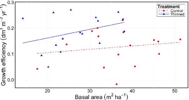
Thinning significantly increased the periodic amount of wood that was produced per unit leaf area, i.e., GE, by 45 % (Fig. 5). GE tended to increase with increasing basal area that was measured in 2014 for both control and thinned plots, but this trend was not statistically significant. Leaf area index (LAI) decreased by 2 m2 m-2 about 7 to 10
years after thinning (Table 2). Yet mean DBH of the 800 largest trees per hectare (DBH800), which corresponds approximately to the number of trees that were harvested
at maturity, did not differ between treatments, either immediately following thinning, or 7 to 10 years afterwards (Table 2). Accordingly, no significant differences between treatments were detected for mean stem volume and stand merchantable volume increment. Thinning slightly reduced tree mortality compared to control plots, but this difference was not statistically different. There was also no evidence that CT increased the basal area of ingrowth (Table 2).
24
Figure 5 Growth efficiency as a function of basal area in 2014 for thinned and unthinned stands. Each
point corresponds to GE computed at the plot level.
Temporal changes in merchantable stand volume for each pair of plots followed statistically parallel trajectories with volume increments averaging of 6.7 m3 ha-1 yr-1
for both thinned and unthinned plots. Merchantable standing volume of these stands was best predicted by time-since-thinning (T), the basal area prior to thinning (BA0),
and the leaf area index before thinning (LAI0), whereas other stand and site variables
did not improve the model (Eq. 16, R2 = 0.81, RMSE = 29.79):
V = 6.7 T + 4.2 BA0 + 12.1 LAI0 - 39.7 CT [16]
Accordingly, the relative difference in volume (RVD) between thinned and control plots was not statistically different from zero (P = 0.2580) when all trees from the treated plots were used in the calculations, indicating parallel volume trajectories. However, using RVD computed only with trees within 5-m strips along the skid trails, volume trajectories were found divergent (P = 0.0092). Despite the overall parallel volume trajectories of thinned and control plots, some of the 16 pairs of study plots showed slightly divergent and convergent volume trajectories (Fig. 5). Using the RVD between the control and thinned plots in each pair, we related these differences with other variables, such as the proportion of basal area removed and the proportion of
25 the thinned plot area that was covered by a skid trail. Since none of these variables was significantly related to RVD, the deviations from parallelism appeared to be incidental or at least unrelated to site conditions and to the tested thinning patterns. Finally, some of the pairs of plots show small differences in merchantable volume immediately after thinning application (e.g. blocks 2, 4, 6 and 13 in Fig. 5). These small differences are explained by high volume stocking of thinned plots before treatment relative to control plots rather than by low thinning intensity.
26
Discussion
The spatial coordinates of trees and skid trails allowed us to detect clear tree growth responses to the treatment seven to ten years after commercial thinning. Indeed, because the application of CT mostly consisted of removing trees in skid trails and at short distances on either side of these trails, significant tree basal area and leaf area responses to thinning were limited to the trees that were located within 5-m wide strips on either side of the trails. The quantity of wood that was produced per unit leaf area at the overall plot level was significantly higher in thinned than in control plots, but this seemed insufficient to increase the stand volume, as evidenced by the parallel trajectories of merchantable volume over time between most pairs of thinned and control plots.
Spatial effects
We detected a spatial response pattern among trees in thinned plots, which was related to the creation of gaps that were formed by skid trails and by nearby tree removal. This was consistent with the observations of Roberts and Harrington (2008) and Genet and Pothier (2013). Consistent with our second hypothesis, BAI of thinned trees increased with decreasing distance from the nearest skid trail (Fig. 2). Genet and Pothier (2013) also found that relative diameter increment of trees with a DBH < 14 cm was stimulated near logging trails after partial cutting in coniferous stands. In our study, growth improvement was mainly present in the first 5 m from a trail, regardless of tree size. Beyond this threshold distance, BAI of trees appeared to stabilize around its lowest value plateau, which was similar to that of control trees (8 cm2 yr-1).
Therefore, we can conclude that restricting tree removal to only few meters from skid trails prevented the extension of positive effects of thinning to the entire treated stand.
Our results support our first hypothesis stating that the causes of tree growth response to CT shift over time from wood production efficiency to resource acquisition. Indeed, we observed an increase in GE as soon as the year of thinning for trees that were located near skid trails (Fig. 3B), suggesting that acclimation of trees to CT first increased the efficiency of a given leaf area to produce wood in response to higher light availability. This difference in GE between thinned and unthinned trees continued to increase until the fourth year after thinning, at which time it began to decrease as a
27 significant difference in LA first appeared (Fig. 3A). Accordingly, increased access to solar radiation is an important determinant of leaf area expansion (Binkley et al., 2010; Omari et al., 2016). Creation of gaps in and beside skid trails resulted in higher light availability for nearby residual trees, which stimulated wood production per unit leaf area over the short-term and crown expansion over the mid-term. This overall acclimation of trees to improved light availability explains improved stemwood growth at the tree level (Brix, 1983; Vose and Allen, 1988; DeRose and Seymour, 2010). This effect is especially noticeable for dominant and codominant trees, which have the largest increase in LA.
Non-spatial effects
In spite of the spatial effects of skid trails on tree growth, distance-dependent competition indices did not perform better than distance-independent indices in predicting BAI after thinning for thinned and unthinned trees altogether (Table 4), as was observed by Roberts and Harrington (2008). Indeed, for a distance-dependent index to be more efficient than distance-independent indices, only trees within 5-m strips along the skid trails needed to be considered in the analysis. Overall better performance of distance-independent indices is likely related to the relatively low mass of trees within 5-m strips along skid trails, which corresponds to 35 % of the remaining trees in all thinned plots (185 of 575 trees). This result has practical importance since distance-independent indices have the advantage of being computable from usual inventory data, which is not the case for distance-dependent indices.
The distance-independent competition index DI4 was the overall best predictor of
stemwood growth. Thinning significantly reduced overall stand competition, which in turn significantly reduced DI4 values (Table 2) and increased tree growth (Fig. 4).
Reduction in competition decreased conflicts between trees for the acquisition of the same pool of available resources (Larocque et al., 2013). Furthermore, DI4 seems to
be an adequate index for evaluating the effect of silvicultural treatments at the tree- and stand-levels, given that it refers to stand density and to a dominance ratio that was based on BA (Jack and Long, 1996). It is the only index that including both a tree- and a stand-level variable, which seems necessary for adequately describing the competition in thinned and unthinned stands. Yet the relationship between DI4 and
28
between thinned and unthinned plots was similar at low competition values, trees had increasingly larger BAI in thinned than in control plots with increasing DI4 values. This
growth advantage of thinned plots for a given level of competition is likely related to the greater GE of trees near skid trails. Thus, the interaction between DI4 and
treatment suggests that effects of spatial heterogeneity in thinned stands were strong enough to influence average tree growth (Fig. 4). Last, the BAI prediction model revealed that for the same competition intensity, growth of balsam fir was slightly greater than that of red spruce, which accords with the generally observed faster development of balsam fir in coniferous stands of northeastern North America (Day, 2000; Dumais and Prévost, 2014).
Commercial thinning significantly decreased LAI at the stand level (Table 2), but this response was compensated by an increase of about 45 % in annual stemwood production per unit leaf area (Fig. 5). This increase in GE after thinning could have been larger, if we were capable of evaluating the response of all tree biomass compartments. For example, Vincent et al. (2009) found that root biomass growth of black spruce was improved in the first four years following thinning, whereas stem growth response was delayed and still ongoing after 10 years. Apart from effects on tree growth, GE also provided an index of stand vigour or its sensitivity to environmental stresses (Waring, 1983). For example, a detectable benefit of CT on
GE
is the
increased resistance of balsam fir to defoliation, especially by the sprucebudworm (Choristoneura fumiferana [Clemens]) (Bauce, 1996).
A frequent assumption is that CT can increase the total stand production (the combined volume of thinning and final harvest) by offsetting potential mortality (Nyland, 2002). This would mainly be the result of the removal of weak trees, which are susceptible to attacks by pests and pathogens, while retaining vigorous trees (Marshall and Curtis, 2002; Mäkinen and Isomäki, 2004). Thinning did not significantly reduce losses due to mortality (Table 2), which likely contributed to similar yields between thinned and unthinned plots (Fig. 6). The inability of thinning to significantly reduce tree mortality compared to control plots could be related to the relatively large proportion of thinned plots that was not effectively thinned, as suggested by the tree growth improvement that was limited to the 5-m strips along the trails. These findings are consistent with the most accepted outcome of thinning, which predicts a parallel
29 response to thinning (Zeide, 2001). A major explanation of parallel trajectories of merchantable volume over time that were observed in this case study is that the passage of machinery requires relatively wide trails where every tree is harvested. These trails lead to a reduction of about 20 % of the basal area in a treatment that targets an overall removal of 35 %. This leaves only 15 % for which a true stem selection procedure was possible, and results show that this was concentrated near the trails. Accordingly, mechanized thinning treatments rarely lead to gains in merchantable volume over a full rotation (Smith et al., 1997; Marshall and Curtis, 2002). Our third hypothesis stated that departures from parallelism (divergence) in volume trajectories between control and thinned plots would increase with increasing thinning intensity or area occupied by skid trails. This hypothesis received little support from our analysis, most likely because of our limited sample size or range of thinning intensity or proportion of the area that was effectively thinned. Indeed, when we considered only the part of the stand that was effectively thinned, i.e. the 5-m strips along the skid trails, the volume trajectories were found divergent.
Another assumed effect of thinning that is also used to justify its application, is the improvement of tree size and quality (Mäkinen and Isomäki, 2004; Karlsson, 2006; Pelletier and Pitt, 2008). The study stands did not produce this expected outcome, as CT did not significantly stimulate increases in either DBH800, or mean stem volume.
This suggests that 7 to 10 years after treatment, thinned and unthinned stands should have a similar level of product recovery and, therefore, value (Auty et al., 2014). In addition to the relatively short monitoring period, these results can again be explained by the fact that tree harvesting was mainly done in and around trails, which resulted in a similar level of removal within each size class and a growth response that was limited to a small proportion of trees located near the trails.
Silvicultural implications
Maximizing timber production by CT typically involves the application of light but frequent thinning (Marshall and Curtis, 2002; Mäkinen and Isomäki, 2004). This strategy can be applied in small woodlots or in experimental trials where manual harvesting and careful forwarding are possible (Soucy et al., 2012; Barrette and Tremblay, 2015). However, the operational deployment of thinning over large areas requires mechanized operations with which this strategy is not compatible. Indeed,
30
mechanized operations require trails for machinery passage, which may form unproductive areas if they are too large (Long and Smith, 1992). Also, our observations of localized tree growth improvement along skid trails suggest that mechanized applications of CT should be adjusted to expand its positive effects to a larger proportion of the stand. The first adjustment would be to reduce trail width in order to accelerate canopy closure and, thus, ensure full site occupancy by trees. This would be possible using small harvesters and forwarders. Second, we suggest that the maximum boom reach of the harvester be used to remove trees as far as possible from skid trails to increase the proportion of released trees. If the reach of the harvester is limited, we suggest considering alternative harvesting systems such as ghost trails within which only the harvester is allowed to circulate to efficiently access interior of strips between skid trails.