Lanczos-type solvers for nonsymmetric linear systems of equations

Lanczos-type solvers for nonsymmetric

linear systems of equations

Martin H. Gutknecht

Swiss Center for Scientific Computing ETH-Zentrum, CH-8092 Zurich, Switzerland

E-mail: mhg@scsc.ethz.ch

Among the iterative methods for solving large linear systems with a sparse (or, possibly, structured) nonsymmetric matrix, those that are based on the Lanczos process feature short recurrences for the generation of the Krylov space. This means low cost and low memory requirement. This review article introduces the reader not only to the basic forms of the Lanczos process and some of the related theory, but also describes in detail a number of solvers that are based on it, including those that are considered to be the most efficient ones. Possible breakdowns of the algorithms and ways to cure them by look-ahead are also discussed.

272 M. H. GUTKNECHT

C O N T E N T S

1 Introduction 272 2 The unsymmetric Lanczos or BlO algorithm 280 3 Termination, breakdowns and convergence 288 4 The BlORES form of the BlCG method 292 5 The QMR solution of a linear system 301 6 Variations of the Lanczos BlO algorithm 309 7 Coupled recurrences: the BlOC algorithm 314 8 The BlOMlN form of the BlCG method 319 9 The BlODm form of the BlCG method;

comparison 323 10 Alternative ways to apply the QMR approach

to BlCG 328 11 Preconditioning 330 12 Lanczos and direction polynomials 332 13 The Lanczos process for polynomials:

the Stieltjes procedure 340 14 The biconjugate gradient squared method 342 15 The transpose-free QMR algorithm 349 16 Lanczos-type product methods 352 17 Smoothing processes 365 18 Accuracy considerations 370 19 Look-ahead Lanczos algorithms 375 20 Outlook 388 References 389

1. Introduction

The task of solving huge sparse systems of linear equations comes up in many if not most large-scale problems of scientific computing. In fact, if tasks were judged according to hours spent on them on high-performance computers, the one of solving linear systems might be by far the most im-portant one. There are two types of approach: direct methods, which are basically ingenious variations of Gaussian elimination, and iterative ones, which come in many flavours. The latter are the clear winners when we have to solve equations arising from the discretization of three-dimensional partial differential equations, while for two-dimensional problems none of the two approaches can claim to be superior in general.

Among the many existing iterative methods, those based on the Lanczos process - and we consider the conjugate gradient (CG) method to be in-cluded in this class - are definitely among the most effective ones. For symmetric positive definite systems, CG is normally the best choice, and

arguments among users are restricted to which preconditioning technique to use and whether it is worthwhile, or even necessary, to combine the method with other techniques such as domain decomposition or multigrid.

For nonsymmetric (or, more correctly, non-Hermitian) systems it would be hard to make a generally accepted recommendation. There are dozens of algorithms that are generalizations of CG or are at least related to it. They fall basically into two classes: (i) methods based on orthogonalization, many of which feature a minimality property of the residuals with respect to some norm, but have to make use of long recurrences involving all pre-viously found iterates and residuals (or direction vectors), unless truncated or restarted, in which case the optimality is lost; and (ii) methods based on biorthogonalization (or, duality) that feature short recurrences and a competitive speed of convergence. It is the latter class that is the topic of this article. The gain in memory requirement and computational effort that comes from short recurrences is often crucial for making a problem solv-able. While computers get faster and memory cheaper, users turn to bigger problems, so that efficient methods become more rather than less important. The application of recursive biorthogonalization to the numerical solu-tion of eigenvalue problems and linear systems goes back to Lanczos (1950, 1952) and is therefore referred to as the Lanczos process. In its basic form, the process generates a pair of biorthogonal (or, dual) bases for a pair of Krylov spaces, one generated by the coefficient matrix A and the other by its Hermitian transpose or adjoint A*. This process features a three-term recurrence and is here called Lanczos biorthogonalization or BlO algorithm (see Section 2). A variation of it, described in the second Lanczos paper, applies instead a pair of coupled two-term recurrences and is here referred to as BlOC algorithm, because it produces additionally a second pair of biconjugate bases (see Section 7). Both these algorithms can be applied for solving a linear system A x = b or for finding a part of the spectrum of A. For the eigenvalue problem it has so far been standard to use the BlO algorithm, but there are indications that this may change in the future (see the comments in Section 7).

The emphasis here is neither on eigenvalue problems nor on symmetric linear systems, but on solving nonsymmetric systems. Although the determ-ination of eigenvalues is based on the same process, its application to this problem has a different flavour and is well known for additional numerical difficulties. Moreover, for the eigenvalue problem, the spectrum of a tridiag-onal matrix has to be determined in a postprocessing step. For generality, our formulations include complex systems, although the methods are mainly applied to real data.

For symmetric positive definite systems, the Lanczos process is equival-ent to the conjugate gradiequival-ent (CG) method of Hestenes and Stiefel (1952), which has been well understood for a long time and is widely treated in the

274 M. H. GUTKNECHT

literature. Related algorithms for indefinite symmetric systems are also well known. Therefore, we can concentrate on the nonsymmetric case.

For an annotated bibliography of the early work on the CG and the Lanczos methods we refer to Golub and O'Leary (1989). The two Lanczos papers are briefly reviewed in Stewart (1994).

There are several ways of solving linear systems iteratively with the Lan-czos process. Like any other Krylov space method, the LanLan-czos process generates a nested sequence of Krylov subspaces1 Kn: at each step, the

so far created basis {yo,... , yn_ i } is augmented by a new (right) Lanczos

vector yn that is a linear combination of A yn_ i and the old basis. The

starting vector yo is the residual of some initial approximation xo, that is, yo := b —Axo. The nth approximation xn (the nth 'iterate') is then chosen

to have a representation

n

x

= x

+ Yl yj

o

x

- x

G K.

. (1.1)

This is what characterizes a Krylov space solver. Note, however, that the

algorithms to be discussed will not make use of this representation since it

would require us to store the whole Krylov space basis. It is a feature of

all competitive Lanczos-type solvers that the iterates can be obtained with

short recurrences.

The Lanczos process is special in that it generates two nested sequences of

Krylov spaces, one, {/C

}, from A and some yo, the other, {K

} from A* and

some yo- The iterates of the classical Lanczos-type solver, the biconjugate

gradient (BlCG) method, are then characterized by K.

_L r

, where r

:=

b — Ax

is the nth residual.

In the 'symmetric case', when A is Hermitian and yo = yo>

that K

=

K

(for all n), this orthogonality condition is a Galerkin condition, and the

method reduces to the conjugate gradient (CG) method, which is known to

minimize the error in the A-norm when the matrix is positive definite. Of

course, the minimization is subject to the condition (1.1). By replacing in

the symmetric case the orthogonality by A-orthogonality, that is, imposing

K

_L Ar

, we obtain the conjugate residual (CR) or minimum residual

method - a particular algorithm due to Paige and Saunders (1975) is called

MINRES,

see Section 5 - with the property that the residual is minimized.

As a consequence, the norm of the residuals decreases monotonically.

For non-Hermitian matrices A the two Krylov spaces are different, and

K,

J_ r

becomes a Petrov-Galerkin condition. In the BlCG method the

short recurrences of CG and CR survive, but, unfortunately, the error and

residual minimization properties are lost. In fact, in practice the norm of

1 _{Throughout the paper we refer for simplicity mostly to Krylov spaces, not subspaces,}

the residuals sometimes increases suddenly by orders of magnitude, but also reduces soon after to the previous level. This is referred to as a peak in the residual norm plot, and when this happens several times in an example, BiCG is said to have an erratic convergence behaviour.

There are two good ways to achieve a smoother residual norm plot of BiCG. First, one can pipe the iterates xn and the residuals rn of BiCG

through a simple smoothing process that determines smoothed iterates xn

and rn according to

xn := xn_i(l - 0n) + xn9n, rn := rn_ i ( l - 0n) + rn0n,

where 9n is chosen such that the 2-norm of rn is as small as possible. This

simple recursive weighting process is very effective. It was proposed by Schonauer (1987) and further investigated by Weiss (1990). Now it is re-ferred to as minimal residual (MR) smoothing; we will discuss it in Sec-tion 17.

An alternative is the quasi-minimal residual (QMR) method of Freund and Nachtigal (1991), which does not use the BiCG iterates directly, but only the basis {yj} of JCn that is generated by the Lanczos process. The

basic idea is to determine iterates xn so that the coordinate vector of their

residual with respect to the Lanczos basis has minimum length. This turns out to be a least squares problem with an (n + 1) x n tridiagonal matrix, the same problem as in MINRES; see Section 5.

QMR can also be understood as a harmonic mean smoothing process for the residual norm plot, and therefore, theoretically, neither QMR nor MR smoothing can really speed up the convergence considerably. In prac-tice, however, it often happens that straightforward implementations of the BiCG method converge more slowly than a carefully implemented QMR algorithm (or not at all).

At this point we should add that there are various ways to realize the BiCG method (see Sections 4, 8 9), and that they all allow us to com-bine it with a smoothing process. In theory, the various algorithms are mathematically nearly equivalent, but with respect to round-off they differ. And round-off is indeed a serious problem for all Lanczos process based al-gorithms with short recurrences: when building up the dual bases we only enforce the orthogonality to the two previous vectors; the orthogonality to the earlier vectors is inherited and, with time, is more and more lost due to round-off. We will discuss this and other issues of finite precision arithmetic briefly in Section 18.

In contrast to smoothing, an idea due to Sonneveld (1989) really increases the speed of convergence. At once, it eliminates the following two disad-vantages of the nonsymmetric Lanczos process: first, in addition to the subroutine for the product Ax that is required by all Krylov space solv-ers, BiCG also needs one for A*x; second, each step of BiCG increases

276 M. H. GUTKNECHT

the dimension of both K,n and Kn by one and, naturally, needs two

matrix-vector multiplications to do so, but only one of them helps to reduce the approximation error by increasing the dimension of the approximation space. To explain Sonneveld's idea we note that every vector in the Krylov space

Kn+i has a representation of the form pn(A)yo with a polynomial of degree

at most n. In the standard version of the BlCG method, the basis vectors generated are linked by this polynomial:

yn = Pn(A)y0, yn = pn(A*)y0.

Here, the bar denotes complex conjugation of the coefficients. Since yn

happens to be the residual rn of xn, pn is actually the residual polynomial.

Sonneveld found with his conjugate gradient squared (CGS) algorithm a method where the nth residual is instead given by rn = p^(A)yo G

K.2n-Per step it increases the Krylov space by two dimensions. Moreover, the transpose or adjoint matrix is no longer needed. In practice, the conver-gence is indeed typically nearly twice as fast as for BlCG, and thus also in terms of matrix-vector multiplications the method is nearly twice as effect-ive. However, it turns out that the convergence is even more erratic. We will refer to this method more appropriately as biconjugate gradient squared (BlCGS) method and treat various forms of it in Section 14.

To get smoother convergence, van der Vorst (1992) modified the ap-proach in his B I C G S T A B algorithm by choosing residuals of the form rn = pn(A)tn(A)yo G K.2n, where the polynomials tn are built up in factored form,

with a new zero being added in each step in such a way that the residual undergoes a one-dimensional minimization process. This method was soon enhanced further and became the germ of a group of methods that one might call the B I C G S T A B family. It includes B I C G S T A B 2 with two-dimensional minimization every other step, and the more general B I C G S T A B ( ^ ) with

£-dimensional minimization after a compound step that costs 2£ matrix-vector products and increases the dimension of the Krylov space by 2£. The B I C G -STAB family is a subset of an even larger class, the Lanczos-type product methods (LTPMs), which are characterized by residual polynomials that are products of a Lanczos polynomial pn and another polynomial tn of the same

degree. All LTPMs are transpose-free and gain one dimension of the Krylov space per matrix-vector multiplication. Basically an infinite number of such methods exist, but it is not so easy to find one that can outperform, say,

B I C G S T A B 2 . One that seems to be slightly better is based on the same idea as B I C G S T A B 2 and, in fact, requires only the modification of a single condition in the code. We call it B i C G x M R 2 . It does a two-dimensional minimization in each step. LTPMs in general and the examples mentioned here are discussed in Section 16.

Another good idea is to apply the QMR approach suitably to BlCGS. The resulting transpose-free QMR (TFQMR) algorithm of Freund (1993)

can compete in efficiency with the best LTPMs; we treat it in Section 15. It is also possible to apply the QMR approach to LTPMs; see the introduction of Section 16 for references.

A disadvantage of Krylov space methods based on the Lanczos process is that they can break down for several reasons (even in exact arithmetic). Particularly troublesome are the 'serious' Lanczos breakdowns that occur when

(yn,yn)=0, but y n ^ ° , y n ^ o .

Though true ('exact') breakdowns are extremely unlikely (except in

con-trived or specially structured examples), near-breakdowns can be (but need

not be) the cause for an interruption or a slow-down of the convergence.

These breakdowns were surely among the reasons why the BiCG method

was rarely used over decades. However, as problem sizes grew, it became

more and more important to have a method with short recurrences.

Fortu-nately, it turned out that there is a mathematically correct way to

circum-vent both exact and near-breakdowns. The first to come up with such a

procedure for the BiO algorithm for eigenvalue computations were Parlett,

Taylor and Liu (1985), who also coined the term 'look-ahead'. In their view,

this was a generalization of the two-sided Gram-Schmidt algorithm. In 1988

look-ahead was rediscovered by Gutknecht from a completely different

per-spective: for him, look-ahead was a translation of general recurrences in the

Pade table, and a realization of what Gragg (1974) had indicated in a few

lines long before. Although classical Pade and continued fraction theory

put no emphasis on singular cases, the recurrences for what corresponds

to an exact breakdown had been known for a long time. Moreover, it was

possible to generalize them in order to treat near-breakdowns. This theory

and the application to several versions of the BiCG method are compiled

in Gutknecht (1992, 1994a). The careful implementation and the numerical

tests of Freund, Gutknecht and Nachtigal (1993) ultimately proved, that all

this can be turned into robust and efficient algorithms. Many other authors

have also contributed to look-ahead Lanczos algorithms; see our references

in Section 19. Moreover, the basic idea can be adapted to many other related

recurrences in numerical analysis.

Here, we describe in Section 3 in detail the various ways in which the

BiO algorithm can break down or terminate. Throughout the manuscript

we then point out under which conditions the other algorithms break down.

Although breakdowns are rare, knowing where and why they occur is

im-portant for learning how to avoid them and for gaining a full understanding

of Lanczos-type algorithms. Quality software should be able to cope with

breakdowns, or at least indicate to the user when a critical situation occurs.

Seemingly, we only indicate exact breakdowns, but, of course, to include

near-breakdowns the conditions '= o' and '= 0' just have to be replaced

278 M. H. GUTKNECHT

by other appropriate conditions. In practice, however, the question of what 'appropriate' means is not always so easy to answer. It is briefly touched on in Section 19.

The derivations of the look-ahead BlO and BlOC algorithms we present are based on the interpretation as two-sided Gram-Schmidt process. The algorithms themselves are improved versions with reduced memory require-ment. The look-ahead BlO algorithm makes use of a trick hidden in Freund and Zha (1993) and pointed out in Hochbruck (1996). We establish this simplification in a few lines, making use of a result from Gutknecht (1992). For the look-ahead BlOC algorithm the simplification is due to Hochbruck (1996), but also proved here in a different way.

We give many pointers to the vast literature on Krylov space solvers based on the Lanczos process, but treating all the algorithms proposed is far beyond our scope. In fact, this literature has grown so much in the last few years that we have even had to limit the number of references. Moreover, there must exist papers we are unaware of. Our intention is mainly to give an easy introduction to the nonsymmetric Lanczos process and some of the linear system solvers based on it. We have tried in particular to explain the underlying ideas and to make clear the limitations and difficulties of this family of methods. We have chosen to treat those algorithms that we think are important for understanding, as well as those we think are among the most effective.

There are many aspects that are not covered or only briefly referred to. First of all, the important question of convergence and its deterioration due to numerical effects is touched on only superficially. Also, we do not give any numerical results, since giving a representative set would have required considerable time and space. In fact, while straightforward implementation of the algorithms requires little work, we believe that the production of quality software taking into account some of the possible enhancements we mention in Section 18 - not to speak of the look-ahead option that should be included - requires considerable effort. Testing and evaluating such software is not easy either, as simple examples do not show the effects of the enhance-ments, while complicated ones make it difficult to link causes and effects. To our knowledge, the best available software is Freund and Nachtigal's QM-RPACK, which is freely available from NETLIB, but is restricted to various forms of the Q M R and T F Q M R methods; see Freund and Nachtigal (1996). While we are aware that in practice preconditioning can improve the con-vergence of an iterative method dramatically and can reduce the overall costs, we describe only briefly in Section 11 how preconditioners can be in-tegrated into the algorithms, but not how they are found. For a survey of preconditioning techniques we refer, for example, to Saad (1996).

Also among the things we skip are the adaptations of the Lanczos method to systems with multiple right-hand sides. Recent work includes Aliaga,

Hernandez and Boley (1994) and Freund and Malhotra (1997), which is an extension of Ruhe's band Lanczos algorithm (Ruhe 1979) blended with QMR.

The Lanczos process is closely linked to other topics with the same math-ematical background, in particular, formal orthogonal polynomials, Pade approximation, continued fractions, the recursive solution of linear systems with Hankel matrix, and the partial realization problem of system theory. We discuss formal orthogonal polynomials (FOPs) briefly in Section 12, but the other topics are not touched on. For the Pade connection, which is very helpful for understanding breakdowns and the look-ahead approach to cure them, we refer to Gutknecht (19946) for a simple treatment. The relation-ship is described in much more detail and capitalized upon in Gutknecht (1992, 1994a), where Lanczos look-ahead for both the BlO and the BlOC process was introduced based on this connection. The relations between vari-ous look-ahead recurrences in the Pade table and variations of look-ahead Lanczos algorithms are also a topic of Hochbruck (1996). A fast Hankel solver based on look-ahead Lanczos was worked out in detail in Freund and Zha (1993). For the connection to the partial realization problem; see Boley (1994), Boley and Golub (1991), Golub, Kagstrom and Van Dooren (1992), and Parlett (1992).

In the wider neighbourhood of the Lanczos process we also find the Eu-clidean algorithm, Gauss quadrature, the matrix moment problem and its modified form, certain extrapolation methods, and the interpretation of con-jugate direction methods as a special form of Gauss elimination. But these subjects are not treated here.

A preliminary version of a few sections of this overview was presented as an invited talk at the Copper Mountain Conference on Iterative Methods 1990 and was printed in the Preliminary Proceedings distributed at the conference. The present Section 14 (plus some additional material) was made available on separate sheets at that conference. We refer here to these two sources as Gutknecht (1990).

Notation

Matrices and vectors are denoted by upper and lower case boldface letters. In particular, O and o are the zero matrix and vector, respectively. The transpose of A is AT; its conjugate transpose is A*. Blocks of block vec-tors and matrices are sometimes printed in roman instead of boldface. For coefficients and other scalars we normally choose lower case Greek letters. However, for polynomials (and some function values) we use lower case ro-man letters. Sets are denoted by calligraphic letters; for instance, Vn is the

280 M. H. GUTKNECHT

We write scalars on the right-hand side of vectors, for instance xa, so

that this product becomes a special case of matrix multiplication

. The

inner product in C^ is assumed to be defined by (x,y) := x*y, so that

(xa,y/3) = a(3(x,y). The symbol := is used both for definitions and for

algorithmic assignments.

To achieve a uniform nomenclature for the methods and algorithms we

consider, we have modified some of the denominations used by other authors

(but we also refer to the original name if the identity is not apparent). We

hope that this will help readers to find their way in the maze of Lanczos-type

solvers.

2. The unsymmetric Lanczos or BiO algorithm

In this section we describe the basic nonsymmetric Lanczos process that

generates a pair of biorthogonal vector sequences. These define a pair of

nested sequences of Krylov spaces, one generated by the given matrix or

operator A, the other by its Hermitian transpose A*. The Lanczos algorithm

is based on a successive extension of these two spaces, coupled with a

two-sided Gram-Schmidt process for the construction of dual bases for them.

The recurrence coefficients are the elements of a tridiagonal matrix that is,

in theory, similar to A if the algorithm does not stop early. In the next

section we will discuss the various ways in which the process can terminate

or break down.

2.1. Derivation of the BiO algorithm

Let A € C

be any real or complex N x N matrix, and let B be a

nonsingular matrix that commutes with A and is used to define the formal

(i.e., not necessarily symmetric definite) inner product (y,y)B

y*By

on C^ x C^. Orthogonality will usually be referred to with respect to

this formal inner product. For simplicity, we do not call it B-orthogonality,

except when this inaccuracy becomes misleading. However, we are mostly

interested in the case where B is the identity I and thus (y, y)B is the

ordinary Euclidean inner product of C^. The case B = A will also play a

role. Due to AB = BA we will have (y, Ay)s = (A*y, y)s • Finally, we

let yo, yo £ C

be two non-orthogonal initial vectors: (yo,yo)B ¥"

0-The Lanczos biorthogonalization (BiO) algorithm, called method of

min-imized iterations by Lanczos (1950, 1952), but often referred to as the

un-symmetric or two-sided Lanczos algorithm, is a process for generating two

finite sequences {y

}n=o

^ {yn}n=oi whose length v depends on A, B,

2

To see the rationale, think of the case where a turns out to be an inner product or where we generalize to block algorithms and a becomes a block of a vector.

yo, and yo, such that, for m, n = 0 , 1 , . . . , v — 1,

yn € K.n+i := span (y0, A y0, . . . , A " y0) ,

(2.1)

•= span (y0, A*yo,..., (A*)my0)

and

) if

= n.

'

K

and JC

are Krylov (sub)spaces of A and A*, respectively. The condition

(2.2) means that the sequences are biorthogonal. Their elements y

and y

are called right and left Lanczos vectors, respectively. In view of (2.1) y^

and yn can be expressed as

y

=Pn(A)y

, y

=p

(A*)y

, (2.3)

where p

and p

are polynomials of degree at most n into which A and A*

are substituted for the variable. We call p

the nth Lanczos polynomial^.

We will see in a moment that p

has exact degree n and that the sequence

{y

} can be chosen such that p

= p

, where p

is the polynomial with the

complex conjugate coefficients. In the general case, p

will be seen to be a

scalar multiple of p

.

The biorthogonal sequences of Lanczos vectors are constructed by a

two-sided version of the well-known Gram-Schmidt process, but the latter is not

applied to the bases used in the definition (2.1), since these are normally very

ill-conditioned, that is, close to linearly dependent. Instead, the vectors that

are orthogonalized are of the form Ay

and A*y

; that is, they are created

in each step from the most recently constructed pair by multiplication with

A and A*, respectively.

The length v of the sequences is determined by the impossibility of

ex-tending them such that the conditions (2.1) and (2.2) still hold with 6

^ 0.

We will discuss the various reasons for a termination or a breakdown of the

process below.

Clearly K.

\ I> IC

, K.

+\ 2 £n> and from (2.2) it follows that equality

cannot hold when n < v, since (y, y

)B = 0 for all y 6 K,

and (y

, Y)B = 0

for all y e K

, or, briefly,

n, Yn J-B £n, (2.4) but ICn+i JL-B yn, yn JLB /Cn +i. Consequently, for n = 1 , . . . , v - 1,

yn G K.n+i\K-n, yn G >Cn+i\JCn (2.5) 3

In classical analysis, depending on the normalization, the Lanczos polynomials are called Hankel polynomials or Hadamard polynomials, the latter being monic (Henrici

282 M. H. GUTKNECHT

(where the backslash denotes the set-theoretic difference), and thus

/Cn+i = s p a n ( yo, y i , . . . , yT l) , £«+i = span ( yo, y i , • • • ,yn)- (2.6)

Note that the relation on the left of (2.4) is equivalent to yn J_B* K-n, but

not to yn J_B K-m m general.

Prom (2.5) and (2.6) we conclude that for some complex constants Tk,n-i, Tk,n-i {k = 0 , . . . , n; n = 1 , . . . , v - 1)

ynTn,n-i = A * yn_ i — yn-iTn-i,n-i — • • • — y ^

where Tn^n-\ ^ 0 and Tn,n-\ ^ 0 can be chosen arbitrarily, for instance, for

normalizing yn and yn. The choice will of course affect the constants 6m

and the coefficients rn^m and Tn^m for m > n, but only in a transparent way.

For n = v, (2.7) can still be satisfied for any nonzero values of TVyV-\ and Tv,v-i by some y^ ± B * £V a nd some yu J_B fcu, but these two vectors may

be orthogonal to each other, so that (2.2) does not hold. In particular, one or even both may be the zero vector o. Nevertheless, (2.4) and (2.6)-(2.7) also hold for n = v.

For n < v, let us introduce the N x n matrices

Yn := [ y0 yi ••• yn- i ], Yn := [ yo yi ••• yn- i ], (2.8)

the diagonal matrices

and the n x n Hessenberg matrices Tn :=

Then (2.2) and (2.7) become

= D6;i/ (2.9)

and

A Y , = Y.TV + y ^ - i C , A*Y, = %fv + y ^ - i l j , (2-10)

where jn- \ := rHin_i and 7n_i := rniTl_i, and where 1^ is the last row of

the n x n identity matrix, n < u. Using (2.9) and Kv J_B yv-, yv J-B K-v we

conclude further that

Y ^ B A Y , = T>s.iVTv, Y*B*A*Y, = T>6;vTv, (2.11)

and hence

T>S.VTV = TfD6.v. (2.12)

Here, on the left-hand side we have a lower Hessenberg matrix, while on the right-hand side there is an upper Hessenberg matrix. Consequently, both

TV and TV must be tridiagonal. We simplify the notation by letting Tn=: QJO 7o {30 71 Pi a2 Pn-2 7n-2

and naming the elements of Tn analogously with tildes.

By comparing diagonal and off-diagonal elements on both sides of (2.12) we obtain an = On~ (2.13)

= 8

J

. (2.14)

TV := TV.

which could be satisfied by setting4

Pn •= Pn, 7 n == 7 n , i-C

This would further allow us to set 7n := 1 (for all n) Another frequent choice

is

Pn-=Tn, 7n'-=K, *-e., TV := T*, (2.17)

which according to (2.14) yields 6n = 6Q for all n.

However, we want to keep the freedom to scale yn and yn, since most

algorithms that apply the Lanczos process for solving linear systems make use of it. (As, for instance, the standard BlCG algorithm discussed in Section 9 and the QMR approach of Section 5). Moreover, yn = 1 (for all n)

can cause overflow or underflow. In view of (2.14), we have in general

Pn =

in accordance with (2.15). The choice between (2.16) and (2.17), and more generally, any choice that can be made to satisfy (2.14)-(2.15) only affects the scaling (including the sign, or, in the complex case, the argument of all components) of yn and yn. As we will see, it just leads to diagonal similarity

transformations of the matrices TV and TV.

4

By replacing the Euclidean inner product (y, y) = y*y by the bilinear form yTy , and replacing A* by AT, we could avoid the complex conjugation of the coefficients of A and of the recurrence coefficients; see, for instance, Preund et al. (1993). We prefer here to use the standard inner product.

284 M. H. GUTKNECHT

After shifting the index n by 1, (2.7) can now be written as

= Ay

- y

a

- y

-iPn-i,

= A*y

- y

a

- y

-iPn-i,

n = 0,...,v — 1, with y _ i := y _ i := o, (3-\ := /3_i := 0. Taking inner

products of the first formula with yn- i , yn, and yn+i we get three relations

involving Sn+i, 6n, 6n-\, and the recurrence coefficients an, /3n_i, 7n. In

par-ticular, an = (yn, Ayn)B /6n and, as is seen by inserting A*yn_i according

to (2.19),

Pn-l = (yn-1, A yn)B /^n-1 = (A*yn-l,yn)B /*n-l = 7n-l*n/*n-l (2-20)

as in (2.18). Since (2.13) and the second relation in (2.18) determine an and

/3n_i we are left with two degrees of freedom that can be used to fix two of

the three coefficients j n, j n , and 6n+i- We just exploit here the fact that

the relations (2.9)-(2.11) can be used to determine Yj,, Yv, Tu, T^, and lDs;v column by column. Altogether we get the following general version of

the unsymmetric Lanczos or biorthogonalization (BlO) algorithm.

ALGORITHM 1. (BiO ALGORITHM)

Choose yo, yo £ CN such that So := (yo, yo)B ^ 0, and set f3-\ := 0. For

n = 0 , 1 , . . . compute = {yn,Ayn)B/6n, (2.21a) = a ^ (2.21b) = 7^T<V<Sn-i (if n > 0), (2.21c) = 7n-l<V<Sn-l = /?n-l7n-l/7n-l (if n > 0), (2.21d) Pn-l

yt e m p := A yn - ynan - yn_i/3n_i, (2.21e)

ytemp := A*yn - ynan - y n - i & - i , (2.21f)

(ytemp, ytemp)B; (2.21g) if ^temp = 0, choose 7n 7^ 0 and 7n ^ 0, set

v := n + 1, y^ := ytemP/7n, y^ ~ Ytemp/ln, <Wi := 0, (2.21h)

and stop; otherwise, choose 7n ^ 0, j n ^ 0, and <5n+i such that

inTntn+l = <5temP, (2.211)

set

yn+l := ytemp/7n, yn+1 : = ytemp/7n, (2.21J) and proceed with the next step.

The definitions in (2.21h) will guarantee that formulae we derive below remain valid for n = v.

In exact arithmetic, which we assume throughout most of the text, the following basic result holds.

Theorem 2.1 The two sequences {yn}^=o a nd {yn}n=o generated by the

BlO algorithm satisfy (2.1) and (2.2), and hence (2.4)-(2.5). Moreover, (2.1) and (2.2) also hold when m — v or n = is, except that 6U = 0.

Conversely, if (2.1) and (2.2) hold for m, n = 0 , . . . , u, except that 8V = 0,

and if the choice (2.16) for satisfying (2.15) is made, then the recurrence formulae of the BlO algorithm are valid for n = 0 , . . . , v — 1, but the al-gorithm will stop at n = v — 1 due to <5temp = 0. The conditions (2.1) and

(2.2) determine {yn}n=o a n^ {yn}n=o uniquely up to scaling.

Proof. The second part is covered by our derivation. It remains to prove the

first part by induction. Assume that the sequences {yn}^=o an<^ {ym}m~=o

have been generated by the BlO algorithm and that (2.1) and (2.2) hold for m, n = 0 , . . . , k (< u). (For k = 0 this is clearly the case.) Then the validity of (2.1) for m = k + 1 or n = k + 1 is obvious from (2.21e) and (2.21f). Moreover, by (2.21j), (2.21e), and (2.21f),

k(*k - yk-i0k-i)B/lk (2.22a)

5TOym + Pm-iym-\,yk)B

) k- (2.22b)

If m < k — 2, all terms on the right-hand side of (2.22b) vanish. For

m = k — 1, we use (2.20) and (2.2) to obtain on the right-hand side of

(2.22a) (/3fc_i«fc_i - 0 - Pk-ih-^/ik = 0. Next, using (2.21a) and (2.2)

we get for m = k in (2.22a) (a.k6k — <Xk&k)hk = 0- Analogous argu-ments yield <yf c +i,yn)B = 0 for n = 0 , . . . , * . Finally, by (2.21g)-(2.21j),

(yfc+iiyfc+i)B = Sk- This completes the induction. •

In summary, the Lanczos process generates a pair of biorthogonal bases of a pair of Krylov spaces and does this with a pair of three-term recurrences that are closely linked to each other. In each step only two pairs of ortho-gonality conditions need to be enforced, which, due to the linkage, reduce to just one pair and thus require only two inner products in total. All the other orthogonality conditions are inherited: they are satisfied automatic-ally, at least in theory. Of course, if we want normalized basis vectors, we need to invest another two inner products per step. Clearly, we also need two matrix-vector products per step to expand the two Krylov spaces.

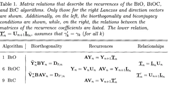
2.2. Matrix relations

The matrix relations (2.9)-(2.11) can be considered as a shorthand notation for the BlO algorithm: the relations (2.10) describe the recurrences for yn

286 M . H . GUTKNECHT

and yn, while (2.9) and (2.11) summarize the formulae for determining the

elements of TV, TV, and D,$;,,. These matrix relations hold as well after

n < v steps, and in fact are obtained for such an intermediate stage by

considering submatrices of the appropriate size.

Equation (2.10) can be simplified by introducing the (n + l ) x n leading principal submatrices of TV and TV, the extended tridiagonal matrices5

I T To a i Pi 7i "2 '•• Pn-2 7n-2 «n-l 7n-l

and the analogous matrices with tildes. Then we have altogether A Yn = Yn + 1Tn, A*Yn = Yn + 1Tn (n < «/), = D6 ; n, Y^BAY^ = BS;nTn (n<v), Dg ; nTn = T*nT>6,n (n<u). (2.23) (2.24) (2.25)

The first relation in (2.23) means that T

is the representation in the basis

{yo> • • •> Yn} of the restriction of A to the subspace K.

, which is mapped into

K-

\. The subspace K

is 'nearly invariant' as its image requires only one

additional space dimension. When it turns out that the component of Ay

_i

in this direction is relatively short, then we can expect that the eigenvalues

of T

are close approximations of eigenvalues of A. This is vaguely the

reasoning for applying the BlO algorithm to eigenvalue computations. There

are several reasons that make this argument dangerous. First, the basis is

not orthogonal, and thus T

is linked to A by an oblique projection only:

while in the Hermitian case the eigenvalues of T

are Ritz values, that is,

Galerkin or Rayleigh-Ritz approximations, they are in the non-Hermitian

case only Petrov-Galerkin approximations, which are sometimes referred to

as Petrov values. Second, since neither A nor T

are Hermitian in the case

considered here, eigenvalues need not behave nicely under perturbation.

A notorious problem with the Lanczos process is that in finite precision

arithmetic round-off affects it strongly. In particular, since only two

or-thogonality conditions are enforced at every step, while oror-thogonality with

respect to earlier vectors is inherited, a loss of (bi)orthogonality is noticed

5

By underlining Tn we want to indicate that we augment this matrix by an additional

row. We suggest reading Tn as 'T sub n extended'. The same notation will be used on

in practice, which means that T)s-,n is not diagonal. This is also a serious problem in the Hermitian case; we will return to it briefly in Section 18.

2.3. Normalization; simplification due to symmetry

As discussed before, in the BlO algorithm (Algorithm 1) the coefficients an, an, 0n-\, j3n-i, 7n, 7n, and 6n+\ are defined uniquely except that in (2.21i)

we are free to choose two of the three quantities 7n, 7n, and <5n+i. Special

versions of the algorithm are found by making a particular choice for two of the coefficients 7n, %, and 6n+i, and capitalizing upon the particular

choice. The classical choices for theoretical work are 7n := 7n := 1 (Lanczos

1950, Lanczos 1952, Rutishauser 1953, Householder 1964) or 7n = 7n and

<5n+1 ;= 1. The latter makes the two vector sequences biorthonormal and

yields (3n-\ = 7n- i ; that is, Tu = T j is real or complex symmetric, cf.

(2.18). (Consequently, (2.16) and (2.17) then coincide.) For numerical com-putations the former choice is risky with respect to overflow, and the latter is inappropriate for real nonsymmetric matrices since it may lead to some complex 7n. Therefore, in the real nonsymmetric case, the two choices

In •= In '•= y |<Stemp| ' <Wl :== ^temp/(inln) = <5temp/|<Stemp|, (2.26)

In •= ||ytemp|| , In •= ||ytemp|| , <Wl : = <5temp/'(7n7n), (2-27)

are normally suggested, but there may be a special reason for yet another one. Note that (2.27) requires two additional inner products. These are often justified anyway by the necessity of stability and round-off error control; see

Section 18.

Replacing, say, ")n = 1 (for all n) by some other choice means replacing Yn by

9n •= y n / rn, where rn := 7071 • • • 7n_i, (2.28)

which in view of (2.23) amounts to replacing Tn by

Tn := DfJ.TnDrjn, where Dr ; n := diag(r0, I \ , . . . , rn_x) , (2.29)

If 7n and 7n are chosen independently of ytemp and ytemP) the formulae

(2.21e)-(2.21j) can be simplified; cf. Algorithm 2 below.

If A and B are Hermitian and B is positive definite, starting with yo = yo and making the natural choice 7n := 7n and 6n > 0 leads to TV = Tu = Tu

(that is, Tj/ = Tj, is real) and yn = Yn (for all n). Thus, the recursion (2.21f) for yn is redundant, the costs are reduced to roughly half, and the

Lanczos vectors are orthogonal to each other. Moreover, one can choose 7n > 0 (for all n), which then implies that (5n-\ > 0 also. Finally, choosing 6n := <50 (for all n) makes Tu real symmetric. Then the BlO algorithm

becomes the symmetric Lanczos algorithm, which is often just called the

288 M. H. GUTKNECHT

If A is complex symmetric and yo = yo, then yn = yn (for all n). Again,

the costs reduce to about half. Now, setting 6n := 1 (for all n) makes Tu

complex symmetric, but this can be achieved in general and has nothing to do with A being complex symmetric. See Freund (1992) for further details on this case.

In Section 6 we will discuss yet other cases where the BlO algorithm simplifies.

3. Termination, breakdowns and convergence

The BlO algorithm stops with u := n + 1 when 6temp — 0, since atn+i would

become infinite or indefinite. We call v here the index of first breakdown

or termination. Of course, v is bounded by the maximum dimension of the

Krylov spaces, but u may be smaller for several reasons. The maximum dimension of the subspaces Kn denned by (2.1) depends not only on A but

also on yo; it is called the grade of yo with respect to A and is here denoted by z/(yo, A). As is easy to prove, it satisfies

y(yo, A) = min {n : dim/Cn = d i m £n +i } ,

and it is at most equal to the degree u( A) of the minimum polynomial of A. Clearly, the Lanczos process stops with ytemp = ytemp = o when v = u(A).

If this full termination due to ytemP = ytemp = o happens before the degree

of the minimum polynomial is reached, that is, if v < v(A), we call it an

early full termination. However, the BlO algorithm can also stop with either

ytemp = o or yt e m p = o, and even with (yt e m p, ytemP)B = 0 when yt e m p ^ o

and ytemp 7^ o. Then we say that it breaks down, or, more exactly, that we

have a one-sided termination or a serious breakdown, respectively6.

Lanczos (1950, 1952) was already aware of these various breakdowns. They have since been discussed by many authors; see, in particular, Fad-deev and FadFad-deeva (1964), Gutknecht (1990), Householder (1964), Joubert (1992), Parlett (1992), Parlett et al. (1985), Rutishauser (1953), Saad (1982), and Taylor (1982).

Of course, in floating-point arithmetic, a near-breakdown passed without taking special measures may lead to stability problems. Therefore, in prac-tice, breakdown conditions ' = o' and ' = 0' have to be replaced by other conditions that should not depend on scaling and should prevent us from numerical instability. We will return to this question in Section 19.

6

Parlett (1992) refers to a benign breakdown when we have either an early full termination or a one-sided termination.

3.1. Full termination

In the case of full termination, that is, when the BlO algorithm terminates with

ytemp = Ytemp = O, (3.1)

we can conclude from (2.10) that

AY,, = YVTV, ATYV = Yv%. (3.2)

This means that Ku and Kv are invariant subspaces of dimension v of A

and A*, respectively. The set of eigenvalues of TV is then a subset of the spectrum of A.

The formula AY,, = Y^T^ points to an often cited objective of the BlO algorithm: the similarity reduction of a given matrix A to a tridiagonal matrix TV. For the latter the computation of the eigenvalues is much less costly, in particular in the Hermitian case. However, unless v = N or the Lanczos process is restarted (possibly several times) with some new pair yV, y,, satisfying (2.4), it can never determine the geometric multiplicity of an eigenvalue, since it can at best find the factors of the minimal polynomial of A. In theory, to find the whole spectrum, we could continue the algorithm after a full termination with v < N by constructing first a new pair (y,,, yV) of nonzero vectors that are biorthogonal to the pair of vector sequences constructed so far, i.e., satisfy (2.4); see, for instance, Householder (1964), Lanczos (1950), Lanczos (1952), and Rutishauser (1953). Starting from a trial pair (y,y) one would have to construct

yk(yk,y)B/6k, (3.3a)

k=0 v-l

yu ••= y - X ) yf c( yf c' y )B* / ^ ' (3-3 b)

fc=0

and hope that the two resulting vectors are nonzero. Then, one can set 7^_i := /?„_! := 0, so that after the restart the relations (2.10) hold even beyond this v. If no breakdown or one-sided termination later occurs, and if any further early full termination is also followed by such a restart, then in theory the algorithm must terminate with ytemP = ytemp — o and v =

N. The relations (3.2) then hold with all the matrices being square of

order N. The tridiagonal matrix TJV may have some elements 7fc = Ac = 0 duetto the restarts, and the same will then happen to TV. Since Y^ and Y;v are nonsingular, Tjv is similar to A, and TJV is similar to A*. Unfortunately, in practice this all works only for very small N: first, as is seen from (3.3a)-(3.3b), the restart with persisting biorthogonality (2.2) requires all previously computed vectors of the two sequences, but these are

290 M. H. GUTKNECHT

normally not stored; second, completely avoiding loss of (bi)orthogonality during the iteration would require full reorthogonalization with respect to previous Lanczos vectors, which means giving up the greatest advantages of the Lanczos process, the short recurrences.

For the same reasons, finding all the roots of the minimal polynomial with the Lanczos process is in practice normally beyond reach: due to loss of (bi)orthogonality or because i>(A) is too large and the process has to be stopped early, only few of the eigenvalues are found with acceptable accuracy; fortunately, these are often those that are of prime interest.

3.2. One-sided termination

When the BlO algorithm stops due to

either yt e m p = o or yt e m p = o

(but not ytemp = ytemp = o), we call this a one-sided termination. In some

applications this is welcome, but in others it may still be a serious difficulty. In view of (2.10), it means that either K,u or £ „ is an invariant subspace of

dimension v of A or A*, respectively. For eigenvalue computations, this is very useful information, although sometimes one may need to continue the algorithm with a pair (yi,,yv) that is biorthogonal to the pairs constructed so far, in order to find further eigenvalues. Determining the missing vector of this pair will again require the expensive orthogonalization of a trial vector with respect to a z^-dimensional Krylov subspace, that is, either (3.3a) or (3.3b).

In contrast, when we have to solve a linear system, then ytemp = o is

all we aim at, as we will see in the next section. Unfortunately, when ytemp = o but ytemp 7^ °> we have a nasty situation where we have to find a

replacement for ytemP that is orthogonal to Kv. In practice, codes either just

use some ytemp that consists of scaled up round-off errors or restart the BlO algorithm. In either case the convergence slows down. The best precaution against this type of breakdown seems to be choosing as left initial vector yo a random one.

3.3. Serious breakdowns

Let us now discuss the serious breakdowns of the BlO algorithm, which we also call Lanczos breakdowns to distinguish them from a second type of serious breakdown that can occur additionally in the standard form of the biconjugate gradient method. Hence, assume that the BlO algorithm stops due to

In the past, the recommendation was to restart the algorithm from scratch. Nowadays one should implement what is called look-ahead. It is the curing of these breakdowns and the corresponding near-breakdowns that is ad-dressed by the look-ahead Lanczos algorithms which have attracted so much attention recently. We will discuss the look-ahead BlO algorithm and some of the related theory in Section 19, where we will also give detailed refer-ences. In most cases, look-ahead is successful. Oversimplifying matters, we can say that curing a serious breakdown with look-ahead requires that

(yv, A.kyv)-Q ^ 0 for some k, while the breakdown is incurable when

(y«,,A*y./>B = 0 (for all k > 0).

In theory, the condition (yv, Afcy^)B ^ 0 has to be replaced by a positive lower bound for the smallest singular value of a k x k matrix, but in practice even this condition is not safe.

The serious breakdown does not occur if A and B are Hermitian, B is positive definite, yo = yo> 7« = 7^, and 6n > 0 (for all n), since then Yn — yn (for all n), and (., .)B is an inner product. Also, choosing jn, 7n,

or 6n differently will not destroy this property. On the other hand, serious

breakdowns can still occur for a real symmetric matrix A if yo 7^ yo-Under the standard assumption B = I it was shown by Rutishauser (1953) (for another proof see Householder (1964)) that there exist yo and yo such that neither a serious breakdown nor a premature termination occurs; that is, such that the process does not end before the degree of the minimal polynomial is attained. Unfortunately, such a pair (yo, yo) is in general not known. Joubert (1992) even showed that, in a probabilistic sense, nearly all pairs have this property; that is, the assumption of having neither a prema-ture termination nor a breakdown is a generic property. This is no longer true if the matrix is real and one restricts the initial vectors by requiring y0 = y0 £ M.N. Joubert gives an example where serious breakdowns then

occur for almost all yo. Of course, the set of pairs (yo,yo) that lead to a breakdown never has measure zero. But practice shows that near-breakdowns that have a devastating effect on the process are fairly rare.

3.4- Convergence

Although in theory the BlO algorithm either terminates or breaks down in at most min{z/(yo, A), i>(yo, A*)} steps, this rarely happens in practice, and the process can be continued far beyond N. For small matrices this is sometimes necessary when one wants to find all eigenvalues or to solve a linear system. But the BlO algorithm is usually applied to very large matrices and stopped at some n < N, so that only (2.10) and (2.11) hold, but not (3.2). The

n eigenvalues of Tn are then considered as approximations of n eigenvalues

292 M. H. GUTKNECHT

border of the spectrum. For eigenvalues of small absolute value, the absolute error is comparable to the one for large eigenvalues; hence, the relative error tends to be large. Therefore, the method is best at finding the dominant eigenvalues. Lanczos (1950, p. 270) found a heuristic explanation for this important phenomenon. Some remarks and references on the convergence of Lanczos-type solvers will be made in the next section when we discuss the basic properties of the BlCG method.

An additional difficulty is that due to the loss of biorthogonality, eigenval-ues of A may reappear in Tn with too high multiplicity. One refers to these

extra eigenvalues as ghost eigenvalues. We will come back to this problem in Section 18.

4. The B I O R E S form of the BlCG method

Let us now turn to applying the Lanczos BlO algorithm to the problem of solving linear systems of equations A x = b . We first review the basic properties of the conjugate gradient (CG) and the conjugate residual (CR) methods and then describe a first version, B I O R E S , of the biconjugate gradi-ent (BlCG) method. In the next section we will further cover the M I N R E S

algorithm for the CR method and a first version of the QMR method. We assume that A is nonsingular and denote the solution of A x = b by xe x, its initial approximation by xo, the nth approximation (or iterate) by

xn, and the corresponding residual by rn := b — A xn. Additionally, we let

yo := ro, or yo := ro/||ro|| if we aim for normalized Lanczos vectors. As in (2.1), K,n is the nth Krylov space generated by A from yo, which now has

the direction of the initial residual. From time to time we also refer to the nth error, xex — xn. Note that rn = A(xe x — xn) .

4-1. The conjugate gradient and conjugate residual methods

We first assume that A and B are commuting Hermitian positive definite matrices and recall some facts about the conjugate gradient (CG) method of Hestenes and Stiefel (1952). It is characterized by the property that the nth iterate xn minimizes the quadratic function

x (-> ((xex - x), A(xe x - x ) )B

among all x £ xo + K.n. The standard case is again B = I. By

differenti-ation one readily verifies that the minimizdifferenti-ation problem is equivalent to the

Galerkin condition

(y,rn)B = 0 (for all y € Kn), i.e., Kn _LB rn. (4.1)

Note that

In view of (4.1) and (4.2), rn spans the orthogonal complement of fCn in

/Cn+i. Hence, if we let yo := ro and generate the basis {yfc}£_0 of JCn+\ by

recursively orthogonalizing A ym with respect to /Cm+i (m = 0 , . . . , n — 1),

then yn is proportional to rn, and by suitable normalization we can achieve

y« = rn. This recursive orthogonalization procedure is none other than the

symmetric Lanczos process, that is, the BlO algorithm with yo = yo and commuting Hermitian matrices A and B. Note also that by (4.2), rn =

pn(A)yo, where pn is a polynomial of exact degree n satisfying pn(0) = 1.

This property, which is equivalent to xn € xo + ICn, means that CG is a

Krylov space solver, as defined by (1.1). Of course, up to normalization, the residual polynomial pn is here the Lanczos polynomial of (2.3).

The directions xn—xn_i can be seen to be conjugate to each other (i.e.,

A-orthogonal with respect to the B-inner product, or, simply, AB-A-orthogonal), whence CG is a special conjugate direction method. In their classical CG method Hestenes and Stiefel (1952) chose B = I and thus minimized x i—> ((xex — x), A(xex — x)), which is the square of the A-norm of the error. (This

is a norm since A is Hermitian positive definite.) With respect to the inner product induced by A, we then have from (4.1) and (4.2)

K,n J-A (Xex ~ X«)> (X*x - Xn) ~ (Xex ~ X0) £ Kn.

This means that xo — xn = (xex — xn) — (xex — xo) is the A-orthogonal

projection of the initial error xex — xo into /Cn, and the error xex — xn is

the difference between the initial error and its projection. Therefore, the CG method can also be viewed as an orthogonal projection method in the error space endowed with the A-norm. Moreover, it can be understood as an orthogonal projection method in the residual space endowed with the A~1-norm.

If B = A = A* instead, we have

( ( xe x- x ) , A ( xe x- x ) )B = | | A ( xe x- x ) | |2 = | | b - A x | |2, (4-3)

which shows that the residual norm is now minimized. The B-orthogonality of the residuals means here that they are conjugate. The method is therefore called conjugate residual (CR) or minimum residual method. Normally, the abbreviation M I N R E S stands for a particular algorithm due to Paige and Saunders (1975) for this method. We will come back to it in Section 5. Like some other versions of the CR method, M I N R E S is also applicable to Hermitian indefinite systems; see Ashby, Manteuffel and Saylor (1990), Fletcher (1976).

Prom (4.1) and (4.2) we can conclude here that rn is chosen so that it is

orthogonal to A/Cn and ro — rn lies in AK-n. In other words, with respect

to the standard inner product in Euclidean space, ro — rn is the orthogonal

projection of ro onto A/Cn. Therefore, the CR method is an orthogonal

294 M. H. GUTKNECHT

Prom the fact that the CG-residuals are mutually orthogonal and the CR-residuals are mutually conjugate, it follows in particular that in both cases r,, = o for some v < N, and thus xu = xex- However, in practice

this finite termination property is fairly irrelevant, as it is severely spoiled by round-off.

So far we only know how to construct the residuals, but we still need an-other recurrence for the iterates xn themselves. As we will see in a moment,

such a recurrence is found by multiplying by A "1 the one for the residuals, that is, the one for the appropriately scaled right Lanczos vectors. This then leads to the three-term version7, ORES, of the conjugate gradient method (Hestenes 1951). The standard version of the CG method, OMlN, instead uses coupled two-term recurrences also involving the direction vectors, which are multiples of the corrections xn +i — xn. In the rest of this section and in

Section 8 we want to describe generalizations to the nonsymmetric case.

4-2. Basic properties of the BiCG method

If A is non-Hermitian, the construction of an orthogonal basis {yn} of

the Krylov space becomes expensive and memory-intensive, since the re-currences for yn generally involve all previous vectors (as first assumed in

(2.7)). Therefore, the resulting Arnoldi or full orthogonalization method (FOM) (Arnoldi 1951, Saad 1981) has to be either restarted periodically or truncated, which means that some of the information that was built up is lost. The same applies to the generalized conjugate residual (GCR) method (Eisenstat, Elman and Schultz 1983) and its special form, the G M R E S al-gorithm of Saad and Schultz (1986), which extends the M I N R B S algorithm to the nonsymmetric case.

However, we know how to construct efficiently a pair of biorthogonal se-quences { yn} , {yn}, namely by the BlO algorithm of Section 2. By requiring

that iterates xn € Xo + K.n satisfy the Petrov-Galerkin condition

( y , rn)B = 0 (for all y <E ICn), i.e., K,n _LB rn, (4.4)

we find the biconjugate gradient (BiCG) method. In contrast to the Galerkin condition (4.1) of the CG method, this one does not belong to a minimiza-tion problem in a fixed norm8.

7

The acronyms O R E S , OMIN, and ODiR were introduced in Ashby et al. (1990) as abbreviations for ORTHORES, ORTHOMIN, and ORTHODIR. We suggest using the short form whenever the basic recurrences of the method are short. Note that our acronyms

B I O R E S , BIOMIN, and B I O D I R for the various forms of the BiCG method fit into this pattern, as these algorithms also feature short recurrences.

8

Baxth and ManteufFel (1994) showed that BiCG and QMR fit into the framework of variable metric methods: in exact arithmetic, if the methods do not break down or terminate with v < N, then the iterates that have been created minimize the error in a

Now rn is chosen so that it is orthogonal to JCn and so that ro — rn lies

in A/Cn. This means that ro — rn is the projection of ro onto A/Cn along a

direction that is orthogonal to another space, namely /Cn, and, hence, is in

general oblique with respect to the projection space AK.n. Therefore, the

BiCG method is said to be an oblique projection method (Saad 1982, Saad 1996).

Since both the residual rn and the right Lanczos vector yn satisfy (4.4) and

both lie in K,n+\, and since we have seen in Section 2 that yn is determined up

to a scalar factor by these conditions, we can again conclude that the residual must be a scalar multiple of the Lanczos vector and that by appropriate normalization of the latter we could attain rn = yn.

The most straightforward way of taking into account the two conditions xn € xo + Kn and K,n J_B rn is the following one. Representing xn — xo in

terms of the Lanczos vectors we can write

xn = x0 + Ynkn, rn = r0 - A Ynkn, (4.5)

with some coordinate vector kn. Using A Yn = Yn +i Tn, see (2.23), and

with §! := [ 1 0 0 ••• ]T e Kn + 1 and p0 := ||ro|| (assuming ||yo|| = 1

here), we find that

rn = Yn +i (elPo - Tnkn) . (4.6)

In view of Y*BYn+i = [ D,5;n | o ], the Petrov-Galerkin condition (4.4),

which may be written as Y * B rn = o, finally yields the square tridiagonal

linear system

Tnkn = eipo, (4.7)

where now ei € Mn. By solving it for kn and inserting the solution into (4.5)

we could compute xn. However, this approach, which is sometimes called the

Lanczos method for solving linear systems, is very memory-intensive, as one has to store all right Lanczos vectors for evaluating (4.5). Fortunately, there are more efficient versions of the BiCG method that generate not only the residuals (essentially the right Lanczos vectors) but also the iterates with short recurrences. We could try to find such recurrences from the above relations, but we will derive them in a more general and more elegant way. Unless one encounters a serious breakdown, the BiCG method terminates theoretically with vv = o or yv = o for some v. Therefore, the BiCG

method also has the finite termination property, except that it is spoiled not only by round-off but also by the possibility of a breakdown (a serious

norm that depends on the created basis, that is, on A and yo- This result also follows easily from one of Hochbruck and Lubich (1997a)

296 M. H. GUTKNECHT

one or a left-sided termination). We must emphasize again, however, that it is misleading to motivate the CG method or the BiCG method (in any of their forms) by this finite termination property, because this property is irrelevant when large linear systems are solved. What really counts are certain approximation properties that make the residuals (and errors) of the iterates xn decrease rapidly. There is a simple, standard error bound that

implies at least linear convergence for the CG and CR methods (see, for instance, Kaniel (1966), Saad (1980, 1994, 1996)), but in practice superlinear convergence is observed; there are indeed more sophisticated estimates that explain the superlinearity under certain assumptions on the spectrum (van der Sluis and van der Vorst 1986, 1987, Strakos 1991, van der Sluis 1992, Hanke 1997). These bounds are no longer valid in the nonsymmetric case, but some of the considerations can be extended to it (van der Vorst and Vuik 1993, Ye 1991). The true mechanism of convergence lies deeper, and seems to remain the same in the nonsymmetric case. For the CR method and its generalization to nonsymmetric systems it has been analysed by Nevanlinna (1993). For the BiCG method convergence seems harder to analyse, however. Recently, a unified approach to error bounds for BiCG, QMR, FOM, and G M R E S , as well as comparisons among their residual norms, have been established in Hochbruck and Lubich (1997a).

The BiCG method is based on Lanczos (1952) and Fletcher (1976), but, as we will see, there are various algorithms that realize it.

4-3. Recurrences for the BiCG iterates; the consistency condition

The recurrence for the iterates xn is obtained from the one for the

re-siduals by following a general rule that we will use over and over again. By definition, xn — xo € fCn for any Krylov space solver, and thus (4.2)

holds; here Kn is still the nth Krylov space generated by A from yo =

To-Since rn = pn(A)yo with a polynomial pn of exact degree n, the vectors

ro, • • •, rn_ i span Kn (even when they are linearly dependent, in which case JCn = JCn-i). Therefore, if we let

Rn := [ ro ri • • • rn_ i ], Xn := [ xo xi • • • xn_i ],

and define the extended (n + 1) x n Frobenius (or companion) matrix - 1 - 1 ••• - 1

1

¥„:=

1 then we have, in view of xn — Xo £ /Cn,

with some upper triangular n x n matrix \J

and an extra minus sign. Each

column sum in F

is zero, that is, [ 1 1 • • • 1 ] F

= o

, and therefore,

for an arbitrary b G C^, multiplication of F

from the left by the N x (ra+1)

matrix [ b b • • • b ] yields an N x n zero matrix. Therefore,

I W i F

= ([ b • • • b ] - AX

) F

= - A X

F

= A R ^ . (4.9)

Since r

and Ar

_i are both represented by polynomials of exact degree

m, the diagonal elements of \J

cannot vanish. Hence, if we let

H

:= Hn\J

,

we can write (4.8) and (4.9) as

Rn = - X

H

A R , = Hn

m

, (4-10)

where H

is an (n + 1) x n upper Hessenberg matrix that satisfies

e

H

= o

, where e

:=[ 1 1 ••• 1 ] , (4.11)

as a consequence of e

F

= o

. This is the matrix form of the consistency

condition for Krylov space solvers. It means that in each column of H^

the elements must sum up to 0; see, for instance, Gutknecht (19896). This

property is inherited from F

. The relations in (4.10) are the matrix

rep-resentations of the recurrences for computing the iterates and the residuals:

x

is a linear combination of r

_i and xo,..., x

_i, and r

is a linear

com-bination of Ar

_i and r o , . . . , r

_i. Note that the recurrence coefficients,

which are stored in H

, are the same in both formulae.

Another, equivalent form of the consistency condition is the property

p

{0) = 1 of the residual polynomials.

We call a Krylov space solver consistent if it generates a basis consisting

of the residuals (and not of some multiples of them).

4-4- The

algorithm

In the usual, consistent forms of the BiCG method, the Lanczos vectors y

are equal to the residuals r

and thus the Lanczos polynomials satisfy the

consistency condition p

(0) = 1. To apply the above approach, we have to

set H

:= T

and Rn := Y

. Therefore, the zero column sum condition

requires us to choose j

:= — a

— fl

-\. However, this can lead to yet

another type of breakdown, namely when a

+ P

-i = 0. Following Bank

and Chan (1993) we call this a pivot breakdown (for reasons we will describe

later, in Section 9), while a breakdown due to 6

= 0 in the BlO algorithm

is referred to as a Lanczos breakdown

, as before.

9 _{The dimension of the vectors o and e is always defined by the context.}

10 _{In Gutknecht (1990) we suggested calling a pivot breakdown a normalization breakdown,}

298 M. H. GUTKNECHT

Recalling that the formulae for the BiO algorithm can be simplified if j n

is independent of Stemp, and adding the appropriate recurrence for the

ap-proximants xn, we find the following BlORES version of the BlCG method. ALGORITHM 2. ( B I O R E S FORM O F THE B I C G METHOD)

For solving A x = b , choose an initial approximation Xo, set yo := b — Axo, and choose yo such that 60 := (yo,yo)B 7^ 0- Then apply Algorithm 1 (BiO) with

7n := -an - /?„_! (4.12)

and some 7n 7^ 0, so that (2.21e)-(2.21j) simplify to

yn +i := (Ayn - ynan - yn-iPn-i)/ln, (4.13a)

yn+i := (A^yn-ynan-yn-i0n-i)/%, (4.13b)

6n+i := (yn+i,yn+i)B- (4.13c)

Additionally, compute the vectors

xn +i := - ( yn + xnan + xn_i/?n_i)/7n. (4.13d)

If j n = 0, the algorithm breaks down ('pivot breakdown'), and we set v :— n.

If yn+i = o, it terminates and xn+i is the solution; if yn+i ^ o, but

<5n+i = 0, the algorithm also breaks down ('Lanczos breakdown' if yn+i 7^ o,

'left termination' if yn+i = o). In these two cases we set v := n + 1.

First we verify the relation between residuals and iterates.

L e m m a 4.1 In Algorithm 2 ( B I O R E S ) the vector yn is the residual of the

nth iterate xn; that is, b — A xn = yn (n = 0 , 1 , . . . , v).

Proof. First, b —Axo = yo by definition of yo- Assuming n > 1, b—Axn =

yn, and b — Axre_! = yn_ i , and using (4.13a)-(4.13d), (2.21e), (2.21j), and

(4.12), we get

b - Axn +i = b + (Ayn

= b + (Ayn - ynan - yn-iPn-i + b(an + f3n-\))hn

which is what is needed for the induction. When n = 0, the same relations hold without the terms involving /3_i. •

solvers. Joubert (1992) calls the pivot breakdown a hard breakdown since it causes all three standard versions of the BiCG method discussed in Jea and Young (1983) to break down, as we will see in Section 9. In his terminology the Lanczos breakdown is a soft breakdown. Brezinski, Redivo Zaglia and Sadok (1993) use the terms true breakdown and ghost breakdown, respectively, while Freund and Nachtigal (1991) refer

to breakdowns of the second kind and breakdowns of the first kind. However, we will see

that in the algorithms most often used in practice, it is easier to circumvent a pivot (or hard, or true, or second kind) breakdown than a Lanczos breakdown.