Sunset time and the economic effects of social jetlag:
evidence from US time zone borders
Postprint (Author accepted manuscript)
Published online 2019-04-13
Giuntella, Osea; University of Pittsburgh, United States
Mazzonna, Fabrizio; Faculty of Economics, Università della Svizzera italiana, Switzerland
Journal of Health Economics
2019 / Vol. 65 / May / pp. 210-226
Published version:
https://doi.org/10.1016/j.jhealeco.2019.03.007
Published under a
CC BY-NC-ND 4.0
license
The rapid evolution into a 24 h society challenges individuals’ ability to conciliate work
schedules and biological needs. Epidemiological research suggests that social and
biological time are increasingly drifting apart (“social jetlag”). This study uses a spatial
regression discontinuity design to estimate the economic cost of the misalignment
between social and biological rhythms arising at the border of a time-zone in the presence
of relatively rigid social schedules (e.g., work and school schedules). Exploiting the
discontinuity in the timing of natural light at a time-zone boundary, we find that an extra
hour of natural light in the evening reduces sleep duration by an average of 19 minutes
and increases the likelihood of reporting insufficient sleep. Using data drawn from the
Centers for Disease Control and Prevention and the US Census, we find that the
discontinuity in the timing of natural light has significant effects on health outcomes
typically associated with circadian rhythms disruptions (e.g., obesity, diabetes,
cardiovascular diseases, and breast cancer) and economic performance (per capita
income). We provide a lower bound estimate of the health care costs and productivity
losses associated with these effects.
Accepted Manuscript
Title: Sunset Time and the Economic Effects of Social Jetlag Evidence from US Time Zone Borders
Author: Osea Giuntella Fabrizio Mazzonna
PII: S0167-6296(18)30971-8
DOI: https://doi.org/doi:10.1016/j.jhealeco.2019.03.007 Reference: JHE 2192
To appear in: Journal of Health Economics Received date: 22 October 2018
Revised date: 18 January 2019 Accepted date: 27 March 2019
Please cite this article as: Osea Giuntella, Fabrizio Mazzonna, Sunset Time and the Economic Effects of Social Jetlag Evidence from US Time Zone Borders, <![CDATA[Journal of Health Economics]]> (2019), https://doi.org/10.1016/j.jhealeco.2019.03.007
This is a PDF file of an unedited manuscript that has been accepted for publication. As a service to our customers we are providing this early version of the manuscript. The manuscript will undergo copyediting, typesetting, and review of the resulting proof before it is published in its final form. Please note that during the production process errors may be discovered which could affect the content, and all legal disclaimers that apply to the journal pertain.
Accepted Manuscript
Sunset Time and the Economic Effects of Social Jetlag
Evidence from US Time Zone Borders
Osea Giuntella∗ University of Pittsburgh
Fabrizio Mazzonna†
Universit´a della Svizzera Italiana (USI) Draft
March 26, 2019
Abstract
The rapid evolution into a 24h society challenges individuals’ ability to conciliate work schedules and biological needs. Epidemiological research suggests that social and biologi-cal time are increasingly drifting apart (“social jetlag”). This study uses a spatial regression discontinuity design to estimate the economic cost of the misalignment between social and biological rhythms arising at the border of a time-zone in the presence of relatively rigid social schedules (e.g., work and school schedules). Exploiting the discontinuity in the timing of nat-ural light at a time-zone boundary, we find that an extra hour of natnat-ural light in the evening reduces sleep duration by an average of 19 minutes and increases the likelihood of reporting insufficient sleep. Using data drawn from the Centers for Disease Control and Prevention and the US Census, we find that the discontinuity in the timing of natural light has signifi-cant effects on health outcomes typically associated with circadian rhythms disruptions (e.g., obesity, diabetes, cardiovascular diseases, and breast cancer) and economic performance (per capita income). We provide a lower bound estimate of the health care costs and productivity losses associated with these effects.
Keywords: Time Allocation, Health, Work Schedules, Regression Discontinuity
JEL Classification: J22; I12; C31
∗University of Pittsburgh. 230 S Bouquet St, Pittsburgh, PA 15260. Email: [email protected].
†Universit´a della Svizzera Italiana (USI). Department of Economics, via Buffi 13, CH-6904, Lugano. Email:
[email protected]. We are thankful to Timothy Bond, Daniel Berkowitz, Amithab Chandra, John Cawley, Martin Gaynor, Matthew Gibson, Daniel Hamermesh, Kevin Lang, Anita Mucherjee, Andrew Oswald, Raphael Parchet, Daniele Paserman, Franco Peracchi, Climent Quintana-Domeque, and Noam Yuchtman, for their comments and sug-gestions. We are also grateful to participants at workshops and seminars at the CEPRA/NBER Workshop, ETH Zurich, Hamburg University, University of Lausanne, University of Lucerne, the Max Planck Institute (Rostock), University of Munich, Universidad de Navarra, University of Oxford, University of Pittsburgh, Universitat Pompeu Fabra, Research Institute for the Evaluation of Public Policies (IRVAPP) Stockholm School of Economics, University of Surrey, Uni-versity of Warwick, West Virginia UniUni-versity, the Society of Labor Economists Meetings, the Population Association of America Meetings, American Society of Health Economists Conference, V Health Econometrics Workshop, the IX Workshop on the Economics of Risky Behaviors.
Accepted Manuscript
1
Introduction
There is increased concern that the rapid evolution into a 24-hours society led to a mis-alignment of social and biological rhythms, with detrimental consequences for overall health
(Rajaratnam and Arendt,2001). Social schedules can conflict with individual circadian rhythms,
the physiological processes (physical, mental and behavioral) characterized by a 24-hour cycle affecting sleep-wake-cycles and other physiological functions (e.g., hormone release, body tem-perature). Chronobiologists refer to the discrepancy arising between biological and social time as “social jetlag” (Roenneberg et al.,2012). The goal of this paper is to analyze the causal effects of social jetlag on health and economic outcomes exploiting the quasi-experiment provided by the variation in the timing of natural light introduced by time zone borders.
The allocation of time between work, home-production, leisure and rest has been a central question in the economic literature (Becker,1965;Gronau,1977;Aguiar and Hurst,2007;Aguiar
et al.,2013). Working schedules, school start times, and generally the organization of social time
are subject to growing economic incentives for coordination and synchronization (Weiss, 1996;
Stein and Daude,2007;Hamermesh et al.,2008). However, the “forced synchornization” of
sched-ules can disrupt human circadian rhythms and have detrimental effects on health and productiv-ity (Cappuccio et al.,2010). Economists have largely neglected the possible detrimental effects of “forced synchronization” of time-use on health and economic productivity (Mullainathan,2014). Motivated by the growing medical awareness on the undermining effects of circadian rhythms disruption, our goal is to assess how the forced synchronization imposed by time zones and the rigidity of social schedules affect health and economic performance.
As all mammals, humans respond to environmental light, the most important signal regulat-ing our biological clock. However, human beregulat-ings are the only animal species that deliberately tries to master nature, for instance depriving themselves of sleep. Individuals adjust their sched-ules responding to incentives to economic and social coordination. The inability to master the biological responses of our body gives rise to the health and human capital effects we estimate in this study. The timing of natural light is determined by the existence of time zones and has a direct effect on the sleep-wake cycle. The human body reacts to environmental light, producing more melatonin when it becomes darker.1 The misalignment of sleep and wake rhythms with the daily cycle of physiological processes desynchronizes the release of hormones such as mela-tonin, cortisol (“the stress hormone”), ghrelin (the “hunger hormone”) and leptin (the “satiety hormone”). As these hormones are related to stress, metabolism and inflammation, circadian rhythms disruptions can directly affect health by increasing the risk of metabolic and cardiovas-cular diseases, and cancer progression (Luyster et al.,2012). Medical studies provide evidence of
1There is voluminous scientific evidence on the relationship between environmental light and sleep timing (see
Roenneberg et al.,2007, for a review). Circadian rhythms are governed by the suprachiasmatic nucleus (SCN), or internal pacemaker also known as the body’s master clock. The SCN synchronizes biological rhythms with envi-ronmental light, a process known as “entrainment”. When there is less light, the SCN stimulates the production of melatonin, also known as “the hormone of darkness”, which in turn promotes sleep in diurnal animals, including humans.
Accepted Manuscript
important associations of exposure to artificial and natural light at night with sleep loss, weight gain, cognitive impairment and chronic diseases such as cardiovascular diseases, and diabetes(Shi et al.,2013;Schmidt et al.,2007). There is also observational evidence on shift workers and
experimental evidence on rats suggesting that circadian rhythms disruption increases the risk of certain types of cancer (Haus and Smolensky,2013; Blask et al.,2005). However, most of the evidence is based on descriptive studies or laboratory experiments. Observational studies do not shed light on the mechanisms underlying these associations, while laboratory experiments provide a limited understanding of the effects of circadian rhythms disruptions in the real-world
(Roenneberg,2013). Furthermore, they do not allow us to understand how individual behaviors
are affected by social constructs such as work schedules, school start times, and other forms of “forced synchronization”.
Our main contribution is to provide a causal estimate of the health and economic effects of social jetlag using non-experimental data. Time zones allow us to identify an exogenous variation in the timing of natural light. In counties lying on the eastern (right) side of a time zone boundary, sunset time occurs an hour later than in nearby counties on the opposite side of the boundary (see Figure1). More generally the onset of daylight is delayed by an hour. Henceforth, we will refer to these counties as counties on the late sunset side of the border. Because of the delayed onset of daylight and the biological link between environmental light and the production of melatonin throughout the day, individuals on the late sunset side of a time zone boundary will tend to go to bed at a later time. In addition, as prime-time evening shows air at 10 p.m. Eastern and Pacific, 9 p.m. Central and Mountain, TV programs may also affect bedtime and reduce or reinforce the effect of sunset time (Hamermesh et al., 2008). Note that if people were to compensate by waking up later, solar, and TV cues would have no effect on sleep duration. However, because of economic incentives, social schedules —such as working schedules, and school start times— tend to be rigid and unresponsive to solar cues. Thus, many individuals are not able to fully compensate in the morning by waking up at a later time.
Given the direct biological link between the dark-light and the sleep-wake cycle, sleep is our primary outcome of interest. Sleep is a commodity we all demand. Yet, statistics suggest many of us sleep less than the recommended 7-8 hours.2 A survey conducted in 2013 by the U.S. National Sleep Foundation found that Americans are more sleep-starved than their peers abroad, and the Institute of Medicine (2006) estimates that 50-70 million US adults have sleep or wakefulness disorder (Altevogt et al.,2006). Estimates suggest that in many countries, individuals are sleeping as much as two hours less per night than did their ancestors one hundred years ago and that the “unnatural” timing of sleep may be the “most prevalent high-risk behavior in modern society”
(Roenneberg, 2013). Biddle and Hamermesh (1990) were the first to formalize the analysis of
the sleeping decision and econometrically analyze its relationship with economic incentives.3
2See the recent sleep guidelines from the National Heart, Lung, and Blood Institute:http://www.cdc.gov/sleep/
about_sleep/how_much_sleep.html. For more anecdotal evidence on the current sleep crisis seeHuffington(2016).
3The discussion on the economics of sleeping began earlier in the 1970s with an article byEl Hodiri(1973),
Accepted Manuscript
Despite the large heterogeneity in sleep duration in the population and the growing medical evidence on the risks associated with short sleep duration and poor sleep quality, only recently economists have attempted to empirically analyze the economic causes and consequences of sleep deprivation.Using data from the American Time Use Survey (ATUS), we find that employed people living in counties on the late sunset side of the time zone border sleep on average 19 fewer minutes than employed people living in neighboring counties on the opposite side of the border because of the one-hour difference in sunset time. More generally, individuals on the late sunset side of a time zone boundary are more likely to be sleep deprived, more likely to sleep less than 6 hours, and less likely to sleep at least 8 hours. The effects are larger among individuals with early working schedules and among individuals with children of school age. These results are confirmed using an alternative metric of sleep deprivation drawn from the Behavioral Risk Factor and Surveillance Survey (BRFSS). Reassuringly the trend in sleep duration metrics across the border mirrors the linear (mechanical) trend in the timing of sunset across the time zone boundary. Using health information available at the county-level (source: Centers for Disease Prevention and Control, CDC), we also find evidence of significant discontinuities in the incidence of obesity, diabetes, cardiovascular diseases, and breast cancer. Summarizing these outcomes with a standardized composite health index, we find that living on the late sunset side of the border decreases the index by .3 standard deviations. These effects are the consequences of a long-term-exposure to circadian rhythms disruptions.
There are several biological channels through which the discontinuity in sunset time at the time-zone border may affect these health outcomes. First, the reduction in sleep duration has been associated with the release of hormones that are correlated with weight gain and with inflammations associated with cardiovascular diseases and certain types of cancer. The delay of natural light may also have direct effects on physical activity and on eating behaviors. In the Appendix, we exploit time use data to analyze the role of these alternative mechanisms. Our findings rule out the hypothesis that changes in physical activity may explain the observed discontinuities in health outcomes. However, we do find evidence that individuals exposed to more sunlight in the evening tend to eat later and are more likely to dine-out. These effects contribute to explaining the detrimental impact of social jetlag on obesity and, in turn, diabetes.
To gauge an idea about potential costs of circadian rhythms disruptions we provide a back of the envelope estimate of health care costs and productivity losses associated with the disconti-nuity in the sunlight onset occurring at the border of a time zone. We calculate that the circadian misalignment increases health care costs by at least 2 billion dollars. Productivity losses associ-ated with the insufficient sleep induced by the extra hour of light in the evening are equivalent to 4.40 million days of work.
Having shown that the delay of natural light onset has significant effects on health outcomes, we turn to the analysis of its possible effects on economic productivity. To this goal we test for formalize the analysis of the sleeping decision and econometrically analyze its relationship with economic incentives.
Accepted Manuscript
the presence of discontinuities in zip code-level income per capita as a measure of economic productivity. Using zip code level data from the 2010-2014 American Community Survey, we show that within commuting zones spanning across a time-zone boundary –where mobility costs should be low and arbitrage should eliminate any wage differential– there are not significant differences in income per capita across the border. However, as we exclude from the analysis counties in commuting zones spanning across the time zone boundary, we do find evidence that wages tend to be 3% lower on the late sunset side of the time zone border. These are long-run effects as they capture cross-sectional differences in the exposure to a delay in the onset of sunset time. Despite these differences, we find no evidence of residential sorting. In particular, there is no significant discontinuity in home values, rents, and commuting times. Nor we find evidence of discontinuity in population density at the time zone border. Persistent differences across commuting zones are consistent with recent evidence against the full mobility benchmark (Autor et al., 2013; Bartik, 2017; Amior and Manning, 2015). There are also other potential explanations for why individuals on the late sunset side of the border would not move or adjust their schedules. More light in the evening may have negative effects on health and income, but it may increase the marginal utility from leisure time generating a trade-off between health and leisure enjoyment. Finally, individuals may have inaccurate self-perceptions of their biological needs and may underestimate the detrimental effects of circadian rhythms disruption on health. Time inconsistency, bounded rationality, cognitive impediments, self-serving bias may explain individual sub-optimal behavior (Mani et al.,2013;Banerjee and Mullainathan,2008).Taken together, our findings highlight that while schedules’ synchronization may respond to economic incentives to coordination, the conflict arising between our biological and social schedule may result in non-negligible costs because of the negative effects of social jetlag on health and economic productivity.
Our results are robust to a large battery of robustness checks. First, we show that there are no discontinuities in our covariates and in predetermined characteristics known not to be affected by the treatment. Second, we find no significant relationship with outcomes that should not be affected by circadian rhythms disruption (e.g., cancer types that are mostly determined by genetic inheritance). Furthermore, our results are robust to the bandwidth choice, to the inclusion of state-fixed effects and the adoption of alternative estimation procedures that takes into account the methodological challenges that typically arise in a geographic RD design (Imbens and Zajonc,
2011).
This research contributes to a small but growing number of studies in the economic literature analyzing the health effects of sleep deprivation, and more generally, the effects of circadian rhythms disruptions. In a recent study,Jin et al.(2015) study the health effects of Daylight Saving Time (DST) and find that health slightly improves in the short run (4 days) when clocks are set back by one hour in Fall but no evidence of detrimental effects when moving from standard time to DST in Spring. Using a similar strategy, Smith(2016) shows that DST increases fatal crashes, whileDoleac and Sanders (2015) provide evidence of a 7% decrease in robberies following the
Accepted Manuscript
shift to DST, and the relative change in the timing of daylight. We differentiate from Jin et al.(2015), as rather than focusing on the short-run effects of the shift to DST, we examine the long-run effects of exposure to light in the evening on measures of health and chronic diseases that are less likely to vary in the short-run (e.g., obesity, diabetes etc.). Our paper is related to
Gibson and Shrader (2018) who use within-time zone variation in sunset time to identify the
effects of sleep on wages. They find that a one-hour increase in average daily sleep increases productivity to a greater extent than does a one-year increase in education. However, we take a different econometric approach exploiting the discontinuity at the time zone border rather than the variation in sunset time within a time zone border. We argue that this mitigates the concern that differences in sunset time within a time-zone may be correlated with unobservable determinants of health and human capital as counties in proximity of the border may be more similar to each other than counties on the two edges of the same timezone (e.g., coastal vs internal cities). Furthermore, we shed further light on the mechanisms of the reduced-form effect of exposure to later light in the evening on economic outcomes by focusing on a battery of health metrics that may have a direct impact on economic productivity and health care costs. Finally, this paper is also related to the studies analyzing the effects of school start times on academic achievement (Carrell et al.,2011;Edwards,2012;Dills and Hernandez-Julian,2008) and showing that even small differences in school start times can have large effects on academic outcomes. In particular, our design is similar toHeissel and Norris(2017) who use the time zone boundary in Florida to instrument for the hours of sunlight before school and show that moving start times one hour later relative to sunrise increases test scores. However, none of these papers exploits the sharp discontinuity at time zone borders to analyze the medium and long-run effects of circadian rhythms disruptions on health and economic outcomes.
This paper is organized as follows. In Section2, we briefly discuss the context. Section 3 de-scribes the data and our identification strategy. Section4discusses the main results documenting the discontinuities in sleep, health, and economic outcomes. Robustness checks are discussed in Section5. In the Appendix, we explore the potential mechanisms explaining the effects on health and productivity. Concluding remarks are provided in Section6.
2
Background: US Time Zones and Solar and TV Cues
2.1 US Time-zones
As shown in Figures 1, the United States are divided into 4 four main time zones (Eastern, Central, Mountain, and Pacific). The time zones were first introduced in the US in 1883 to regulate railroad traffic. However, even in relatively nearby areas, scheduling was far from being uniform at that time (Hamermesh et al.,2008; Winston et al.,2008). The four current U.S. time zones were officially established with the Standard Time Act of 1918, and there have only been some changes since then, primarily at their boundaries. The Eastern time zone was set -5 hours with respect to Greenwich Mean Time (GMT), and the other three time zones (Central, Mountain
Accepted Manuscript
and Pacific) differ from that by -1, -2, and -3 hours, respectively. It is worth noting that time zone borders do not always coincide with state borders. In 12 of the contiguous US states, different counties follow different time zones.Since 1918, a few counties petitioned the Department of Transportation for a change in their time zones (USNO 2015) especially in the years immediately after the time zones introduction. Almost all changes implied a westward movement of the three time zone boundaries, “reflecting the orientation of commerce eastward at that time” (Bartky and Harrison, 1979). Moreover, there are some small bordering counties that unofficially adopted a different time zone representing an exception to the federal law. Again most of these exceptions imply a westward movement of the time zone borders. While this suggests that time zone boundaries are at least partially endogenous, the westward movement of boundaries would have, if anything, negative effects in terms of our treatment of interest. Counties moving to the late sunset side of a time zone boundary would move from early sunset areas – where the conflict between natural light and social schedules is minimized– to late sunset areas – where the delay of natural light onset would induce a misalignment between biological and social daily rhythms. Moreover, our results are robust to the exclusion of counties that petitioned to relocate time zone boundaries (reported in the Appendix).
A few local labor markets and commuting zones span over two time zones. In the analysis, we show how the exclusion of these areas affects our main results. Furthermore, we provide several tests supporting the continuity assumption underlying our geographical regression discontinuity design.
2.2 Timing of Television Programs
The effect of the timing of natural light may be mediated by the different timing of TV programs across time zones. Television networks usually broadcast two separate feeds, namely the “eastern feed” that is aired at the same time in the Eastern and Central time zones and the “western feed” for the Pacific time zone. In the Mountain time zone, networks may broadcast a third feed on a one-hour delay from the Eastern time zone. Television schedules are typically posted in Eastern/Pacific time, and thus, programs are conventionally advertised as “tonight at 9:00/8:00 Central and Mountain”. Therefore, in the two middle time zones, television programs start nominally an hour earlier than in the Eastern and Pacific time zones. Prime time shows start nominally an hour later on the late sunset side of the time zone boundary between the Central and Eastern time zones, an hour earlier on the late sunset side of the time zone boundary between Mountain and Pacific, and at the same time along the counties bordering with the time zone border between Central and Mountain time zones.
Thus, we expect that if TV schedules affect individual bedtime, the discontinuity in bedtime should be larger along the Central–Eastern time zone border and smaller along the Pacific– Mountain time zone border. We examine the role of TV schedules in SectionCin the Appendix showing that television schedules do not play a major role in explaining the discontinuity in
Accepted Manuscript
sleep duration that we observe at the time zone border.3
Data and Identification Strategy
3.1 Data
Individual Time-Use Data (ATUS)
Our analysis of the discontinuity in sleep duration is largely based on data drawn from the American Time Use Survey (ATUS) conducted by the U.S. Bureau of Labor Statistics (BLS) since 2003. Our sample covers the years 2003–2013. The ATUS sample is drawn from the exiting sample of Current Population Survey (CPS) participants. The respondents are asked to complete a detailed time use diary of their previous day that includes information on time spent sleeping and eating. In 2003, 20,720 individuals participated in the survey. Since 2004, on average, more than 1,100 individuals have participated in the survey each month since 2004. This yields a total sample of approximately 148,000 individuals. In our analysis, we restrict attention to individuals in the labor force (both employed and unemployed)4 living within 250 miles of each time zone boundary (Pacific–Mountain, Mountain–Central, Central–Eastern). This is achieved by merging the ATUS individuals with CPS data to obtain information on the county of residence of ATUS respondents. Unfortunately, CPS does not release county information for individuals living in counties with fewer than 100,000 residents; thus, we can match only 44% of the sample. The results obtained using ATUS data are therefore representative of more urbanized and densely populated counties (see Figure2).5
We further restrict our sample to people aged 18 to 55 years to avoid the confounding effect of retirement and the selection issue that might arise focusing on high-school age workers.6 We also limit the analysis to individuals who sleep between 2 and 16 hours per night.7 After imposing these restrictions, the sample comprises 18,639 individuals, of whom 16,557 were employed. Note that in practice, when using the ATUS sample, we do not include Arkansas and Idaho as after imposing our sample restrictions we are left with no observations for these two states.
Employment status was determined on a series of questions relating to their activities during the preceding week. We also have information on whether the wake-up day was a workday for someone.
Our primary outcome of interest is sleep duration. We count only night sleeping by excluding naps (sleep starting and finishing between 7am and 7pm). However, the results are unchanged when including naps in the main variable (see Table A.1-A.2). We also consider alternative
4We exclude people not in the labor force because this category includes individuals disabled due to an illness
lasting at least 6 months.
5FigureA.2reports the time zone borders, state borders, and the major cities in the U.S..
6Our main results are substantially unchanged if we further restrict the sample to prime-age workers (25 to 55
years old).
7Those so excluded are mostly individuals who did not report any sleep. However, including those sleeping less
Accepted Manuscript
measures of sleep duration such as indicators for reported sleep of at least 8 hours (or less than 6), being asleep at midnight or being awake at 7.30am. These metrics are often used in sleep studies (Cappuccio et al.,2010). In our analysis, we include several socio-demographic controls, such as age, sex, education, race, marital status, nativity status, year of immigration, and number of children, that might affect individuals’ sleeping behavior. Table A.3in the Appendix reports summary statistics for the variables of interest. Note that approximately 50% of the ATUS sample is interviewed over the weekend, and thus the average sleep duration in the sample is longer than that observed during the workweek (see Figure A.1). It is worth noting that self-reported sleep tends to overestimate objective measures of sleep duration (Lauderdale et al.,2008).Basneret al. (2007) note that the values for sleep time may overestimate actual sleep because the ATUS
Activity Lexicon includes transition states (e.g., falling asleep).8
As mentioned above, an important limitation of the ATUS data is that we can only identify a limited set of counties (see Figure 2) because of the confidentiality restriction and because the survey does not cover all US counties. To test for the external validity of the results we integrate the analysis using alternative data sources. As an alternative metric for sleep deprivation we use data drawn from the Behavioral Risk Factor and Surveillance Survey which since 2008 contains a core question on the number of days that an individual felt sleep deprived over the previous months.9
The American Time Use Survey also contains information on BMI and self-reported health. Unfortunately, information on these health outcomes is not available in all survey years. Ques-tions on self-reported health status are only available since 2006, while information on body weight is available in the Eating Module included in the survey in the 2006-2009 waves. Us-ing ATUS data we analyze time zone discontinuities in overweight status (BMI> 25), obesity (BMI> 30), and the likelihood of reporting poor health status, defined as reporting poor or fair health status, as is common in the literature using metrics of self-reported health status. In Sec-tion5we address the potential concern related to the measurement error in the weight variables.
County and Zip Code Level Data
To overcome the limitations of the ATUS data, we integrate our analysis using county-level data from the Centers for Disease Prevention and Control (CDC). For obesity and diabetes, we use the CDC county diabetes and obesity prevalence estimates (2004-2013). Prevalence estimates are obtained using data from CDC’s Behavioral Risk Factor Surveillance System (BRFSS) and from the US Census Bureau’s Population Estimates Program. The county-level estimates for the over 3,200 counties or county equivalents (e.g., parish, borough, municipality) in the 50 US states, Puerto Rico, and the District of Columbia (DC) were based on indirect model-dependent
8While self-reported metrics of sleep are prone to measurement error, the fact that using different metrics of
sleep drawn from different surveys we obtain results tending in the same direction is reassuring and suggests that measurement error may not systematically vary across the time zone boundary.
9The exact question is: “During the past 30 days, for about how many days have you felt you did not get enough
Accepted Manuscript
estimates using Bayesian multilevel modeling techniques. These imputation techniques de facto reduce differences at the border of a time-zone as they smooth the data for counties with less observations and thus smoothing the discontinuities at the time zone border.10Data on cardiovascular diseases are drawn directly from the BRFSS (2007-2012). We calculated the share of individuals in the working age population (18–65) reporting any heart disease (e.g., acute myocardial infarction (AMI), coronary and angina disease, stroke). This information is available for approximately 70% of the US counties. These data are self-reported and thus do not include mortality data.
Cancer data are provided by the National Program of Cancer Registries Policy, Cancer Surveil-lance System (NPCR-CSS), CDC and by the National Cancer Institute’s SurveilSurveil-lance, Epidemiol-ogy, and End Results (SEER) Program. Population counts for denominators are based on Cen-sus populations as modified by the National Cancer Institute (NCI). Rates are calculated using SEER*Stat.11
For simplicity, in the main text we restrict the analysis to a composite health index which we constructed normalizing and summing the 8 health indicators mentioned above: obesity, di-abetes, acute myocardial infarction, coronary and angina disease, stroke, breast cancer, prostate cancer, and colorectal cancer. We constructed the index as the simple average across the stan-dardized z-score measures of each component.12 We report separate analysis for each outcome in the Appendix.
Finally, we test for the presence of discontinuities in economic performance using zip code level income per capita data from the ACS 2010–2014.
3.2 Identification Strategy
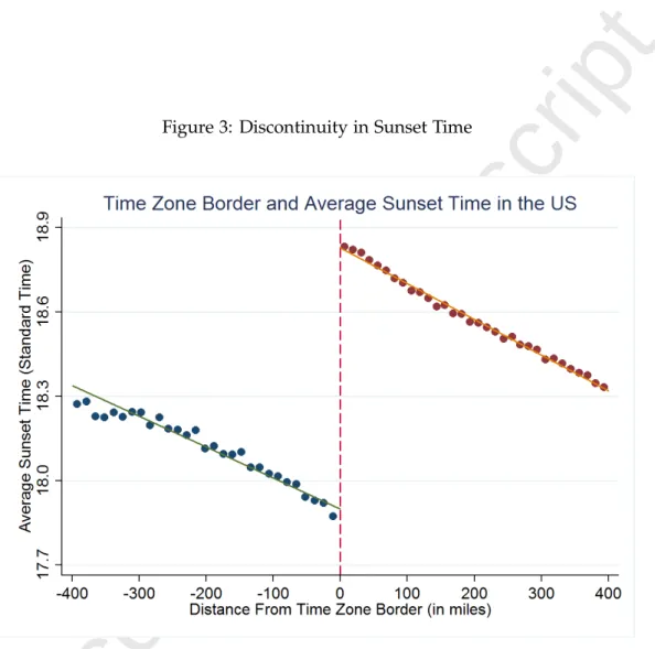
To analyze the effects of circadian rhythms disruptions on health and economic productivity, we exploit the sharp discontinuity in the relationship between sunlight and clock time at the time zone border. By construction, we observe a clear discontinuity in sunset time at the border (Figure 3), a discontinuity that is mirrored by the observed difference in average bedtime at the time zone border (Figure 4).13 This difference can be plausibly attributed to the delayed production of melatonin on the late sunset side of the border.
In Section4.1, we show that the difference in average bedtime generates significant differences
10More details on the methodology used by the CDC to compute prevalence estimates can be found here:
https://www.cdc.gov/diabetes/pdfs/data/calculating-methods-references-county-level-estimates-ranks.pdf
11The SEER*Stat statistical software provides an intuitive mechanism for the analysis of SEER and other
cancer-related databases. More information are provided here:https://seer.cancer.gov/seerstat
12Given the high number of missing values on acute myocardial infarction, coronary, angina disease and colorectal
cancer (jointly reduce the available counties by roughly 40%), we substituted missing observations using only the other four health variables (diabetes, obesity, breast and prostate cancer) to construct the index. However, if we use only the “balanced sample” (with all 8 health variables) or an index based only on the 4 variables always observed, point-estimates are very similar.
13We use data on the average bedtime of Jawbone’s sleep trackers users across US counties, publicly available on
the Jawbone website. Jawbone is one of the leading producers of wearable devices. The figure was downloaded from the Jawbone blog,https://jawbone.com/blog/circadian-rhythm/. We accessed the data on January 31, 2015
Accepted Manuscript
in sleeping behavior, as people on the late sunset side of a time zone boundary do not completely compensate for this difference by waking up later. This is especially true for workers who must cope with standard office hours and for people with children of school age.14Our identification strategy exploits this spatial discontinuity in sunset time and rests on the assumption that there are no discontinuities in observable and unobservable characteristics that may potentially confound the relationship of interest. Different from a standard regression dis-continuity design, we cannot simply compare all individuals living each side of a time zone border because this “unconditional approach” would compare individuals living at different lat-itudes (e.g., Tallahssee vs. Chicago, see Figure A.2) or around different time zone borders (e.g., Las Vegas vs. Atlanta). In order to exploit only variation across nearby counties, the main analy-sis controls for a set of geographic dummies that divide the United States in a grid of cells around US time zone boundaries and linearly control for latitude. In practice, we divide the US in 9 areas defined by the three time zones’ borders and three parallels (below the 34th parallel, between 34th and 40th parallel and above the 40th parallel). We also include controls for the annual average, the minimum and the maximum annual sunlight in a county (source: NOAA).
Ideally, one would compare only bordering counties on the two side of a time zone border. Since the ATUS data only include a limited number of counties (see Figures2and5), we cannot rely on such a comparison. However, in Section5, we show that our results are robust even if we only focus on the Central-Eastern border or if we further restrict the analysis to smaller quadrants across that time zone border, where most of the counties available in the ATUS are (i.e., Zone 1 and 2 in Figure 2). Moreover, when using county or zip code level data, we also run multiple linear, quadratic and cubic regressions focusing on counties within small latitude intervals and then average out the discontinuity effect along the border (see Section5.1 for further details).
The heterogeneity of our findings across socio-demographic and occupational characteris-tics, and the patterns of the outcomes analyzed support a causal interpretation of our findings. Consistent with our hypothesis that employed people, parents with children in school age, and individuals with early work schedules are more likely to be affected by circadian rhythms dis-ruptions because of their social schedules constraints (see Section 4.1). Moreover, the graphical analysis of the discontinuities in the outcomes studied closely mirrors the relationship between the timing of daylight and the distance from the time zone border.
3.3 Empirical Specification
More formally, we exploit the geographical variation in sunset time at the border, estimating the following equation:
yic=α0+α1LSc+α2f(Dc) +α3f(Dc) ∗LSc+Xic0 α4+C0cα5+Iic0α6+uic (1)
(2)
Accepted Manuscript
where yic is one of our outcomes of interest for the individual i in county c; LSc is an indicatorfor the county being on the late sunset side of a time zone boundary; Dc is the distance to the
time zone boundary, our “running variable” (or forcing variable), constructed using the county centroid as an individual’s location; the vector Xic contains standard socio-demographic
char-acteristics such as age, sex, race, education, marital status, nativity status, year of immigration, and number of children; and Cc are county characteristics, such as area fixed effects (the
geo-graphical cells described above), a linear control in latitude, control for the daily light exposure (yearly average, minimum and maximum) and an indicator for whether the respondent lives in a very large county.15 In our individual-level analysis using ATUS data we account for interview characteristics that might affect an individual’s sleeping behavior (Iic), such as interview month
and year, a dummy for whether the interview was conducted during DST, and two dummies that control for whether the interview was conducted during a public holiday or over the week-end. While our baseline geographical controls are crucial to ensure we compare nearby counties, the inclusion of socio-demographic characteristics and interview characteristics only serves the purpose of improving the precision of our estimates and to show that reassuringly our estimates are not sensitive to their inclusion. To this end, all tables show results with and without our covariates, while the graphical evidence of discontinuities in our main outcomes only conditions on a restricted set of baseline geographic controls.
Given the linear trend in the timing of sunset across the time zone boundary reported in Figure3, as baseline, we estimate a linear RD polynomial with a varied slope on either side of the cutoff. As robustness check, we also use (and compare) higher polynomial orders to control for the distance from the border (see Section5). Standard errors are robust and clustered according to the distance from each time zone border (10-mile groups).16 We also estimate this model using a local linear regression approach using both the standard and bias corrected inference procedure developed inCalonico et al.(2014) with kernel weights.
All estimates using the ATUS sample are weighted using the survey base weights which account for the differential probability of each household of being selected and for non-response. Bandwidth selection. We calculate the optimal bandwidth using the data-driven algorithm (MSE-Optimal bandwidth) proposed by Calonico et al., 2014. The optimal bandwidth varies depending on the outcome of interest (sleep, health index, etc.) and whether we include covariates. For instance for sleep duration, the optimal bandwidth ranges between 88 and 100 miles from the border. For this reason, in FiguresA.9 we show the robustness of our results to different bandwidth choices. Point estimates are relatively stable but standard errors increase as we get close to the border. In particular, when we restrict the bandwidth below 90 miles the number of observations declines very rapidly and, as a consequence, the estimated effects
15We control for the fact that in the case of very large counties, the distance based on the centroid might be a very
noisy approximation of the individual sunset time.
16We alternatively clustered standard errors at the county level. As we obtained smaller standard errors, we opted
Accepted Manuscript
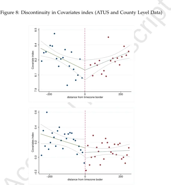
become no longer statistically significant at conventional levels. Note that, except for zip code level data, the bandwidth is calculated using the county centroid which is often several miles away from the time zone border, even when we restrict the analysis to counties bordering with a time zone boundary. In our baseline specification we use a bandwidth of 250 miles to ensure that areas on the late sunset /early sunset side of a time zone boundary do not overlap while maximizing our identification power. However, we also show that all our results are robust to the inclusion of state fixed effects and to the adoption of a smaller bandwidth (100 miles).Continuity in baseline covariates. To test the continuity assumption behind our RDD, we explore and test the continuity of many observed covariates at individual (FigureA.4) and aggregate level (FigureA.6) and in two pre-determined characteristics that should have not been affected by the treatment—namely respondents’ height and literacy rates in 1900 (before the official introduction of the time zones in 1918). We also find no evidence of discontinuities in employment status. It is however worth noting that employment and education may be potentially endogenous to health and sleep (Heissel and Norris,2017) and we cannot discard that with a larger sample and more precise measures of educational attainment, significant differences may arise. Despite the graphical inspection of discontinuity in covariates is useful and does not show any evidence of violation of the continuity assumption17, recent literature suggests that testing several individual hypothesis might lead to spurious rejections (Canay et al., 2017). For this reason, we increase the power of the analysis by testing the continuity of a “covariate index” (as inCard et al.,2012
and Kumar, 2018), which is constructed as the predicted outcome (sleep hours or the health
index) from a linear regression of the outcome variable on our large set of covariates (Figure8). Reassuringly we find no evidence of significant discontinuities in county level diseases (Figure
A.5) that should not be affected by circadian rhythms disruptions (e.g., HIV prevalence, brain cancer, cervical cancer, and any cancer among under 20). In addition, there is no evidence of discontinuities in birth outcomes, proxies for the quality of the health care supply and political orientation as measured by presidential votes (see the Appendix).
Manipulation of the running variable. The density of our running variable (distance from the time zone border) both in the ATUS and at county level does not show any sign of manipulation (Figure A.7). More formally, a density continuity test using the McCrary (2008) procedure was conducted and did not detect a discontinuity in the support of the running variable.18 However,
when analyzing county level data, which also include less populated counties, inference is more problematic. While there is no evidence of manipulation at the border, population density shrinks significantly on both sides, in close proximity to the border. Furthermore, counties in close proximity to the border are more likely to be rural and to have an older population (Figure
17Age is the only covariate for which the linear fit predicts a discontinuity at the time zone border. However, the
visual inspection of the data suggests that the discontinuity arises only as a consequence of the separated fit on the two sides of the cut-off. Furthermore, this is not a concern since in most specifications discussed later in the text we control non-linearly for age.
18The point estimate on a discontinuity in the distribution of the population is: -.032 (1.55) for county-level data;
Accepted Manuscript
A.8). Inference is further complicated by the fact that some labor markets span across the time zone border. In particular, there are a few commuting zones spanning across the Central and Eastern time zone border. For all these reasons, we show the sensitivity of our results to the exclusion of cross-bordering commuting zones and to the adoption of a “donut RD” (Barreca
et al.,2011) excluding counties with a centroid within 20 miles from the time zone border. It is
worth noting that when excluding counties within 20 miles from the border, the discontinuity in the treatment is substantially unchanged. The difference in sunset time within 20 miles is minimal, but by excluding these counties, we substantially reduce the measurement error due to spillovers within local labor markets/commuting zones.
4
Results
4.1 Sleep
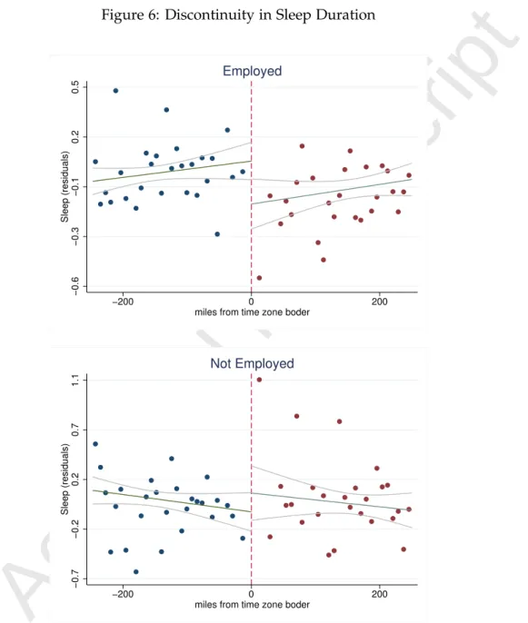
We first focus on the effects of the sharp discontinuity in the timing of sunlight at a time zone border on sleep duration (Figure 6). To compare only counties that are geographically close, we first regress sleep duration on our baseline geographical controls and then plot the residuals. Each point represents the mean residuals of sleep duration for a group of counties aggregated ac-cording to the distance from the border. We exclude Arizona and Indiana that did not adopt DST throughout the entire period under study (see Section 1.2).19 Purely for descriptive purposes, the
fitted lines are based on a linear fit on the two side of the discontinuity. As expected, we find ev-idence of a large discontinuity only for employed respondents. For this group, the discontinuity in sleep duration is of approximately 20 minutes. Interestingly, the linear trends on both sides of the border mirror the relationship between the timing of sunlight and the distance from the time zone border illustrated in Figure3. Tables1and2analyze the effects of the discontinuity in the timing of sunlight on sleep duration as described in equation (1). Our baseline estimate (column 1, Table1) coincides with the unconditional evidence reported in Figure6. After controlling for a set of socio-demographic, geographical and interview characteristics, the estimated effect of being on the late sunset side of the boundary (“late sunset border”) is approximately 19 minutes (column 2), reducing sleep duration by 0.2 standard deviations (see Table A.3). As some of the continental US states span multiple time zones (see FigureA.2), we re-estimate the model while including a full set of state fixed effects (column 3). Notably, the point estimates remain substan-tially unchanged. The coefficient is slightly higher when restricting the bandwidth to 100 miles (columns 4 and 5). There is also a large effect on the probability of sleeping less than 8 hours (column 6). Being on the late sunset side of the boundary decreases the likelihood of sleeping at least 8 hours by 7.8 percentage points, which is equivalent to approximately 15% of the mean of the dependent variable in the sample.20 The robustness of our estimates is also confirmed by
19When including these states, the figure is substantially unchanged, but the confidence intervals become wider.
However, we include Arizona and Indiana in the main analysis where we control for interview characteristics.
20As mentioned above, most respondents are interviewed over the weekend, and people tend to sleep longer over
Accepted Manuscript
the evidence reported in Table3(column 1–3) where we use the standard and the bias-corrected local-linear regression approach with kernel weights.The heterogeneity by employment status (see Figure6) arises because of differences in wak-ing time between employed and unemployed respondents (see Table 2). Regardless of their employment status, individuals on the late sunset side of the time zone border are always more likely to go to bed later (columns 3 and 4). The estimates show that being on the late sunset side of the boundary significantly increases the likelihood of being awake at midnight for both the employed (+41%) and the non-employed (+34%). However, employed respondents are less likely to adjust their waking time accordingly. There is no significant difference across the border in the likelihood of being awake at 7:30am for employed people (column 5). Conversely, non-employed people on the late sunset side of the time zone border adjust their waking-up time in the morning. Non-employed people on the late sunset side are 13 percentage points less likely to be awake at 7:30am, a 32% effect with respect to the mean of the dependent variable (column 6). These results are not sensitive to the choice of threshold or to the use of a continuous metric for bedtime and wake-up time (see TableA.5).
Consistent with the hypothesis that the results are in large part driven by working sched-ules’ constraints on sleep duration, we find that earlier working schedules corresponds to larger discontinuities at the time zone borders (Table A.4).21 More specifically, we find that among in-dividuals starting work before 7 am a one-hour increase in average sunset time decreases sleep duration by 36 minutes (column 1), while the effect for individuals starting work between 7 and 8:30 am is approximately 18 minutes (column 2). By contrast, we find that there is small or no effect on individuals starting work between 8:30 am and noon (column 3).22 However,
even among those starting work after 8:30 am, individuals who left children at school before 8 am sleep substantially less and there is a large and significant effect of sunset time (column 4). Specifically, among those entering work later in the morning, a one-hour increase in average sun-set time decreases sleep duration by 27 minutes for those who brought children to school before 8 am. Consistent with these findings, we find larger effects for people with children younger than 13 even when including the non-employed (TableA.6). We also find evidence of significant heterogeneity across sectors, with large effects for people working in public offices and in the financial sectors and close to zero for those working in the retail and wholesale sector (see Table
A.7). This is consistent with the fact that many shops and stores in the US open relatively late in the morning. Shopping malls open no earlier than 9am, and often around 10am.23 Reassuringly, we do not find discontinuities in the distribution of employment across sectors (TableA.8).
These findings suggest that delaying work and school start times may have important effects 8 hours and less than 6-hours.
21Note that to conduct this analysis, we restricted the sample to individuals who reported to work on the day of
the interview. As 50% of the ATUS sample is interviewed over the weekend and only 23% of the employed sample reported having worked over the weekend, the sample is substantially restricted.
22We classify individuals in these 3 categories to compare groups of similar size and based on the distribution of
working schedules.
Accepted Manuscript
on average sleep duration. When we analyze the entire ATUS sample, without restricting the analysis to counties within 250 miles from the time zone boundaries, individuals with early working schedules and/or whose children have early school start times sleep significantly less than individuals who are less likely to be constrained by social schedules in the morning (see Table A.9). Furthermore, the fact that the heterogeneity of the results presented in this section confirms our main hypotheses is reassuring and suggests that we are not confounding the effect of late sunset with that of other factors.As shown in Figure 2, using ATUS data we can only exploit a limited set of counties that lie mainly on the Northern and Central part of the border between the Eastern and Central time zones (Zone 1 and 2). As a robustness check, TableA.10 documents that the discontinuity in sleep duration is still precisely estimated when we focus our analysis only on the border between the Eastern and Central time zone or using only the northern part of this border (the region comprised between the 38th and the 45th parallel, Zone 1 of Figure2).
To assess the external validity of the results obtained using ATUS data we use county-level data drawn from the BRFSS survey on number of days without enough sleep in the month preceding the survey (see TableA.11). This analysis confirms the discontinuity in sleep duration across the time zone borders. The share of individuals reporting insufficient sleep —defined as reporting more than 14 days without enough sleep– is significantly higher in counties lying on the late sunset side of the time zone border. Furthermore, there is no-significant discontinuity in the share of individuals reporting insufficient sleep when focusing on the non-employed population.
Sleep Quality
Circadian rhythms disruptions may not only affect sleep duration, but also importantly affect sleep quality. While we do not have good measures of sleep quality, we used ATUS data to compute the number of times subjects woke up during night (number of sleep episodes) and the times subject reported to be in bed but sleeplessness. Conditional on overall sleep duration, indi-viduals on the late sunset side of the border tend to be more restless and to wake up more times at night (see TableA.12). However, the effects appear relatively small in magnitude. Individuals living in late sunset counties wake up 1% more times and tend to be restless 90 seconds more than their counterparts on the opposite side of the time zone boundary.
4.2 Health Outcomes
ATUS Data
As mentioned above, ATUS data contain limited information on body weight and self-reported health. Information on health status and body mass index is not available in all ATUS survey waves; thus, we have limited identification power. Nevertheless, we find evidence of sig-nificant discontinuities in the likelihood of reporting excessive weight (Table 4). There is also
Accepted Manuscript
evidence that individuals on the late sunset side of the time zone border are more likely to report poor health status, yet effects on poor health status are less precisely estimated.Employed individuals living on the late sunset side of a time zone border are 11% more likely be overweight with respect to the mean (column 1). They are also 5.6 percentage points more likely to be obese, approximately a 21% increase with respect to the mean of the dependent variable in the sample under analysis (column 2). Regarding self-reported health status (column 3), the effect is equal to nearly 2 percentage points but not statistically significant.24 Consistent with the effects on sleep, we find that the effect on weight are concentrated among those with early work schedules (see TableA.13). Figure A.9illustrates the sensitivity of our results to the bandwidth choice.
These estimates must be interpreted with caution. First, because of the ATUS sample re-strictions, these results are only representative of heavily populated counties where the work schedules constraints are likely to be more binding and sleep (and health) effects of social jetlag larger. In the Appendix, we show that the discontinuity in obesity is significantly smaller when considering aggregate data for all US counties because of the sample selection discussed in Sec-tion3. Second, these effects are likely to be the result of long-term exposure to sleep differences (caused by the different sunset time) on the two sides of a time zone border. In other words, what we measure is the average effect of a long-term exposure to differences in the timing of sunlight. These findings are consistent with the growing evidence that circadian misalignment and sleep debt are associated with metabolic and endocrine alterations that have long-term physiopatho-logical consequences (Spiegel et al., 1999). Moreover, the magnitude of the effects presented in Table4is comparable with the associations found in epidemiological studies. In particular,
Roen-neberg et al. (2012) find that an hour of social jet lag is associated with a 30% higher likelihood
of reporting overweight or obese status.25 Actually, our estimates are lower than what implied by these studies.
County Level Data
Given the limitations of the ATUS data, we explore alternative data sources using county level data drawn from the CDC. We restrict our attention to outcomes that previous research associ-ated with circadian rhythms disruptions and sleep deprivation: obesity, diabetes, cardiovascular diseases, and certain types of cancer (breast, colorectal, and prostate).26 In the main text, for space considerations, we report the effects on a composite index of health which we built stan-dardizing and summing the values of our health outcomes of interest. However, in the Appendix we report separate results for each health outcome (FiguresA.10-A.11and TablesA.14-A.17).
24Given the binary nature of our outcome variables, we also replicate our analysis using the probit model. The
marginal effects are identical up to the fourth decimal place.
25Similarly,Moreno et al.(2006) find that among Brazilian truck drivers sleep duration<8 h per day was associated
with a 24% greater odds of obesity, whileHasler et al.(2004) find that every extra hour increase of sleep duration was associated with a 50% reduction in risk of obesity. Evidence from animal studies also finds large effects of partial sleep deprivation on weight (Knutson et al.,2007).
Accepted Manuscript
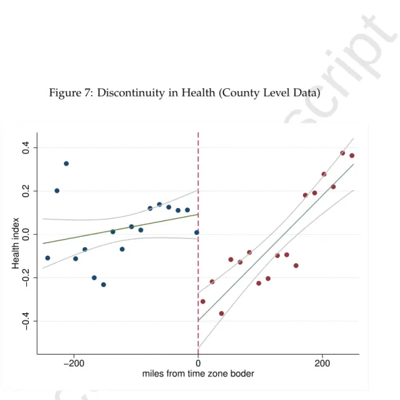
In the graphical analysis (Figure7), we only control for our baseline geographic controls and exclude the commuting zones spanning across time-zones. The discontinuity at the border is remarkably evident. If we exclude the two data points over 200 miles away from the timezone on the east side, health trends would exhibit a parallel pattern on both sides of the border, mirroring again the relationship between the timing of sunlight and the distance from the time zone we have shown before (Figure3). This is more clear when restricting the analysis to the more densely populated Eastern-Central time zone border (Figure A.3). Furthermore, it is reassuring the we do not observe similar trends for our covariates index (bottom part of Figure8).The estimated unconditional discontinuity at the time zone border in the health index is al-most .5 standard deviation (Table5, column 1). The coefficient becomes smaller when including sociodemographic controls and when restricting the bandwidth to 100 miles. However, the point estimate remains economically important and statistically significant pointing at a .3 standard deviation difference in health across the time zone border. The result is also robust to the inclu-sion of state fixed effects. As for sleep, we show the robustness of our result to non-parametric methods (column 4–6) of Table3.
4.3 Economic Effects
Economic costs: a Back of the Envelope Calculation
Based on existing estimates of the health care costs of obesity, diabetes, acute myocardial infarctions, strokes and breast cancer, we estimated an average annual cost by at least 2.35 billion dollars (approximately $82 per capita, in 2017 $) per year (see Table A.18). We obtained these estimates by multiplying the per capita costs of these diseases by the effects of social jetlag shown in TableA.14and the population living in areas on the late sunset side of the time zone border.27 This is only a coarse attempt to quantify the health care costs associated to the circadian rhythms’ disruptions induced by the time zone border. It is also a lower bound estimate as we limit the analysis to the set of outcomes studied in this paper and because we calculated the costs only for the 18-65 working population.
To gauge an idea about the potential effects on productivity that may be related with absen-teeism and presenabsen-teeism induced by the circadian misalignment, we use the estimates ofHafner
et al.(2016). Based on a UK Britain’s Healthiest Workplace survey, they find that a worker
sleep-ing less than six hours loses approximately six worksleep-ing days due to absenteeism or presenteeism per year and a worker sleeping six to seven hours loses on average 3.7 working days more per year. We find that workers living on the late sunset side of the border are 4.5% more likely to sleep less than 6 hours and 2.7% more likely to sleep between 6 and 7 hours (TableA.1). Using these results and weighting them by the working population living on the late sunset side of the border, we estimate a loss of approximately 4.40 million days of work (1.3 hours per capita) per
27Note that the estimates shown in Table A.15 measure the effect at the border. For the back of the envelope
calculation we assumed that the effects linearly decline with distance. We weighted the effects considering intervals of 50 miles (0-50,50-100, 100-150, 150-200 and 200-250) and weighting by the population living in each of these intervals.
Accepted Manuscript
year. Based on median hourly wage in 2015 of $17.40 that is equivalent to 612.9 million dollars ($23 per capita loss per year).Income per Capita
Individual health is a major factor of economic performance and productivity (Grossman,
1972;Mitchell and Bates,2011). Sleep-deprivation has been associated with worsened cognitive
performance (Van Dongen et al.,2003). Furthermore, the negative health effects illustrated in the previous section may substantially affect individual productivity (see for instanceCawley et al.,
2007). Recently, the potential beneficial effects of sleep on productivity have led some companies to introduce incentive schemes aimed at promoting employees’ sleep and sleep is now one of the three pillars of U.S. Army Performance Triad.28
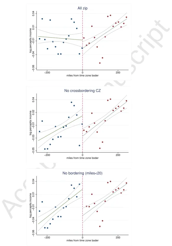
Using zip code level data drawn from the American Community Survey (ACS) 2010–2014, we tested for the presence of discontinuities in income per capita. As mentioned above, zip codes that are very close to the border may be in the same commuting zone or same labor market of their bordering zip codes on the opposite side of the border biasing our results. Furthermore, time zone borders were often drawn in rural areas characterized by a lower population density and a different demographic composition of the population (see FigureA.7andA.8). The differ-ent characteristics of areas at the border may increase noise and attenuation bias when we use aggregate-level data. In addition, within commuting zones spanning across a time-zone bound-ary mobility costs are likely to be low and arbitrage should eliminate any wage differential. Indeed, we find no significant differences in income across the time zone border, when including commuting zones spanning over multiple time zones. However consistent with our hypothesis, in Figure 9 we show that the evidence of a discontinuity in income per capita becomes more clear as we exclude from the figure zip codes belonging to commuting areas spanning across the time zone border or alternatively exclude zip code with a centroid within 20 miles from the time zone border. Table 6presents the results of the regression discontinuity estimates. In these esti-mates, we also include controls for standard demographic characteristics (shares by age group, race, sex, education, population size, and rural status) and an indicator for commuting zones spanning across the time zone border, significantly increasing precision. The estimated effect at the border implies a 3 percentage points decrease in per capita income. This result is robust to the choice of bandwidth (250 vs. 100 miles), to the inclusion of state fixed effects (columns 2 and 4) and to the exclusion of zip codes within 20 miles from the border (column 5).
The magnitude of our result is comparable to what found by (Gibson and Shrader,2018) who estimate that a one-hour increase in location-average weekly sleep increases earnings by 4.5% in the long run. However, our analysis suggests that these significant differences in income emerge only when comparing counties belonging to different commuting zones. It is however worth noting that our results are not directly comparable given the different identification strategies
28http://www.huffingtonpost.com/entry/aetna-pays-employees-to-sleep-more_us_
Accepted Manuscript
adopted. We identify a local average treatment effect at the border. Furthermore, the difference in the results may also be explained by the different data used for this analysis, as (Gibson andShrader,2018) use ATUS data.
5
Robustness Checks
In this section, we present additional tests to support the validity of our identification strategy and to verify the robustness of our results.
First, we report the results of conventional and biased corrected local linear regression-discontinuity estimates on triangular kernel for our main outcomes of interest (Table 3). To conduct this analysis, we follow the procedure implemented by Calonico et al. (2014). The re-sults are overall in line with our baseline estimates.
Second, we re-estimate the models discussed in Table 1 using alternative metrics for sleep duration (TableA.1). Column 1 replicates the results presented in column 1 of Table1. We show that the coefficient is substantially unchanged if we include afternoon naps (column 2). We then focus on non-linear metrics of sleep duration typically used in medical studies (Ohayon et al.,
2013; Markwald et al., 2013). Individuals on the late sunset side of the time zone border are 4
percentage points more likely to report less than 6 hours sleep (column 3), 8 percentage points less likely to report at least 8 hours’ sleep (column 4), and 3 percentage points less likely to report sufficient but not excessive sleep (column 5). We find no differences in naps measured as the total amount of time slept between 11am and 8pm (see column 6). However, when restricting to weekends there is some evidence of compensatory behavior (about 7 minutes additional napping) for people leaving on the late sunset time (TableA.2). Although this effect is relatively small in magnitude, the result is consistent with the hypothesis that work schedules may inhibit any adaptive behavior.
We also investigate the presence of seasonality in the discontinuity at the time zone borders. We find no evidence of significant differences in the discontinuity in sleep duration in summer and winter time (during daylight saving time and standard time). As expected, individuals tend to go to bed later in the summer. However, there is no systematic difference across the border and if anything, the difference in sleep duration between individuals living in early and late sunset counties is smaller during summer time (see TableA.19). Similarly, we find no significant differences between northern and southern regions. This result is consistent with the fact that the process of melatonin secretion is affected by the duration of sunlight throughout the day, with a phase-delay in melatonin secretion when the days are shorter (Luboshitzky et al., 1998). The change in melatonin secretion across seasons or latitudes can explain the lack of seasonal or geographical heterogeneity in the effect of interest.
Using ATUS data we cannot identify counties or metropolitan areas with fewer than 100,000 residents. However, we examine the heterogeneity of our effects on sleep by the size of the metropolitan area of residence (TableA.20). The effect is larger in more populated metropolitan
Accepted Manuscript
areas, likely reflecting differences in the occupational and demographic characteristics of indi-viduals living in smaller cities but also the longer commuting that many people may face in the morning in large metropolitan areas. To ensure that the results are not driven by one particular state (metropolitan area), we tested and confirmed the robustness of our main results to the ex-clusion of one state (metropolitan area) at a time from our estimates (results are available upon request).Measurement error in the weight and height variables is a natural concern. Since height and weight are self-reported in the ATUS, and previous studies documented systematic reporting error in such self-reports, as a robustness check we adjusted body mass for measurement error following Courtemanche et al. (2015). Specifically, we used the National Health and Nutrition Examination Surveys (NHANES) as validation sample and relatively weak assumptions about the relationship between measured and reported values in the primary and validation datasets. As expected, the point estimates using the corrected BMI are very similar to those reported in the main text (coef., 0.062, std.err., 0.032 for overweight status; and coef., 0.063, std.err., 0.030 for obesity status).
Using the ATUS data we analyzed the heterogeneity of the results on weight and health status by work start times (TableA.13). Point estimates for overweight and obesity are proportional to the results obtained on sleep (Table A.4). Point estimates are approximately twice the average effect for early work schedule workers (5-7 am). Unfortunately, standard errors are very large as the sample size available for this analysis is very small. Despite this, the point estimates for early schedule workers are still statistically different from zero. These results could also be explained by the presence of non-linearity as those with very early schedule sleep much less on average. Unfortunately, given the limitation of our data, we cannot disentangle the presence of non-linearity from a “compliance” explanation—where the estimated effect is driven by those that are constrained and then more likely to be exposed to the negative effects of a late sunset.
We tested for the optimal polynomial order by comparing our local linear regression approach with higher polynomial orders, up to the fourth, on the full (feasible) bandwidth (280 miles). Table A.21shows that the point estimates are relatively stable up to the third order polynomial (around 0.3 of an hour, namely 18 minutes), while they become unreasonably large using the forth order polynomial (50 minutes). As shown in Figures3and6 the linear approximation for the distance from the time zone seems to fit the data very well. Moreover, Figure6does not show evidence of a discontinuity of more than 20 minutes. This suggests an overfitting problem when using higher order polynomial. The Bayesian information criterion (BIC) is minimized using the forth order polynomial but the local linear regression is clearly preferred over the quadratic and the cubic polynomials.
A natural concern is that residential sorting across the time zone border will create correlation between unobservable individual characteristics and individual residence. As largely discussed in Section 3.2, the presence of commuting zones spanning across a time zone border and the westward movement of time zone border complicates the analysis in the close proximity to the