HAL Id: hal-02429520
https://hal.archives-ouvertes.fr/hal-02429520
Submitted on 18 Mar 2020
HAL is a multi-disciplinary open access
archive for the deposit and dissemination of
sci-entific research documents, whether they are
pub-lished or not. The documents may come from
teaching and research institutions in France or
abroad, or from public or private research centers.
L’archive ouverte pluridisciplinaire HAL, est
destinée au dépôt et à la diffusion de documents
scientifiques de niveau recherche, publiés ou non,
émanant des établissements d’enseignement et de
recherche français ou étrangers, des laboratoires
publics ou privés.
CABRI Power Transients Analysis
Olivier Clamens, Patrick Blaise, Jean-Pascal Hudelot, Johann Lecerf,
Bertrand Duc, Laurent Pantera, Bruno Biard
To cite this version:
Olivier Clamens, Patrick Blaise, Jean-Pascal Hudelot, Johann Lecerf, Bertrand Duc, et al.. Coupled
Experimental and Computational Approach for CABRI Power Transients Analysis. IEEE
Transac-tions on Nuclear Science, Institute of Electrical and Electronics Engineers, 2018, 65 (9), pp.2434-2442.
�10.1109/tns.2018.2847331�. �hal-02429520�
Coupled experimental and computational approach
for CABRI power transients analysis
Olivier Clamens, Patrick Blaise, Jean-Pascal Hudelot, Johann Lecerf, Bertrand Duc, Laurent Pantera,
and Bruno Biard
Abstract—CABRI is an experimental pulse reactor, funded by the French Nuclear Safety and Radioprotection Institute (IRSN) and operated by CEA at the Cadarache research center. It is designed to study fuel behavior under RIA (Reactivity Initiated Accident) conditions. In order to produce the power transients, reactivity is injected by depressurization of a neutron
absorber (3He) situated in the so-called “transient rods” inside
the reactor core. The CABRI reactivity injection system allows us to generate structured transients based on specific sequences of depressurization. For such transients, the time difference between the openings of two valves of the reactivity injection system has an important impact on the power pulse shape. A kinetic point code, SPARTE, was developed in order to replace the older DULCINEE code dedicated to the modeling and prediction of CABRI power transients. The SPARTE code includes new
models of 3He depressurization based on CFD calculations,
variable Doppler coefficient based on Monte Carlo calculations and variable axial neutron flux profile. The density and Doppler models have a large impact on power transient prediction. For low initial pressure transients, the major uncertainty comes from
the reactivity injected by the 3He depressurization. For high
initial pressure transients, the 3He heating during the power
pulse (“TOP effect”) is responsible of an additional injection of reactivity that needs to be modeled precisely.
Index Terms—CABRI, Power transients, SPARTE, multi-physics
I. INTRODUCTION
C
ABRI is an experimental pulse reactor funded by the French Nuclear Safety and Radioprotection Institute (IRSN) and operated by CEA (Commissariat `a l’ ´Energie Atomique et aux ´Energies Alternatives) at the Cadarache research center. Since 1978, the experimental programs have been aiming at studying the fuel behavior under Reactivity Initiated Accident (RIA) conditions. In order to study PWR high burn up fuel behavior under such transients, the facility was modified to accept a pressurized water loop in its central part, able to reproduce thermal-hydraulics characteristics rep-resentative of PWR nominal operating conditions (155 bar, 300◦C). This project, which began in 2003 and supported first commissioning tests from October 2015 to March 2017, was driven within a broader scope including both an overall facility refurbishment and a complete safety review. The global modifications have been conducted by the CEA project team and funded by IRSN, which is operating and managing the O. Clamens, J. Lecerf, J-P. Hudelot, B. Duc, L. Pantera DEN CAD/DER/SRES CEA Cadarache, Bt 721. 13108 St Paul Lez Durance, France e-mail: [email protected].P. Blaise, DEN CAD/DER/SPEX CEA Cadarache, Bt 238. 13108 St Paul Lez Durance, France.
B. Biard, IRSN/PSN-RES/SEREX Cadarache, BP3 13115 Saint-Paul-Lez-Durance Cedex, France.
CIP experimental program (CABRI International Program), in the framework of an OECD/NEA agreement. The CIP program will investigate several UOx and MOX LWR spent fuel samples under RIA conditions, with a foreseen completion by the end of 2023. Power transients are generated by a dedicated so-called transient rods system [1] allowing the very fast depressurization of 3He tubes positioned inside the
CABRI core.
The first part of this paper is dedicated to the description of the CABRI power transients. In a second part, we will address the prediction of those transients and speak about the models that were added to the newly developed SPARTE code in order to improve the prediction precision. This paper also focuses on experimental and calculation uncertainties and their impact on the CABRI power transients.
II. CABRIPOWER TRANSIENTS A. Transients measurement
Two types of transients are needed for the CIP program. First ones are natural transients described in the following paragraph. Second ones are structured transients described in the next paragraph.
Specific boron-lined ionization chambers are used for mea-suring high power levels during steady states or during power transients [2]. In the case of power transients, several boron ionization chambers, located at increasing distances from the core (see Fig. 1), are used to cover the whole power range (i.e. from 100 kW to ∼ 20 GW). More details can be found in references [3]–[5].
B. Natural transients
Natural transients consist of single pulses with a FWHM (Full Width at Half Maximum) of approximately 10 ms. They are made by single opening of the high flow rate channel (VABT01, see Fig. 2).
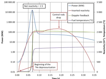
One example of natural transient is reproduced on Fig. 3. The reactivity injected by 3He depressurization causes a
power increase. The energy deposited in the fuel leads to a temperature increase. When the injected reactivity is bal-anced by Doppler and other reactivity feedbacks, the power decreases until a new equilibrium is reached. The reaction is then completely stopped by dropping the control rods. The parameters of the experiment are the control valve aperture (VABT03), the initial 3He pressure, the rod drop instant, the initial stabilized power and the initial system temperature. The transient shape is mostly depending on the valve aperture and the initial pressure. The energy deposited in the core during
Fig. 1. Experimental boron ionization chambers near CABRI core
Discharge reservoir (~1000 l) Control valve VABT04 Fast opening valve VABT02
Sensor for pressure measurement 4 Transient rods Control valve VABT03 Fast opening valve VABT01 Collector
Fig. 2. Main components of the CABRI transient rods
the power transient is also controlled by the rod drop instant. The initial temperature is really important, in order to know the exact3He quantity in transient rods.
C. Structured transient
In order to be representative of other RIA conditions of NPPs (Nuclear Power Plants), it is necessary to be able to increase the FWHM of the transient. This can be done by opening successively the fast opening valves of the low and then of the high flow rate channels. When the net reactivity is close to 1 $, the high flow rate channel is opened to compensate during a short instant the reactivity feedbacks by a
0 500 1 000 1 500 2 000 2 500 3 000 3 500 0.01 0.10 1.00 10.00 100.00 1 000.00 10 000.00 100 000.00 0.00 0.05 0.10 0.15 0.20 0.25 0.30 0.35 R ea ctivi ty (10 -5), Temp er atu re ( °C) P o w er ( MW ) Time (s) Power (MW) Inserted reactivity Doppler feedback Fuel temperature (°C) Beginning of the 3He depressurization Net reactivity ≈ 1 $ Control rods drop
Fig. 3. Natural power transient and reactivity analysis
fast reactivity insertion. It allows thus a more important energy deposit during the pulse. The adjustment of the time difference between the openings of the fast opening valves allows us to generate so called “structured transients” characterized by FWHM varying from 20 to 80 ms.
III. IMPACT OF TIMING FOR STRUCTURED TRANSIENTS The experimentalists issue is to generate, with the CABRI core, the ideal power transient for the experimental purposes. One goal of the reactor commissioning tests performed in the first 2017 quarter was to generate power transients with a FWHM of 30 ms with a sufficient energy deposit. This can be achieved with structured transients as described in the last paragraph. In order to reach experimental goals, the transient parameters have to be precisely mastered. Considering an initial power of 100 kW, the different parameters are:
• The apertures of the two control valves (VABT03 and VABT04),
• The 3He initial pressure,
• The opening time of the two fast opening valves
(VABT01 and VABT02).
A. The timing issue
The uncertainties on pressure and apertures are really small. However, an uncertainty exists on the time needed for the fast valves to open. A standard deviation of approximately 2 ms was observed on the opening time of VABT01. A major improvement was carried out during the CABRI renovation in order to reduce and master the uncertainty linked to the VABT02 opening. In the past, the second valve opening signal was triggered when pressure reached 90 % of its initial value. The limitation of this method is that at the beginning of the depressurization, many oscillations are recorded. Those variations are linked to the different 3He flows coming from different locations of the circuit. Those variations are repro-ducible from a depressurization to another and can also be observed in detailed CFD calculations. Few milliseconds of uncertainty were then added to the standard deviation observed
3.5 3.7 3.9 4.1 4.3 4.5 4.7 4.9 5.1 5.3 5.5 0.365 0.366 0.367 0.368 0.369 0.37 0.371 Pr essu re (b ar) Time (s) 3He depressurization 1 3He depressurization 2 ∆𝑡=0.9 𝑚𝑠±0.25 𝑚𝑠
Fig. 4. Difference between 2 VABT01 opening times on 2 commissioning tests in the same conditions
for VABT01. The opening command of the second valve is now given by the specific control device when pressure reaches 75 % of its initial value. In that zone, no variations are observed, only 0.25 ms of uncertainty can be added due to the acquisition rate. On Fig. 4, we can observe the time gap between the 2 openings of the high flow rate channels on two “structured” transients that have the same parameters. This gap is under 1 ms, but still has a real impact on the transient shape.
B. The impact on power transients
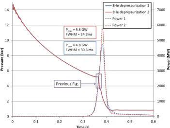
The difference between the 2 power transients is depicted on Fig. 5. The two peaks climax at the same moment. However, the maximum powers (1 GW gap) and FWHM (6 ms gap) are different. When the opening time comes faster, the power is going higher and the transient is a little thinner. Nevertheless, the energy deposited in the core is very close in the 2 cases. Before every irradiated fuel test, a campaign of approximately 10 transients without test rod in the central cell is performed. It results an uncertainty of approximately 5 ms on the FWHM for transients of 30 ms FWHM.
IV. SPARTE,A POINT KINETICS CODE DESIGNED FOR CABRI
In order to analyze and to predict the CABRI power transients, a calculational approach is necessary. Currently, kinetics aspect is calculated by the DULCINEE [6] code and thermal-mechanics safety calculation are done by the SCANAIR [7] code. A new code is being developed in order to improve the prediction capacity as for kinetics aspects. The goal of this code is to improve the prediction of the CABRI power transients in terms of reached maximal power, FWHM, energy deposited and timing of the peaks.
SPARTE is a new code adapted to CABRI transients. It is based on the DULCINEE point kinetics code. Surrogate mod-els and modifications of the datasets have been added in order to be more representative of the physical conditions. Surrogate
0 1000 2000 3000 4000 5000 6000 7000 0 2 4 6 8 10 12 14 0 0.1 0.2 0.3 0.4 0.5 0.6 P o w er ( MW ) Pr essu re (b ar) Time (s) 3He depressurization 1 3He depressurization 2 Power 1 Power 2 Pmax = 4.8 GW FWHM = 30.6 ms Pmax = 5.8 GW FWHM = 24.2ms Previous Fig.
Fig. 5. Comparison of the two power transients resulting from the 2 similar depressurizations
models are based on Best-Estimate calculations (CFD [8] and Monte-Carlo [9]) and built with Artificial Neuronal Networks with URANIE [10]. In this part, we will present the four main improvements and their impact on the transient prediction:
• Surrogate model of the 3He density in transient rods
during depressurization,
• Variability of the Doppler coefficient as a function of the transient of power conditions,
• Axial neutron flux profile depending on the control rods position,
• Variability of the prompt neutron life time during power transients.
In every part, improvements will be added one by one on an example of transient. This example is a “natural” transient based on a depressurization beginning at 7 bar of3He with a
full aperture of the high flow-rate channel.
A. Surrogate model of helium density
CFD calculations have been made in order to evaluate the Helium-3 density in the transient rods volume. A surrogate model estimating the3He density in the transient rods has thus
been developed and implemented [8]. The3He density in the
transient rods is more relevant than the3He pressure measured
by the sensors (see Fig. 2) to take into account the impact of the3He temperature in the reactivity injection calculation. This model replaces the old model based on analytical solution of the 3He depressurization (demonstration in [11]):
P (t) = P0( m(t) m0 )γ = P0[Bt + 1] −2γ γ−1 (1)
Fig. 6 represents the difference between the density evolu-tion and the pressure evoluevolu-tion. We can see that the pressure evolution is much faster than the density evolution. So, the reactivity injection calculated with the pressure curve is also much faster. That is why, the real power transient comes after the power transient calculated with the pressure model. The density model has a big effect on the transient shape and needs to be added to the code.
0 0.1 0.2 0.3 0.4 0.5 0.6 0.7 0.8 0.9 0 0.02 0.04 0.06 0.08 0.1 0.12 0.14 0 5000 10000 15000 20000 25000 Density (kg/m3) Power (MW) Time (s) Pressure model Density model Power measured Power| model Off Power| model On
Fig. 6. Effect of density model on the power transient calculation
B. Variability of the Doppler coefficient
Neutronics calculations of the CABRI core using the French stochastic TRIPOLI4 [9] code show that the Doppler coef-ficient is varying with CABRI power transients conditions. The Doppler coefficient varies with fuel temperature and core poisoning due to Helium-3 and to control rods. This can be explained by the hardness of neutron spectrum. The 3He
neutron absorption is very effective in thermal condition. The more3He pressure in the transient rods important is, the harder the neutron spectrum is. The hardness of the neutron spectrum is also increasing with the elevation of the fuel temperature.
An Artificial Neuronal Network was created using the results of TRIPOLI4 simulations of the CABRI core. The parameters of the surrogate model are:
• The elevation “z” of the control rods (Hafnium),
• The density “d” of3He is the transient rods,
• The Fuel temperature “T” (UO2)
700 simulations were completed based on Latin hypercube sampling. The resulting surrogate model computes the mul-tiplication factor depending on the different parameters. In SPARTE, the Doppler coefficient is on the integral form and is defined as follows:
ρD= AD∗ (
√
T −pT0) (2)
We can also write the Doppler reactivity depending on the multiplication factor k as follows:
ρD= ρ(T ) = ρ(z, d, T ) − ρ(z, d, T0) (3)
Where:
ρ =k − 1
k (4)
From (2),(3) and (4) we can deduce (5):
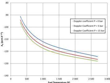
AD= k(z,d,T )−1 k(z,d,T ) − k(z,d,T0)−1 k(z,d,T0) √ T −√T0 (5) Fig. 7 shows the evolution of the Doppler coefficient with temperature at different 3He pressures in the transient rods, the control rod insertion being fixed. The Doppler coefficient increases in absolute value with fuel temperature and core
-140 -130 -120 -110 -100 -90 -80 0 500 1 000 1 500 2 000 2 500 3 000 AD ( pcm .K -1/ 2) Fuel Temperature (K)
Doppler coefficient P = 0 bar Doppler Coefficient P = 5 bar Doppler Coefficient P = 15 bar
Fig. 7. Variability of the integral Doppler coefficient in CABRI core depending on fuel temperature and3He density
0 200 400 600 800 1000 1200 1400 1600 1800 2000 0 0.02 0.04 0.06 0.08 0.1 0.12 0.14 0 2000 4000 6000 8000 10000 12000 14000 16000 18000 Doppler reactivity (pcm) Power (MW) Time (s) Doppler fb| Ad = cste Doppler fb| Ad = var Power measured Power| model Off Power| model On
Fig. 8. Effect of Doppler model on the power transient calculation
poison quantity. So, during a transient, the Doppler coefficient decreases because of the3He depressurization, and in the same
time increases because of the fuel temperature elevation. In the SPARTE code, the Doppler coefficient is then calculated as in (5), using the surrogate model of multiplication factor. The Doppler coefficient is calculated at each time step and for each fuel mesh.
On Fig. 8, is represented the influence of the Doppler coefficient model added to the SPARTE code. We can observe that the Doppler reactivity feedback is increasing higher with the model than for a constant value of the Doppler coefficient. It is due to an elevation of the absolute value of the coefficient with increasing temperature. The addition of the Doppler surrogate model in the simulation reduces the FWHM of the calculated power transients.
C. Axial neutron flux distribution
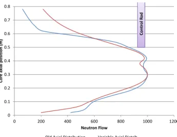
The axial neutron flux distribution is taken into account in the SPARTE code. It is used to calculate the energy deposition depending on the height of the fuel. It is also used to evaluate
0 0.1 0.2 0.3 0.4 0.5 0.6 0.7 0.8 0 200 400 600 800 1000 1200 Cor e a xial p os itio n (m) Neutron Flow
Old Axial Distribution Variable Axial Distrib
Con tr ol R od Con tr ol R od
Fig. 9. Calculated axial distribution compared to the old axial distribution
0 200 400 600 800 1000 1200 0 0.02 0.04 0.06 0.08 0.1 0.12 0.14 0 2000 4000 6000 8000 10000 12000 14000 16000 18000 Fuel temperature (C) Power (MW) Time (s)
Fuel T| model Off Fuel T| model On Power measured Power| model Off Power| model On
Fig. 10. Effect of axial distribution on the power transient calculation
the axial distribution of the reactivity feedbacks (Doppler, void, temperature) . The CABRI case is specific because of the reactivity injection system. The control rods insertion, constant before triggering the depressurization and during the resulting pulse, until a manual scram order is initiated, depends at the first order on the initial 3He density in the transient
rods. Its dependency on the core cooling water temperature is secondary. That is why, the axial profile needs to be calculated for every calculation. Before the recent TRIPOLI4 calculation, the axial power profile in DULCINEE was coming from calculations of the hot channel near the control rods. The axial power distribution was therefore so low on the top of the core in the old axial profile (see Fig. 9). In the SPARTE code, a surrogate model based on the TRIPOLI4 calculations was added to calculate the core averaged axial power profile depending on the control rods insertion.
We can see that in this case, the new axial distribution has a moderate influence on the power transient shape. The axial neutron flux distribution is flatter, so that the temperature is better distributed. The Doppler reactivity feedback is then a little higher. This reduces slightly the maximum power (see
2.47e-05 2.48e-05 2.49e-05 2.5e-05 2.51e-05 2.52e-05 2.53e-05 2.54e-05 2.55e-05 0 0.02 0.04 0.06 0.08 0.1 0.12 0.14 0 2000 4000 6000 8000 10000 12000 14000 16000 18000
Neutron life time (s)
Power (MW)
Time (s)
Neutron life time cste Neutron life time var Power measured Power| model Off Power| model On
Fig. 11. Effect of neutron lifetime variability on the power transient calculation
Fig. 10).
D. Variability of neutron lifetime
The CABRI transients are characterized by a rapid with-drawal of the3He neutron absorbers, uniform within the core volume. We can easily assume that this withdrawal is responsi-ble of an extension of the neutron life time. TRIPOLI4 is aresponsi-ble to calculate kinetics parameters (effective neutron generation time “Λef f” and effective delayed neutron fraction “βef f)
thanks to the Iterated Fission Probability method (IFP) [12]. The calculations demonstrate the variability of the neutron life time. The most influent parameter is the 3He density. The
second one is the control rods insertion.
The impact of the neutrons life time is presented on Fig. 11. We can observe that the neutrons lifetime is increasing with depressurization of the3He. The neutrons lifetime being lower than reference at the beginning of the transient, the power peak arises shortly before the previous calculation. However, the neutrons life time staying close to the reference, and the impact on the transient calculation is low.
E. TOP effect model based on experiments and CFD SPARTE’s last improvement consists in modeling the TOP effect. This effect is detailed in [8]. The TOP effect comes from3He heating during power transients. As power increases, the thermal neutron flux also increases. So, the neutron absorp-tion by 3He intensifies. This reaction produces two charged
particles : proton and tritium. One part of their energies is deposited in the 3He gas by ionization before reaching the
metallic wall of the transient rods. Denser is the gas, higher the probability of ionization is and more important the deposited energy is. The direct effect of this energy deposit is that the gas temperature increases. A temperature increase is equivalent to a pressure increase. The differential pressure between rods and flow channels implies a faster depressurization of helium from the transient rods. This finally implies a rise of the reactivity injection speed. A surrogate model computing a deviation of the depressurization rate during power increasing was added to the code.
0 0.1 0.2 0.3 0.4 0.5 0.6 0.7 0.8 0.9 0 0.02 0.04 0.06 0.08 0.1 0.12 0.14 0 2000 4000 6000 8000 10000 12000 14000 16000 18000 Density (kg/m3) Power (MW) Time (s)
3He density| TOP Off 3He Density| TOP On Power| measured Power| TOP Off Power| TOP On
Fig. 12. Effect of the TOP effect model on the power transient calculation
The impact of the TOP effect is presented on Fig. 12. As we can see, the TOP effect model brings a deviation to the density evolution curve during the transient. The supplemen-tary reactivity inserted through the TOP effect completes the prediction of the transient.
F. Comparative tables
In this paragraph, the successive elaborated models are tested on different power transients. Four criteria are compared to the experiment:
• The maximum power “Pmax” of the transient,
• The Full Width at Half Maximum “FWHM” of the pulse, • The energy “E” deposited in the core after 1.2 s, • The instant of the peak “tpeak”.
All the transients compared are performed by single opening of a channel. Four tables show the four chosen examples :
• A transient with low initial pressure (1.3 bar) and the maximum aperture of VABT03 (high flowrate channel) (Table I),
• A transient with a middle initial pressure (4 bar) and a low
aperture of VABT04 (low flowrate channel) (Table II),
• A transient with a relatively high initial pressure (7 bar)
and the maximum aperture of VABT03 (Table III),
• A transient with the maximal initial pressure (∼ 14.5 bar) and a low aperture of VABT04 (Table IV).
For the four cases, the same approach is used. First, the measurement is presented. Then, a calculation shows the result of SPARTE with the 4 models presented dis-activated. The different models previously presented are then added one by one to the calculation. The last line of each table corresponds to the calculated power transient with all models activated.
We can observe that in all cases, the density evolution model and the Doppler coefficient model are the most influent on transient calculations. The density model brings the calculated peak closer to the measured peak in the time. The Doppler coefficient is higher than the reference in cases of high power (Table III), the calculated power being then lower. In all cases the Doppler model has for effect to reduce the FWHM. It is due to the elevation of the fuel temperature during the power
TABLE I
LOW INITIAL PRESSURE(1.3BAR)TRANSIENT
Models Pmax(MW) FWHM (ms) E (MJ) tpeak(ms)
Measurement 127 89.9 16.9 201 Calc 0 469 48.2 35.2 141 + density 297 63.9 28.9 191 + Doppler 316 61.8 29.7 191 + Ax dist 304 61.8 28.7 191 + Λef f 302 62.3 28.6 191 + TOP 302 62.3 28.6 191 TABLE II
MIDDLE INITIAL PRESSURE(4BAR)TRANSIENT
Models Pmax(MW) FWHM (ms) E (MJ) tpeak(ms)
Measurement 546 48.4 56 436 Calc 0 743 44.8 99 366 + density 472 57.4 66 434 + Doppler 502 54.3 64 434 + Ax dist 489 54.4 63 434 + Λef f 486 54.3 63 433 + TOP 522 50.3 63 431 TABLE III
RELATIVELY HIGH INITIAL PRESSURE(7BAR)TRANSIENT
Models Pmax(MW) FWHM (ms) E (MJ) tpeak(ms)
Measurement 16300 9.59 192 67.9 Calc 0 24200 9.21 278 54.8 + density 13300 11.7 202 70.4 + Doppler 12700 10.8 178 70.0 + Ax dist 12500 10.8 176 69.7 + Λef f 12500 10.8 175 69.5 + TOP 16500 9.70 197 68.2 TABLE IV
VERY HIGH INITIAL PRESSURE(14.5BAR)TRANSIENT
Models Pmax(MW) FWHM (ms) E (MJ) tpeak(ms)
Measurement 3300 24.0 105 375 Calc 0 1200 35.2 107 324 + density 842 42.3 68.3 369 + Doppler 878 40.0 65.6 368 + Ax dist 892 39.8 66.5 368 + Λef f 886 39.4 66.5 366 + TOP 3250 23.1 101 370
increase, that influences the Doppler coefficient by elevating it. The Doppler reactivity feedback is then higher and the power reduces faster.
Table IV shows the importance of the TOP effect modeling. We can observe that the other models have for effect the respect of the transient timing. But some reactivity effect is missing and is then brought by the TOP effect.
We can also observe that for the low initial pressure transient (Table I), calculations are a bit far from reality. We will demonstrate in the next paragraph, that this gap can be explained by the uncertainty on pressure and on conversion
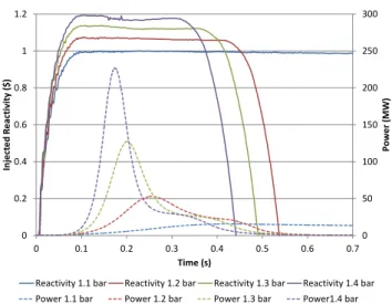
0 50 100 150 200 250 300 0 0.2 0.4 0.6 0.8 1 1.2 0 0.1 0.2 0.3 0.4 0.5 0.6 0.7 P ower (MW) In je ct e d R e ac tiv ity ($) Time (s)
Reactivity 1.1 bar Reactivity 1.2 bar Reactivity 1.3 bar Reactivity 1.4 bar Power 1.1 bar Power 1.2 bar Power 1.3 bar Power1.4 bar
Fig. 13. Effect of small initial pressure variations on measured power transients
from pressure to reactivity.
V. SENSITIVITY STUDY NEAR1 $OF INJECTED REACTIVITY
In this section, we will try to explain the differential between calculation and experiment for low initial pressure transients, based on an uncertainty propagation approach. There is an uncertainty on the pressure measurement of approximately 0.2 % and an uncertainty on 3He reactivity vs.3He density. In cases of low pressure and an injected reactivity close to the effective delayed neutron fraction, the uncertainties are very influent on transient calculation.
A. Experimental approach
During the last commissioning tests, some transients have been carried out with an initial pressure close to 1.2 bar in order to observe the changing physics in this zone. We will compare four transients with close initial pressure (1.1, 1.2, 1.3, 1.4 bar).
We can observe those transients on Fig 13. Below one dollar of injected reactivity, no power pulse is observed, the power increases slower but continues to increase before the rod drop. Above the dollar of injected reactivity, power is increasing until Doppler feedback compensates the injected reactivity.
B. Computational approach
The computational approach consists in propagating the input uncertainties on the power transient calculation. We assume uncertainties on initial pressure, final density, helium reactivity curve, Doppler coefficient model, depressurization model. Those uncertainties are assumed with a standard de-viation of around 5 %. 20 code runs are launched using a Sobol Design of experiments with normal distribution of the input parameters. The computational approach is tested on the 1.3 bar initial pressure case.
We can observe on Fig. 14 the influence of small uncertain-ties on the calculated transient of power. In this area of the
2017-09-20 11:55:52 Time [s] 0 0.05 0.1 0.15 0.2 0.25 0.3 0.35 0.4 Power [MW] 100 200 300 400 500 600
Fig. 14. Uncertainty propagation on the 1.3 bar case with the SPARTE code launched by URANIE
reactivity curve function of the3He pressure, we can assume
that the reactivity model overestimates reality. The experimen-tal power transient (blue) is located near the lower limit of the calculated transients. A good consistency is observed between experiment and calculation when uncertainties are taken into account.
VI. CONCLUSION
The CABRI power transients generated by 3He controlled
depressurization are of two types: “natural” and “structured” and present very complex behavior depending on the kinetics and feedback coefficients. The current DULCINEE multi-physics code, while conservative, presents several assumptions that must be upgraded to enhance safety and operational margins of the CABRI tests. The first goal of the new SPARTE code is to predict at best the “natural” transients. The implementation of surrogate models for the3He density, more relevant than the pressure, for the Doppler coefficient, the axial neutron flux distribution and the neutron life time, based on Best-Estimates calculation and validated against measurements has greatly improved the calculation of those transients. For the prediction of the “structured” transients, we need first to calculate with a good consistency the transients issued from depressurizations of the low flowrate channel. When, the initial pressure is under 5 bar, SPARTE reproduces quite well the measured transients. Over this pressure, the “TOP” effect (described in [8]), affects the reactivity injection speed. We finally observed that the calculation of power transients with injected reactivity near 1 $ is very sensible to the different uncertainties. The analysis of the CABRI commissioning tests recently performed will improve the precision of the reactivity injected by the 3He depressurization.
APPENDIXA NOMENCLATURE Name Definition
P Pressure m mass
B coefficient in s−1 used in depressurization analytical law γ Heat capacity ratio
ρ Reactivity ρD Doppler reactivity
AD Doppler integral coefficient
T Absolute temperature T0 Initial absolute temperature
k Multiplication factor
z Height of insertion of control rods d 3He density
REFERENCES
[1] B. Duc, B. Biard, P. Debias, L. Pantera, J.-P. Hudelot, and F. Rodiac, “Renovation, improvement and experimental validation of the Helium-3 transient rods system for the reactivity injection in the CABRI reactor,” in International Group On Research Reactors, 2014, Bariloche, Argentina, November 17 - 21.
[2] O. Clamens, J. Couybes, J. Lecerf, J.-P. Hudelot, B. Duc, L. Pantera, P. Blaise, and B. Biard, “Analysis of the CABRI power transients -Prediction improvements using a combination of measurements and calculation.” in Proc. Int. Conf. ANIMMA2017, Liege, Jun. 2017. [3] J. Lecerf, Y. Garnier, J.-M. Girard, C. Domergue, L. Gaubert, and
C. Manenc, “Study of the linearity of CABRI experimental chambers during RIA transients,” in Proc. Int. Conf. ANIMMA2017, Liege, Jun. 2017.
[4] J.-P. Hudelot, E. Fontanay, C. Molin, A. Moreau, L. Pantera, J. Lecerf, Y. Garnier, and B. Duc, “CABRI facility: upgrade, refurbishment, recommissioning and experimental capacities,” in Proc. Int. Conf. PHYSOR2016, Sun Valley, USA, 2016.
[5] J. P. Hudelot, J. Lecerf, Y. Garnier, G. Ritter, O. Gueton, A. C. Colombier, F. Rodiac, and C. Domergue, “A complete dosimetry experimental program in support of the core characterization and of the power calibration of the CABRI reactor,” in Advancements in Nuclear Instrumentation Measurement Methods and their Applications (ANIMMA), 2015 4th International Conference on. IEEE, 2015, pp. 1–8. [Online]. Available: http://ieeexplore.ieee.org/abstract/document/ 7465504/
[6] G. Ritter, R. Berre, and L. Pantera, “DULCINEE. Beyond neutron kinetics, a powerful analysis software,” in RRFM IGORR, 2012, prague, Czech Republic, March 18 - 22.
[7] V. Georgenthum, A. Moal, and O. Marchand, “SCANAIR a transient fuel performance code Part two: Assessment of modelling capabilities,” Nuclear Engineering and Design, vol. 280, pp. 172–180, Dec. 2014. [Online]. Available: http://www.sciencedirect.com/science/article/ pii/S0029549314002556
[8] O. Clamens, J. Lecerf, J.-P. Hudelot, B. Duc, T. Cadiou, P. Blaise, and B. Biard, “Assessment of the3He pressure inside the CABRI transient rods - Development of a surrogate model based on measurements and complementary CFD calculations,” in Proc. Int. Conf. ANIMMA2017, Liege, Jun. 2017.
[9] E. Brun, E. Dumonteil, F. Hugot, N. Huot, C. Jouanne, Y. Lee, F. Malvagi, A. Mazzolo, O. Petit, J. Trama, and others, “Overview of TRIPOLI-4 version 7, Continuous-energy Monte Carlo Transport Code,” 2011.
[10] F. Gaudier, “URANIE: The CEA/DEN Uncertainty and Sensitivity platform,” Procedia - Social and Behavioral Sciences, vol. 2, no. 6, pp. 7660–7661, Jan. 2010. [Online]. Available: http://www.sciencedirect. com/science/article/pii/S1877042810013078
[11] O. Clamens, J. Lecerf, B. Duc, J.-P. Hudelot, T. Cadiou, and B. Biard, “Assesment of the CABRI transients power shape by using CFD and point kinetic codes.” in Proc. Int. Conf. PHYSOR2016, Sun Valley, USA, 2016, pp. 1747–1758.
[12] G. Truchet, P. Leconte, A. Santamarina, E. Brun, F. Damian, and A. Zoia, “Computing adjoint-weighted kinetics parameters in Tripoli-4 by the Iterated Fission Probability method,” Annals of Nuclear Energy, vol. 85, pp. 17–26, Nov. 2015. [Online]. Available: http://www.sciencedirect.com/science/article/pii/S030645491500225X