HAL Id: hal-03059013
https://hal.archives-ouvertes.fr/hal-03059013
Submitted on 12 Dec 2020
HAL is a multi-disciplinary open access
archive for the deposit and dissemination of
sci-entific research documents, whether they are
pub-lished or not. The documents may come from
teaching and research institutions in France or
abroad, or from public or private research centers.
L’archive ouverte pluridisciplinaire HAL, est
destinée au dépôt et à la diffusion de documents
scientifiques de niveau recherche, publiés ou non,
émanant des établissements d’enseignement et de
recherche français ou étrangers, des laboratoires
publics ou privés.
comparison, EUROCOM: first results on European-wide
terrestrial carbon fluxes for the period 2006–2015
Guillaume Monteil, Grégoire Broquet, Marko Scholze, Matthew Lang, Ute
Karstens, Christoph Gerbig, Frank-Thomas Koch, Naomi Smith, Rona
Thompson, Ingrid Luijkx, et al.
To cite this version:
Guillaume Monteil, Grégoire Broquet, Marko Scholze, Matthew Lang, Ute Karstens, et al.. The
re-gional European atmospheric transport inversion comparison, EUROCOM: first results on
European-wide terrestrial carbon fluxes for the period 2006–2015. Atmospheric Chemistry and Physics, European
Geosciences Union, 2020, 20 (20), pp.12063-12091. �10.5194/acp-20-12063-2020�. �hal-03059013�
the Creative Commons Attribution 4.0 License.
The regional European atmospheric transport inversion
comparison, EUROCOM: first results on European-wide
terrestrial carbon fluxes for the period 2006–2015
Guillaume Monteil1, Grégoire Broquet2, Marko Scholze1, Matthew Lang2, Ute Karstens3, Christoph Gerbig4, Frank-Thomas Koch5,4, Naomi E. Smith6, Rona L. Thompson7, Ingrid T. Luijkx8, Emily White9, Antoon Meesters10, Philippe Ciais2, Anita L. Ganesan9, Alistair Manning9, Michael Mischurow1, Wouter Peters8,11, Philippe Peylin2, Jerôme Tarniewicz2, Matt Rigby9, Christian Rödenbeck4, Alex Vermeulen12, and Evie M. Walton9
1Dept. of Physical Geography and Ecosystem Science, Lund University, Lund, Sweden 2Laboratoire des Sciences du Climat et de l’Environnement, LSCE/IPSL, CEA-CNRS-UVSQ,
Université Paris-Saclay, Gif-sur-Yvette, France
3ICOS Carbon Portal at Lund University, Lund, Sweden 4Max Planck Institute for Biogeochemistry, Jena, Germany
5Deutscher Wetterdienst, Meteorologisches Observatorium, FEHP, Hohenpeißenberg, Germany 6ICOS Carbon Portal at Wageningen University and Research, Wageningen, the Netherlands 7NILU – Norsk Institutt for Luftforskning, Kjeller, Norway
8Meteorology and Air Quality, Wageningen University and Research, Wageningen, the Netherlands 9University of Bristol, Bristol, BS8 1TS, United Kingdom
10Department of Earth Sciences, Vrije Universiteit Amsterdam, the Netherlands 11Centre for Isotope Research, University of Groningen, Groningen, the Netherlands 12ICOS ERIC – Carbon Portal, Lund, Sweden
Correspondence: Guillaume Monteil (guillaume.monteil@nateko.lu.se) Received: 31 October 2019 – Discussion started: 11 December 2019
Revised: 6 August 2020 – Accepted: 8 September 2020 – Published: 26 October 2020
Abstract. Atmospheric inversions have been used for the past two decades to derive large-scale constraints on the sources and sinks of CO2 into the atmosphere. The
devel-opment of dense in situ surface observation networks, such as ICOS in Europe, enables in theory inversions at a resolu-tion close to the country scale in Europe. This has led to the development of many regional inversion systems capable of assimilating these high-resolution data, in Europe and else-where. The EUROCOM (European atmospheric transport in-version comparison) project is a collaboration between seven European research institutes, which aims at producing a col-lective assessment of the net carbon flux between the terres-trial ecosystems and the atmosphere in Europe for the period 2006–2015. It aims in particular at investigating the capacity of the inversions to deliver consistent flux estimates from the country scale up to the continental scale.
The project participants were provided with a common database of in situ-observed CO2 concentrations (including
the observation sites that are now part of the ICOS network) and were tasked with providing their best estimate of the net terrestrial carbon flux for that period, and for a large domain covering the entire European Union. The inversion systems differ by the transport model, the inversion approach, and the choice of observation and prior constraints, enabling us to widely explore the space of uncertainties.
This paper describes the intercomparison protocol and the participating systems, and it presents the first results from a reference set of inversions, at the continental scale and in four large regions. At the continental scale, the regional in-versions support the assumption that European ecosystems are a relatively small sink (−0.21 ± 0.2 Pg C yr−1). We find that the convergence of the regional inversions at this scale
is not better than that obtained in state-of-the-art global in-versions. However, more robust results are obtained for sub-regions within Europe, and in these areas with dense obser-vational coverage, the objective of delivering robust country-scale flux estimates appears achievable in the near future.
1 Introduction
The carbon budget of Europe has been explored in sev-eral large-scale synthesis studies, such as the CarboEurope-Integrated Project (Schulze et al., 2009) and the REgional Carbon Cycle Assessment and Processes project (RECCAP; Luyssaert et al., 2012), to name a few. Although these have helped refine the knowledge of the European carbon cycle, large uncertainties remain regarding the quantification of the flux between terrestrial ecosystems and the atmosphere, usu-ally quantified as the net ecosystem exchange (NEE), i.e. the sum of emissions (total ecosystem respiration (TER), i.e. autotrophic and heterotrophic respiration) and uptake (gross primary production (GPP), i.e. photosynthesis) of carbon by ecosystems to and from the atmosphere, or alternatively NBP (net biome production), which includes the impact of ecosys-tem disturbances (fires, land use change, etc.). For instance, Luyssaert et al. (2012) report average estimates of European land carbon sink in a −200 to −360 Tg C yr−1 range for the years 2001–2005, depending on the estimation method, and each of these estimates is provided with large uncer-tainties (with 1σ relative unceruncer-tainties of 50 % to 100 %). Confronting the ensemble of results from different synthe-ses, Reuter et al. (2017) report annual land–atmosphere flux ranging from −400±420 up to −1030±470 Tg C yr−1in the 2000s. Beyond the annual long-term budget, the year-to-year annual flux variations are also poorly known (Bastos et al., 2016). In practice, the lack of a robust and precise quantifi-cation of the natural CO2fluxes in Europe limits our ability
to understand the links between the NEE flux and external forcings such as, for example meteorological variability (in-cluding the impact of extreme events like droughts and cold spells) and trends (Ciais et al., 2005; Maignan et al., 2008) or land use change (Naudts et al., 2016), and to forecast the evolution of the land sink in Europe, in the context of global climate change.
Despite the large uncertainties, there is a growing demand from the policy makers and the society in general for more accurate and relevant numbers, such as estimates of the na-tional budgets of CO2fluxes, these demands being reinforced
by the Paris Agreement. For instance, the European Com-mission (under the VERIFY and CHE H2020 projects) is supporting the development of observation-based monitoring systems for estimating CO2fluxes at national to sub-national
scales, with a clear interest in both land ecosystem fluxes and anthropogenic emissions.
Atmospheric transport inversions rely on transport mod-els and statistical methodologies to derive the most likely es-timates of CO2 fluxes given large datasets of observed
at-mospheric CO2 concentrations and prior information
pro-vided in general by ecosystem models. Global inversion sys-tems, using coarse-resolution global transport models (typi-cally > 2◦) have so far been the dominant tool for producing top-down estimates of NEE fluxes. The coordination of the inverse modelling community through intercomparison ex-ercises with ≈ 10 global inverse modelling systems, such as that conducted in the frame of the TRANSCOM and REC-CAP projects (Law et al., 1996; Gurney et al., 2002; Patra et al., 2008; Peylin et al., 2013) have been valuable for under-standing the strengths and weaknesses of global inversions and to characterize the real uncertainty of the different esti-mates. However, despite this long-term effort, global inver-sions remain limited by the coarse resolution of the transport models they rely on, as these do not allow a proper represen-tation of observation sites in regions with complex orogra-phy or nearby large anthropogenic CO2emissions and do not
reproduce the high-resolution spatial variability of the CO2
concentrations that is captured by dense networks.
Regional-scale inversions started to emerge about a decade ago. They rely on mesoscale transport models (at 1◦down to 10 km resolution), capable of better representing the spatial and temporal variability of concentrations observed by dense networks of CO2observations, such as that of the Integrated
Carbon Observation System (ICOS) in Europe. In particular the models should be able to account for CO2fluxes at a scale
that does not smooth too much the hot spots of fossil fuel CO2 emissions in cities and industrial areas. They
demon-strated some potential to solve for continental to subconti-nental budgets at the monthly scale (e.g. Peters et al., 2007; Rödenbeck et al., 2009; Schuh et al., 2010; Gourdji et al., 2012; Broquet et al., 2013; Meesters et al., 2012). However, until recently, there has only been limited efforts to routinely perform regional inversion estimates in Europe (partly ow-ing to the difficult access to long-term time series of quality-controlled CO2data). Most published synthesis studies have
therefore relied on European NEE estimates from global-scale inversions, based on global networks of mostly back-ground sites.
The ICOS atmospheric network (https://icos-atc.lsce.ipsl. fr, last access: 6 August 2020) is now operational and its number of stations should regularly increase from the cur-rent 19 labelled stations towards at least 37 sites, curcur-rently run by 12 and hopefully in the future more European member states. Precursor networks such as those set up in the frame-work of the CarboEurope and GHG-Europe projects (Ra-monet et al., 2010) and the ICOS preparatory phase provide a robust basis for regional inversions during the pre-ICOS decade. The ICOS Carbon Portal (https://www.icos-cp.eu, last access: 6 August 2020) has been set up to support the exchange of observational data and elaborated products re-lated to the carbon cycle, such as CO2fossil fuel flux maps.
In addition to in situ data, the development of satellite obser-vations of CO2following the launch of GOSAT (Kuze et al.,
2009) in 2009 and OCO-2 in 2014 (Crisp et al., 2004) should further densify the observation coverage, in particular with the foreseen European constellation of CO2high-resolution
imagers of the Copernicus Anthropogenic CO2 Monitoring
mission (CO2M; Pinty et al., 2017), starting from 2025. The use of mesoscale transport models will then become neces-sary to fully exploit the potential of these large datasets with observations at high spatial and temporal resolution.
In this context, the EUROCOM (EUROpean atmospheric transport inversion COMparison) project aims to coordinate a European effort to improve the knowledge on the NEE based on an ensemble of long-term European-scale inver-sions (i.e. covering geographical Europe). The project in-volved the participation of seven research groups, which have produced an ensemble of more than (to date) 12 in-versions (including sensitivity experiments), estimating the European NEE for the period 2006–2015 following a pro-tocol described further in this document. The EUROCOM project is therefore one of the first regional inversion inter-comparisons, and the first one at such a scale dedicated to the European NEE.
The first task of the project, to which this paper is ded-icated, is to assess the capacity of regional inversions to robustly estimate European NEE. We focus on key diag-nostics which are typically looked at in synthesis studies, such as the annual and monthly budgets of NEE and the inter-annual variability, for all of Europe and for large re-gions. We use the results from an ensemble of six inversions (one for each participating system), covering a large spec-trum of inversion characteristics (prior constraints, inversion technique, transport models, etc.): PYVAR-CHIMERE (Bro-quet et al., 2011; Fortems-Cheiney et al., 2019, developed at LSCE, France); LUMIA (Lund University Modular Inver-sion Algorithm) (Monteil and Scholze, 2019), developed at Lund University (Sweden) as part of the EUROCOM project; CarboScope-Regional (Kountouris et al., 2018a, b, devel-oped at MPI-Jena, Germany); FLEXINVERT (Thompson and Stohl, 2014, from NILU, Norway); NAME-HB (White et al., 2019b, from the University of Bristol, United King-dom) and CarbonTracker Europe (Peters et al., 2010; van der Laan-Luijkx et al., 2017), from the University of Wagenin-gen, the Netherlands.
The EUROCOM project extends beyond the scope of this paper. Forthcoming studies using a larger ensemble of in-versions (including additional sensitivity experiments) will focus on quantifying and reducing specific aspects of the un-certainty, supporting the improvement of both the regional inversion techniques and the design of the European obser-vation network.
The paper is organized in five sections. Section 2 briefly summarizes the theoretical background behind atmospheric transport inversions. Section 3 details the inversion proto-col, the participating inverse modelling systems and the
in-put products (fluxes and observations) shared within EURO-COM for conducting the inversions. Results are presented in Sect. 4 and then discussed in Sect. 5. Finally, Sect. 6 summa-rizes the paper and provides some remarks on the future of the EUROCOM collaboration, and on regional inverse mod-elling in general.
2 Inverse modelling methodology and terminology The theoretical framework of the atmospheric inverse trans-port modelling has been extensively detailed in past publica-tions (e.g. Enting, 2002; Rayner et al., 2019). Here we only give a brief overview of the basic principles, to facilitate the comprehension of the paper for readers unfamiliar with the approach and to remind of some of the components discussed in detail in Sect. 3.
Bayesian atmospheric inversions rely on the fact that ob-served spatio-temporal gradients of CO2in the atmosphere
reflect the distribution of carbon exchanges between the at-mosphere and other carbon reservoirs. The link between the net CO2exchange at the surface and the CO2concentrations
in the atmosphere is established by a forward atmospheric transport model. A first set of modelled CO2concentrations
(ym=H (x)) is computed at the time and location of real observations (yo), based on a prior assumption of what the CO2 fluxes are (xb). The mismatch between the modelled
and observed concentrations (δy = H (x) − yo) is used to de-rive a correction δx to the prior flux estimate xb. The
pos-terior flux estimate (x = xb+δx) then represents the best
statistical compromise between fitting the observations and limiting the departures to the prior, accounting for the sta-tistical distribution of uncertainties in both observations and prior fluxes.
The vector x is called the control vector. It contains all the parameters that the inversion can adjust. In our case it contains at least the terrestrial ecosystem component of the CO2 fluxes. It can also contain other adjusted parameters
such as bias or boundary concentration terms. The operator H, which establishes the deterministic relationship between a given control vector x and the corresponding modelled con-centrations ymis called the observation operator. It encom-passes the transport model, but also the impact on the mod-elled concentrations of any input of the transport model that is not further adjusted in the inversions (prescribed anthro-pogenic emissions, boundary conditions, etc.).
Following the Bayesian approach and using a classical Gaussian error hypothesis the problem is reduced to finding the posterior control vector xathat minimizes the cost
func-tion J (x), defined as follows:
J (x) =1 2δx TB−1δx | {z } Jb +1 2δy TR−1δy | {z } Jobs . (1)
The prior error covariance matrix B contains a represen-tation of the uncertainties on the prior control vector xband
the error covariance matrix R contains the observational er-ror, which combines the measurement uncertainties (uncer-tainty of the observations y) and the uncertainties associ-ated with the observation operator H : the representation er-ror (due to the comparison of point concentration measure-ments with gridded model concentration) and the model error (uncertainty in non-optimized model parameters, such as the boundary and initial conditions, the non-optimized fluxes, and uncertainty in the model physics). Departing from the prior control vector xbincreases Jb, and improving the fit to
the observations reduces Jobs. B and R modulate the relative
weight of each departure to the prior and to the observations in J .
The exact specifications of B and R affect to a certain ex-tent the outcome of an inversion. For practical reasons, the error covariance matrix for the observations R is usually de-fined as a diagonal matrix with the measurement and model uncertainty (σ ) for each observation site specified on the di-agonal. Potential error correlations between observations are typically dealt with by limiting the density of observations or inflating their individual uncertainties. The diagonal el-ements of the prior error covariance matrix B contains the uncertainties of the prior control parameters (typically here the NEE at the grid scale). The off-diagonal elements, cor-responding to the covariances between uncertainties in dif-ferent control parameters, are difficult to specify because the uncertainties in the NEE estimates have hardly been char-acterized and quantified (Kountouris et al., 2015). They are, however, a critical component of the inversion as they deter-mine how independently from each other the different com-ponents of the control vector can be adjusted. The inversions in this study follow different implementations of this general methodology, listed in Sect. 3.3.2.
The optimal control vector xa can be solved for using
different solution methods. Here we only briefly recall the methods employed by the systems in this study (variational and sequential ensemble approaches, and Markov Chain– Monte Carlo); more information on these methods is given in Rayner et al. (2019) and references therein.
The variational method minimizes J (x) based on iterative gradient descent methods. Efficient implementations of this method rely either on the availability of the adjoint of the transport model or pre-computed transport Jacobian matrices representing the sensitivity of the observation vector to the control vector. The Monte Carlo approach directly samples the cost function, and in the case of the Markov chain–Monte Carlo (MCMC) approach, the samples form a Markov chain; i.e. each sample is not obtained independently, but rather a perturbation of the last previously accepted sample. This lows non-Gaussian PDFs to be used in the inversion and al-lows the specification of uncertainties to be explored in so-called “hierarchical” Bayesian frameworks (Ganesan et al., 2014; Lunt et al., 2016). Finally, the ensemble Kalman
filter-ing (EnKF) directly derives xa following its analytical for-mulation based on the reduction of the dimensions of the problem through the split of the inversion into sequential windows, and based on the computation of the matrices in-volved in the EnKF formulation through an ensemble Monte Carlo approach.
3 Protocol and participating models
Given the overall objective of the study (to assess the ro-bustness of inversion-derived European flux estimates), we deliberately opted for a relatively loose protocol: the partici-pants were requested to use a common set of anthropogenic CO2 emissions (fossil fuel combustion, cement production
and large-scale fires) and to use only atmospheric observa-tions from a common dataset, prepared specifically for the EUROCOM project (Sect. 3.1). They were requested to pro-vide a monthly gridded estimate of the net land–atmosphere CO2exchange (net ecosystem exchange, NEE) over the
pe-riod 2006 to 2015, covering at least the area 15◦W–35◦E by 33–73◦N, at a 0.5◦by 0.5◦spatial resolution (independently of the actual resolution of the inversions).
A set of fluxes (prior NEE, anthropogenic and ocean fluxes) was made available to the modellers through a data repository hosted at the ICOS Carbon Portal, along with the common observation database, but except for the imposed anthropogenic emissions, the participants were essentially free to choose the characteristics of their inversions. In par-ticular they could perform further selections on the observa-tions database (selection of observation sites and selection of observations to use at each site) and choose their prior NEE and ocean flux estimates. The treatment of boundary condi-tions and the precise specification of uncertainties (prior and observation uncertainties) were also left to the modellers.
The inversions in our ensemble are constructed with the aim to maximize the diversity of the systems, and hence to obtain a better estimate of the overall uncertainty of inversion results. A stricter protocol, for example fixing the prior fluxes and the prior uncertainties, would facilitate the interpretation of results but would artificially decrease their spread. Fur-thermore, some parameters should not be prescribed. For in-stance, the observations are selected based on the capacity of the underlying transport model to reproduce them, and the type of boundary condition is also dependent on the transport models, which differ across the systems. It is, however, clear that further steps will be needed, with a stricter protocol, to fully understand the specific causes of the discrepancies that were obtained.
3.1 Common atmospheric observation database A comprehensive dataset of atmospheric CO2concentration
observations in Europe was compiled as input for the inver-sion systems, on the basis of the GLOBALVIEWplus v3.2
Observation Package (ObsPack), a product compiled and co-ordinated at NOAA’s Earth System Research Lab together with the ICOS Carbon Portal (Cooperative Global Atmo-spheric Data Integration Project, 2017). The dataset was further extended by including measurements that had been collected in several national and EU-funded projects, like CarboEurope-IP and GHG-Europe, and during the prepara-tory phase of the Integrated Carbon Observation System (ICOS) Research Infrastructure. Finally, for two stations, the data were obtained from the World Data Center for Green-house Gases (https://gaw.kishou.go.jp/, last access: 6 August 2020).
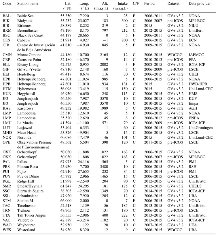
Compared to the original GLOBALVIEWplus product, we added time series from nine measurement stations and partly complemented time series at two stations. The datasets were harmonized with respect to format and sampling interval and provided in the ObsPack format (Masarie et al., 2014). The original datasets and data providers of the time series are re-ported in Table 1, and the locations of the observation sites are also shown in Fig. 1.
The majority of sites (35 out of 39) sample concentrations continuously (i.e. hourly or more frequently); 18 sites are tall towers (intake height > 50 m), some with observations avail-able at different levels, in which case only the upper level was used (as it is more difficult for the transport models to represent concentration gradients close to the ground).
The modellers were free to refine the observation selection according to the ability of their inversion systems to simulate specific stations, and in particular to use their preferred ap-proach to select data within a day (i.e. use of all the observa-tions within a time frame or use of an average of the obser-vations, etc.). The precise observation selection approaches are discussed further in Sect. 3.3.3, and a full comparison of the observation assimilated by each system is provided in Figs. S1 and S2 in the Supplement.
3.2 Prior and prescribed CO2fluxes
All groups split the total surface–atmosphere CO2 flux in
three or four categories: biosphere (NEE, optimized), ocean (sea–atmosphere CO2exchanges, prescribed or optimized),
anthropogenic (prescribed) and biomass burning (prescribed, used by LUMIA and FLEXINVERT+).
Note that we use the term NEE (sum of photosynthesis and ecosystem respiration) for the posterior fluxes over land throughout the paper, because this is what the prior flux esti-mates from the terrestrial ecosystem models represent. How-ever, strictly speaking, the inversions optimize the flux that is not explained by the prescribed anthropogenic (and some-times ocean) fluxes. This includes the effect of ecosystem disturbances (land use, land management, biotic effects) but also projection of errors in the prescribed fluxes.
Atmospheric inversions usually rely on NEE simulations from terrestrial ecosystem models to provide the prior value of the NEE component of the control vector (as defined above in Sect. 2). Within EUROCOM four different simulations of gross (GPP and ecosystem respiration) and net (NEE) ter-restrial biosphere fluxes were included: three from process-based models (ORCHIDEE, LPJ-GUESS and SiBCASA), and one from a diagnostic model (VPRM). Two of the four models (ORCHIDEE and LPJ-GUESS) are providing input for the Global Carbon Project annual global CO2assessment
(Le Quéré et al., 2018).
– ORCHIDEE (used by PYVAR-CHIMERE, FLEXIN-VERT+ and NAME-HB): ORCHIDEE (Krinner et al., 2005) computes carbon, water and energy fluxes be-tween the land surface and the atmosphere and within the soil–plant continuum. The model computes the gross primary productivity with the assimilation of car-bon based on Farquhar et al. (1980) for C3 plants.
Land cover changes (including deforestation, regrowth and cropland dynamic) were prescribed using annual land cover maps derived from the harmonized land use dataset (Hurtt et al., 2011) combined with the ESA-CCI land cover products. The ORCHIDEE simulation used here has been produced at a global, 0.5◦resolution with 3-hourly output.
– LPJ-GUESS (used by LUMIA): LPJ-GUESS (Smith et al., 2014) combines process-based descriptions of terrestrial ecosystem structure (vegetation composition, biomass and height) and function (energy absorption, carbon and nitrogen cycling). Vegetation is dynamically simulated as a series of replicate patches, in which in-dividuals of each simulated plant functional type (or species) compete for the available resources of light and water, as prescribed by the climate data. LPJ-GUESS includes an interactive nitrogen cycle. The simulation used here is forced using the WFDEI meteorological dataset (Weedon et al., 2014) and produces a 3-hourly output of gross and net carbon fluxes at a 0.5◦ horizon-tal resolution.
– SiBCASA (used by CTE): SiBCASA (Schaefer et al., 2008) combines the parameterization of the Simple Bio-sphere model (SiB) with the biogeochemistry of the Carnegie–Ames–Stanford approach (CASA) calculat-ing the exchange of water, carbon and energy between 25 soil layers, plants and the atmosphere. The rate of photosynthesis is found using the Ball–Berry–Woodrow model of stomatal conductance (Ball et al., 1987), and C3and C4vegetation types are treated separately in the
kinetic enzyme model of Farquhar et al. (1980). The simulation used here is forced using meteorological in-puts from ERA-Interim and run with a 10 min time step
Table 1. Observation sites used in the inversions. Datasets with in situ continuous (C) as well as flask (F) measurements were taken from GLOBALVIEWplus ObsPack, WDCGG, and the EU-funded projects CarboEurope-IP, GHG-Europe and ICOS preparatory phase (all indi-cated as pre-ICOS).
Code Station name Lat. Long. Alt. Intake C/F Period Dataset Data provider (◦N) (◦E) (m a.s.l.) (m a.g.l.)
BAL Baltic Sea 55.350 17.220 3 25 F 2006–2011 GV+ v3.2 NOAA BIK Białystok 53.232 23.027 183 300 C 2006–2007 pre-ICOS MPI-BGC BIR Birkenes 58.389 8.252 219 2 C 2015 GV+ v3.2 NILU BRM Beromünster 47.190 8.175 797 212 C 2012–2015 GV+ v3.2 Uni.Bern BSC Black Sea Coast 44.178 28.665 0 5 F 2006–2011 GV+ v3.2 NOAA CES Cabauw 51.971 4.927 −1 200 C 2006–2015 GV+ v3.2 ECN CIB Centro de Investigación 41.810 −4.930 845 5 F 2009–2015 GV+ v3.2 NOAA
de la Baja Atmósfera
CMN Monte Cimone 44.180 10.700 2165 12 C 2006–2015 WDCGG IAFMCC CRP Carnsore Point 52.180 −6.370 9 14 C 2010–2013 pre-ICOS EPA ELL Estany Llong 42.575 0.955 2002 3 F 2008–2015 GV+ v3.2 ICTA-ICP GIF Gif-sur-Yvette 48.710 2.148 160 7 C 2006–2009 pre-ICOS LSCE HEI Heidelberg 49.417 8.674 116 30 C 2006–2015 GV+ v3.2 UHEI HPB Hohenpeißenberg 47.801 11.024 985 5 F 2006–2015 GV+ v3.2 NOAA HPB Hohenpeißenberg 47.801 11.010 934 131 C 2015 GV+ v3.2 DWD-HPB HTM Hyltemossa 56.098 13.419 115 150 C 2015 GV+ v3.2 Uni.Lund-CEC HUN Hegyhátsál 46.950 16.650 248 115 C 2006–2015 GV+ v3.2 HMS JFJ Jungfraujoch 46.550 7.987 3570 10 C 2006–2015 GV+ v3.2 KUP JFJ Jungfraujoch 46.550 7.987 3570 10 C 2010–2015 GV+ v3.2 Empa KAS Kasprowy 49.232 19.982 1989 5 C 2006–2015 GV+ v3.2 AGH LMP Lampedusa 35.510 12.610 45 5 F 2006–2015 GV+ v3.2 NOAA LMP Lampedusa 35.520 12.620 45 8 C 2006–2012 pre-ICOS ENEA LMU La Muela 41.594 −1.100 571 79 C 2006–2009 pre-ICOS ICTA-ICP LUT Lutjewad 53.404 6.353 1 60 C 2006–2015 GV+ v3.2 Uni.Groningen MHD Mace Head 53.326 −9.904 5 15 C 2006–2015 GV+ v3.2 LSCE NOR Norunda 60.086 17.479 46 101 C 2015 GV+ v3.2 Uni.Lund-CEC OPE Observatoire Pérenne 48.562 5.504 390 120 C 2011–2015 pre-ICOS LSCE
de l’Environnement
OXK Ochsenkopf 50.030 11.808 1022 163 F 2006–2015 GV+ v3.2 NOAA OXK Ochsenkopf 50.030 11.808 1022 163 C 2006–2007 pre-ICOS MPI-BGC PAL Pallas 67.973 24.116 565 5 C 2006–2015 GV+ v3.2 FMI PRS Plateau Rosa 45.930 7.700 3480 10 C 2006–2015 GV+ v3.2 RSE PUI Pujio 62.910 27.655 232 84 C 2011–2014 pre-ICOS FMI PUY Puy de Dôme 45.772 2.966 1465 15 C 2006–2015 GV+ v3.2 LSCE RGL Ridge Hill 51.998 −2.540 204 90 C 2012–2015 GV+ v3.2 Uni.Bristol SMR Smear/Hyytiälä 61.847 24.295 181 125 C 2012–2015 GV+ v3.2 UHELS SSC Sierra de Segura 38.303 −2.590 1349 20 C 2014–2015 GV+ v3.2 ICTA-ICP SSL Schauinsland 47.920 7.920 1205 12 C 2006–2015 GV+ v3.2 UBA STM Station M 66.000 2.000 0 7 F 2006–2015 GV+ v3.2 NOAA TAC Tacolneston 52.518 1.139 56 185 C 2013–2015 GV+ v3.2 Uni.Bristol TRN Traînou 47.965 2.112 131 180 C 2006–2015 pre-ICOS LSCE TTA Tall Tower Angus 56.555 −2.986 400 222 C 2013–2015 GV+ v3.2 Uni.Bristol VAC Valderejo 42.879 −3.214 1102 20 C 2013–2015 GV+ v3.2 ICTA-ICP WAO Weybourne 52.950 1.122 20 10 C 2007–2015 GV+ v3.2 UEA WES Westerland 54.930 8.320 12 9 C 2006–2015 WDCGG UBA
and a spatial resolution of 1◦×1◦. The actual temporal resolution used in the inversion is 3 h.
– VPRM (used by CarboScope-Regional): VPRM (Ma-hadevan et al., 2008) calculates photosynthetic
up-take based on a light-use efficiency approach and temperature-dependent ecosystem respiration. It uses ECMWF operational meteorological data for radiation and temperature, the SYNMAP land cover classifica-tion (Jung et al., 2006), and MODIS-derived EVI
(en-Figure 1. EUROCOM domain (pale blue grid with the 0.5◦resolution) and location of the observation sites. The size of the dots is propor-tional to the number of months with at least one observation available (in the common observation database, not all observations are used in the inversions), and the colour map shows the altitude of the sites (height above ground + sampling height). The four regions used in the analysis are also represented: western Europe (green), southern Europe (blue), central Europe (yellow) and northern Europe (grey).
hanced vegetation index) and LSWI (land surface water index). Model parameters were optimized for Europe using eddy covariance measurements made during 2007 from 47 sites (Kountouris et al., 2015). The VPRM sim-ulation used here has been produced at a 0.25◦spatial and hourly temporal resolution.
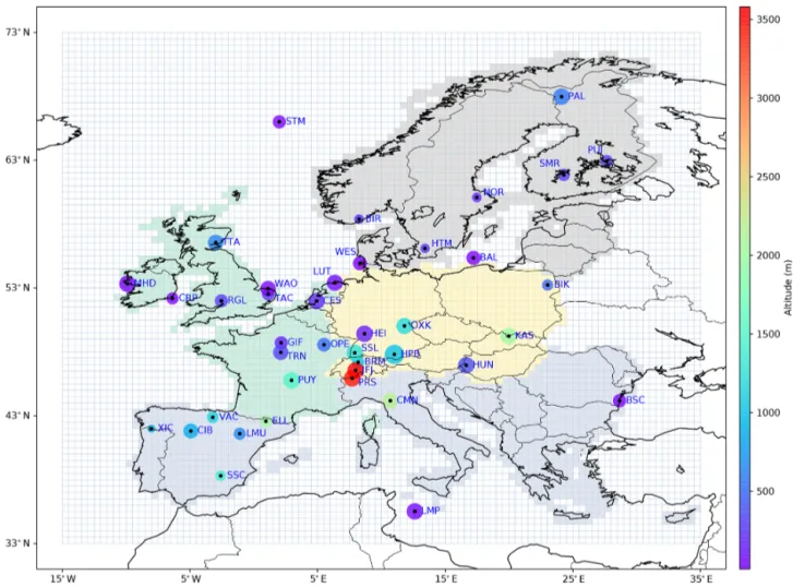
The mean seasonal cycle and the inter-annual variabil-ity of these NEE simulations are shown in Fig. 2. Among the notable features is the annual mean NEE of VPRM, which is much lower (≈ −1.1 Pg C yr−1) than that of the three other models (ranging from −0.1 to −0.4 Pg C yr−1). VPRM is known to produce an uptake that is too large (Oney et al., 2017), which can be explained by the opti-mization of this diagnostic model against flux measurements from one year. The year-to-year variations of the annual budget are significant (≈ 0.1 Pg C yr−1) but not always in phase between the four models. For the mean seasonal cy-cle, the peak-to-peak amplitude differs significantly between the models, with the smallest amplitude obtained with
LPJ-GUESS (around 0.4 Pg C per month) and the largest with ORCHIDEE (around 0.8 Pg C per month). Another visible feature is the phasing of the seasonal cycle in LPJ-GUESS, with an earlier CO2peak uptake than the other three models
(May versus June) and a peak release in August. This phase difference has already been described by Peng et al. (2015). 3.2.2 Anthropogenic emissions
The anthropogenic emissions from combustion of fossil fu-els and biofufu-els and from cement production are based on a pre-release of the EDGARv4.3 inventory for the base year 2010 (Janssens-Maenhout et al., 2019) and were provided as a 0.5◦, hourly resolution product. This specific dataset in-cludes additional information on the fuel mix per emission sector (Janssens-Maenhout, personal communication, 2017) and thus allows for a temporal scaling of the gridded an-nual emissions for individual years (2006–2015) according to year-to-year changes of fuel consumption data at national level (BP, 2016), following the approach of Steinbach et al.
Figure 2. Seasonal cycle (a) and inter-annual variability (b) of the prior NEE (coloured lines/shading) and prescribed anthropogenic flux (black) used in the inversions, for geographical Europe (see definition in Sect. 3). The solid lines in the upper plot represents the mean seasonal cycle over the 10 years of the study, while the shaded envelopes show the minimum and maximum values over the same period.
(2011). A further temporal disaggregation into hourly emis-sions is based on specific temporal factors (seasonal, weekly and daily cycles) for different emission sectors (Denier van der Gon et al., 2011). The seasonality and inter-annual vari-ability of this anthropogenic emissions prior are also reported in Fig. 2 (in black).
Agricultural waste burning is already included in the ver-sion of the EDGAR v4.3 anthropogenic emisver-sion inven-tory that we are using. Also, large-scale biomass burn-ing emissions are negligible in Europe (of the order of 0.01 Pg C yr−1), and therefore we decided that no extra biomass burning emission dataset should be used in the in-versions. Nevertheless, two models (LUMIA and FLEXIN-VERT) included a prescribed biomass burning source, based on the Global Fire Emission Database v4 (Giglio et al., 2013).
3.2.3 Ocean fluxes
The role of the ocean flux in causing spatial CO2
gradi-ents between stations at the European scale is very mi-nor in regard to the magnitude of other fluxes (below −0.1 Pg C yr−1). Therefore modelling groups were free to choose which ocean fluxes to use.
Two groups (LUMIA and FLEXINVERT+) used ocean fluxes from the CarboScope surface-ocean pCO2
interpola-tion (oc_v1.6 and oc_v1.4 respectively) (Rödenbeck et al., 2013). The CarboScope interpolation provides temporally and spatially resolved estimates of the global sea–air CO2
flux. Fluxes are estimated by fitting a simple data-driven diagnostic model of ocean mixed-layer biogeochemistry to surface-ocean CO2 partial pressure data from the SOCAT
database. NAME-HB used a climatological prior from Taka-hashi et al. (2009), which is based on a climatology of surface ocean pCO2constructed using measurements taken between
1970 and 2008. The CarboScope-Regional inversion used an ocean flux estimate taken from the Mikaloff Fletcher et al. (2007) global oceanic air–sea CO2 inversion and
Carbon-Tracker Europe optimized prior fluxes from the ocean inver-sion of Jacobson et al. (2007). Finally, PYVAR-CHIMERE used a null ocean prior but allowed the inversion to adjust it.
3.3 Inversion systems
The six inversion systems encompass a wide range of mesoscale regional transport models (with both Lagrangian and Eulerian models) and of approaches for the inversion (variational, ensemble and MCMC methods). The systems also differ by the definition of the boundary conditions, the selection of the observations to be assimilated, the definition of the control vector and the parameterization of uncertainty covariance matrices. Table 2 presents an overview of the par-ticipating systems characteristics.
3.3.1 Transport models and boundary conditions The six systems cover a diversity of models and model set-ups. Two systems (PYVAR-CHIMERE and CTE) rely on Eu-lerian transport models. The atmosphere is represented by a 3D grid (latitude, longitude and height). The CO2
concen-tration is defined at each grid point and is altered at each time step by the CO2 sources and sinks (i.e. the inversion
control vector) in the surface layer, and by the air mass ex-changes between the grid cells (at all layers). The other sys-tems (LUMIA, FLEXINVERT, CarboScope-Regional and NAME-HB) all rely on Lagrangian transport models. In these systems, a Lagrangian transport model is used to compute, for each observation, a response function (footprint), i.e. a Jacobian matrix containing the sensitivity of the observed concentration to surface fluxes. The change in CO2
T able 2. Ov ervie w of the in v erse modelling systems and configuration of the in v ersions. In v ersion system PYV AR-CHIMERE (LSCE) LUMIA (Lund Uni v ersity) FLEXINVER T (NILU) CarboScope-Re gional (MPI-BGC-Jena) CarbonT rack er Europe (WUR) N AME-HB (Uni. Bristol) Reference Broquet et al. (2011 ), F ortems-Cheine y et al. (2019) Monteil and Scholze (2019) Thompson and Stohl (2014) K ountouris et al. (2018a ) Peters et al. (2010 ), v an der Laan-Luijkx et al. (2017 ) White et al. (2019b ) Method V ariational V ariational V ariational V ariational EnKF MCMC T ransport model CHIMERE (Eulerian) FLEXP AR T (Lagrangian) FLEXP AR T (Lagrangian) STIL T (Lagrangian) TM 5 (Eulerian) N AME (Lagrangian) Meteorological forcing ECMWF operational forecasts ECMWF ERA-Interim reanalysis ECMWF operational forecasts ECMWF operational forecasts ECMWF ERA-Interim reanalysis UK Met Of fice’ s Unified Model (Cullen , 1993 )
Background/ boundary condition
Prescribed at domain edge from a CAMS LMDZ in v ersion Prescribed at obs. location from a TM5-4D V AR in v ersion interpolation of NO AA data + transport of prescribed flux es outside the EUR OCOM domain Prescribed at obs. location from a global CarboScope in v ersion None (global in v ersion) Optimized at domain edge, from a MOZAR T simulation prior T ransport and in v ersion domain 31.5 to 74 ◦N; 15.5 ◦W to 35 ◦E 33 to 73 ◦N; 15 ◦W to 35 ◦E Global transport, in v ersion on a 30–75 ◦N, − 15–35 ◦E domain 33 to 73 ◦N, 15 ◦W to 35 ◦E Global, zoom o v er Europe (12–66 ◦N, 21 ◦W –39 ◦E) 10.729 to 79.057 ◦N; 97.9 ◦W to 39.38 ◦E In v ersion spatial resolution 0 .5 ◦× 0 .5 ◦ 0 .5 ◦× 0 .5 ◦ PFTs × countries 0 .5 ◦× 0 .5 ◦ 1 ◦× 1 ◦o v er Europe, 3 ◦× 2 ◦globally Lar ge re gions × PFTs In v ersion temporal resolution 6 h 1 month 12 h 3 h W eekly V ariable (max 1 d) Prior estimate of NEE ORCHIDEE LPJ-GUESS ORCHIDEE VPRM SiBCASA ORCHIDEE Correlation (spatial, temporal) scales of the prior uncertainty 200 km, 1 month 200 km, 1 month No spatial correlation between PFT/country re gions, 1 month 100 km, 1 month 200 km with no correlation between dif ferent PFTs, 5 weeks No correlations (lar ge re gions) Ocean flux es P art of the control v ector (6 h and 0.5 ◦resolution), null prior Prescribed (Rödenbeck et al. , 2013 ) Prescribed (Rödenbeck et al. , 2013 ) Prescribed (Mikalof f Fletcher et al. , 2007) Optimized (Jacobson et al. , 2007 ) Prescribed (Takahashi et al. , 2009 ) Observ ation selection ∗ 12:00 to 18:00 L T belo w 1000 m a.s.l. and 00:00 to 06:00 L T abo v e 11:00 to 15:00 L T lo w altitude, 23:00 to 03:00 L T high altitude 12:00 to 16:00 L T belo w 1000 m a.s.l. and 00:00 to 04:00 L T abo v e 11:00 to 16:00 UTC lo w altitude and 23:00 to 04:00 UTC at mountain stations 11:00 to 15:00 L T lo w altitude, 23:00 to 03:00 L T at high altitude Based on transport model performance ∗ The classification of lo w and high altitude v aries on a case-by-case basis in some systems; see Fig. S2 for more information.
product of each footprint by the corresponding (slice of) the flux vector.
Beyond the Lagrangian/Eulerian distinction, the models differ by the underlying meteorological data used, and by the domain extent:
– The CHIMERE model (used in the PYVAR-CHIMERE system) is a regional Eulerian Chemistry transport model (Menut et al., 2013), forced with ECMWF op-erational forecasts. The simulations are performed at a horizontal resolution of 0.5◦ and with 29 vertical lev-els up to 300 hPa, for the exact EUROCOM domain (as described at the beginning of Sect. 3).
– The CTE inversion relies on the global Eulerian trans-port model TM5 (Huijnen et al., 2010), driven by air mass transport from the ECMWF ERA-Interim reanal-ysis. TM5 is here run at a global resolution of 3◦×2◦, with a nested 1◦×1◦ zoom over Europe (12–66◦N, 21◦W–39◦E), and 25 vertical sigma-pressure levels. – The CarboScope-Regional system (Kountouris et al.,
2018a) relies on footprints from the STILT model (Lin et al., 2003). STILT footprints are computed for the exact EUROCOM domain, at a horizontal resolution of 0.25◦, and at hourly temporal resolution, and they cover a period of 10 d prior to each observation. STILT is driven by short-term forecasts of the ECMWF-IFS model at 0.25◦ resolution. The surface layer (up to which surface fluxes are mixed instantaneously) is de-fined as half the height of the planetary boundary layer, at any given time.
– In LUMIA, footprints covering the EUROCOM do-main at a 0.5◦, 3-hourly resolution were generated with the FLEXPART 10.0 model (Pisso et al., 2019), driven by ECMWF ERA-Interim meteorology. The footprints cover a period of 7 d prior to each observation and the surface layer is defined as the atmosphere below 100 m a.g.l.
– The FLEXINVERT inversion (Thompson and Stohl, 2014) also relies on footprints from the FLEXPART model, but driven by ECMWF operational forecasts. In contrast to CarboScope-Regional and LUMIA, the foot-prints are computed globally, on a 0.5◦hourly grid, and cover a period of 5 d before each observation.
– The NAME-HB system (White et al., 2019b) uses foot-prints from the NAME Lagrangian particle dispersion model. NAME is driven by 3-hourly meteorology from the UK Met Office’s Unified Model (Cullen, 1993), at a spatial resolution which changes in time of 0.233◦ lat-itude by 0.352◦longitude before mid-2014. The foot-prints are defined on a large regional domain, ranging from 10.729◦N, 97.9◦W to 79.057◦N, 39.38◦E with a
spatial resolution of 0.233◦×0.352◦(it covers the east-ern half of North America, Europe and the northeast-ern half of Africa). The footprints are computed for a period of 30 d before each observation, at a 2-hourly temporal res-olution in the first 24 h, and the remaining 29 d are inte-grated. The surface layer is defined as the layer below a height of 40 m.
Except for CTE which relies on a global model (although it runs at a very coarse resolution outside Europe), and all the other systems need boundary conditions (also called back-ground concentrations), which represent the contribution of fluxes outside the space–time domain of the simulation:
– In PYVAR-CHIMERE and in NAME-HB, the back-ground concentration (BCs) correspond to the trans-port of a boundary condition defined at the edge of the domain, by the transport model used in the inversion. In PYVAR-CHIMERE, the boundary condition is pro-vided by a CAMS global inversion (Chevallier et al., 2010) and in NAME-HB it is derived from a global CO2
simulation with the MOZART transport model (Palmer et al., 2018) (sampled at the time when and location where the NAME trajectories leave the NAME domain). – CarboScope Regional and LUMIA both implement the two-step approach described in Rödenbeck et al. (2009). In short, the background concentrations correspond to the transport to the observation points of a boundary condition, taken from a global, coarse-resolution in-version, by the global transport model used in that global inversion. CarboScope-Regional relies on TM3 for its global inversion, and LUMIA relies on the TM5-4DVAR model.
– In FLEXINVERT, the footprints are global, therefore the background (from the perspective of the transport model) results only from the transport to the observa-tion sites of the initial CO2 distribution (i.e. the CO2
distribution at the start of the period covered by each footprint). This initial concentration is calculated as a weighted average of a global CO2distribution sampled
where and when the FLEXPART trajectories are ter-minated, and this global CO2 distribution is based on
a bivariate interpolation of observed CO2 mixing
ra-tios from NOAA sites globally, with monthly resolved fields. Note that for this system, the domain of the trans-port model is larger than that of the inversion itself. The boundary conditions are specific to each system: from a technical point of view, the differences in domain extent and in the types of couplings with the boundary or background would make it hard to impose a common BC, but also, the boundary condition is an uncertain term: allowing a diversity of implementations is a way to maximize the exploration of the uncertainties in our intercomparison.
Four out of the six systems (PYVAR-CHIMERE, LUMIA, CarboScope-Regional and FLEXINVERT+) implement a variational inversion approach, in which the minimum of the cost function J (x) (Eq. 1) is searched for iteratively. The CTE inversion (Peters et al., 2007; van der Laan-Luijkx et al., 2017) employs an ensemble Kalman smoother with 150 members and a 5-week fixed-lag assimilation window. The NAME-HB inversion uses the MCMC method (Rigby et al., 2011; Ganesan et al., 2014; Lunt et al., 2016; White et al., 2019b). In short, this method samples the parameter space, and proposals for parameter values are accepted or re-jected according to some rules based on the likelihood of the proposal.
Regardless of the inversion technique used, all the groups were asked to provide optimized NEE fluxes at a monthly, 0.5◦ resolution on the EUROCOM domain. However, the precise control vector optimized in some of the inversions differ from this requested product:
– In PYVAR-CHIMERE, the NEE is optimized at a 6-hourly resolution on each grid cell (on the standard EU-ROCOM grid), starting from a prior NEE estimate from the ORCHIDEE model (See Sect. 3.2.1). In addition, the inversion also adjusts the ocean flux estimate, start-ing from a null prior. The prior uncertainty for each control vector element is proportional to the respira-tion in the corresponding grid cell (according to the same ORCHIDEE simulation) and further scaled to ob-tain an average uncerob-tainty at the 0.5◦and 1 d scale of 2.27 µmol CO2m−2s−1(after Kountouris et al., 2018b).
– The LUMIA inversion controls the NEE fluxes monthly, on the standard EUROCOM grid, starting from prior NEE from the LPJ-GUESS model. The prior uncer-tainty is set to 50 % of the prior control vector (i.e. the prior NEE), with a minimum uncertainty set to 1 % of the grid point with the largest uncertainty, to avoid zero-uncertainty when NEE is close to zero. The decadal inversion was decomposed in 10 14-month inversions, from which the first and last month were not used. – In the CarboScope-Regional system, the NEE fluxes are
optimized every 3 h at a 0.5◦resolution in the EURO-COM domain, based on a prior NEE estimate from the VPRM model. The uncertainty of the prior NEE is set to a uniform value of 2.27 µmol CO2m−2s−1, using a
spa-tial error structure with a hyperbolic correlation shape. The set-up is identical to the “nBVH/” case in Koun-touris et al. (2018a). The decadal inversion period was divided into three periods (2006–2007, 2008–2011 and 2012–2015).
– FLEXINVERT+ controls the NEE per country × plant functional type (116 control variables per time step
across Europe, with PFTs based on those in the CLM model). The fluxes are optimized for 6-hourly periods (00:00–06:00, 06:00–12:00, 12:00–18:00, 18:00–00:00 local time, LT), averaged over 5 d. The prior NEE flux is based on the ORCHIDEE simulation described in Sect. 3.2.1, and the uncertainties are set proportional to this prior NEE. The transport model in FLEXINVERT+ is global, therefore the flux estimates used in the inver-sions are defined over the entire globe. However, the in-version only adjusts NEE within the EUROCOM do-main.
– In NAME-HB, the domain of NAME has been split into eight boxes: four “background” boxes outside the EU-ROCOM domain, and four “foreground” boxes within the EUROCOM domain. The latter were further di-vided based on a PFT map used in the JULES veg-etation model (Still et al., 2009), which includes six PFTs. The inversion optimizes separately the gross pri-mary production (GPP, i.e. the uptake of carbon by plants) and the heterotrophic respiration (TER, with NEE = GPP + TER). The flux components are opti-mized at a variable temporal resolution, with a maxi-mum resolution of 1 d (see White et al., 2019b, for fur-ther details). The oceanic flux is prescribed (based on the Takahashi et al., 2009, climatological pCO2
esti-mate), but the background concentrations are part of the control vector and are therefore adjusted during the in-version. Therefore, there are 56 elements in the control vector, 4 elements to optimize the background concen-trations, 4 × 2 elements to optimize the “background” regions for each of GPP and TER, 4 × 5 elements for the PFT regions for GPP (as one of the six PFTs is not applicable to GPP) and finally 4 × 6 elements for the PFT regions for TER. The uncertainties are set to 100 % of the prior for GPP and TER, and to 3 % of the initial value for the background terms.
– in CTE, the NEE and ocean fluxes are optimized glob-ally on a weekly time resolution in a 5-week lagged win-dow. The global domain is split into 11 TRANSCOM regions, which are further decomposed in ecoregions corresponding to 19 ecosystem types. The fluxes are op-timized on 1◦×1◦ resolution for the Northern Hemi-sphere land regions, and by ecoregion and ocean region for the rest of the world. The prior NEE is taken from the SiBCASA simulation described in Sect. 3.2.1, and the prior oceanic flux is based on Jacobson et al. (2007). In the three systems that optimize NEE at the pixel scale (LUMIA, PYVAR-CHIMERE and CarboScope-Regional), the spatial resolution of the control vector is in practice fur-ther limited by the use of distance-based spatial and tempo-ral covariances in the flux covariance matrices (B in Eq. 1), which in effect smoothes the results by preventing the in-version from adjusting neighbouring pixels totally
indepen-dently. The values of 100 km (CarboScope-Regional) and 200 km (PYVAR-CHIMERE and LUMIA) used for the spa-tial covariance lengths correspond well to the diagnostics of comparisons between the ecosystem simulations and flux eddy covariance measurements (Kountouris et al., 2018a). These systems and FLEXINVERT+ also assume temporal error covariances of 1 month at each grid cell.
The NAME-HB and FLEXINVERT+ inversions only con-trol a limited number of PFTs in each region, which means that pixels in the same region and corresponding to the same PFT have a correlation coefficient of 1. Finally, CTE follows an intermediate approach. The flux uncertainties of Northern Hemisphere land pixels within a same ecore-gion are correlated with a variable spatial covariance length to reflect the observation network density (200 km in Eu-rope), and the uncertainties of grid boxes corresponding to different ecoregions are assumed to be uncorrelated. For the rest of the world, the uncertainties are coupled within each TRANSCOM region, decreasing exponentially with distance. The chosen prior standard deviation is 80 % on land parameters and 40 % on ocean parameters (van der Laan-Luijkx et al., 2017).
3.3.3 Observation vectors and errors
All the inversions use observations from the stations listed in Table 1. Each participant was, however, free to refine their selection of observations (both in terms of the number of sites assimilated and of data selection at each site) to adapt it to the skills of their own inversion system. In practice, five of the six inversions used data from nearly all the observation sites. NAME-HB used only a restricted list of 15 sites (see Fig. S1).
Most of the systems assimilate instantaneous or 1 h av-erages of the measurements, taken, when there are several vertical levels of measurements, at the top level of the sta-tions, as it is the least sensitive to very local surface fluxes. NAME-HB assimilates 2-hourly observations (average of the observed concentrations in each 2-hourly interval). Due to the traditional limitations of transport models in terms of representation of the orography and simulation of the ver-tical mixing (Broquet et al., 2011), most of the systems use observations at low-altitude sites during the afternoon only, and observations at high-altitude sites during night-time only (vertical gradients of CO2near to the surface are notoriously
difficult to simulate accurately, so observations when the ver-tical gradients are expected to be lower are preferred.)
– PYVAR-CHIMERE assimilates 1 h averages of the continuous or flask measurements over specific time windows that depend on the altitude of the stations above sea level. The selection window is 12:00– 18:00 UTC time for stations below 1000 m a.s.l. and 00:00–06:00 LT for stations above 1000 m a.s.l. (follow-ing the analysis and choices by Broquet et al., 2011). The observation errors are set up as a function of
sta-tions, of the height of the station level above the ground and of the season, following the estimates by Broquet et al. (2011, 2013), based on comparison of simulations and measurements of radon. Their standard deviation for the 1 h averages ranges from 3 to 17 ppm.
– In LUMIA, observations from sites with con-tinuous observations are selected based on the ‘‘dataset_time_window_utc” flag in the metadata of the observation files. That corresponds, for most sites, to a 11:00 to 15:00 UTC time range, and to a 23:00 to 03:00 UTC time range for mountain sites. At sites with only flask observations, all samples were used. The observation uncertainties are set as the quadratic sum of the measurement uncertainties, of the uncertainty associated with the foreground transport model (i.e. FLEXPART) and to the background con-centrations. The measurement uncertainties are taken from the data files when available, and a minimum un-certainty of 0.3 ppm is enforced. Foreground transport model uncertainties are computed by performing two similar forward model runs, with TM5 and LUMIA (i.e. FLEXPART + background concentrations from TM5), configured such that the only difference is the model used to compute the transport within the EUROCOM domain (since the two models run at very different resolutions, this provides a reasonable proxy for the representation error). The uncertainties on the background concentrations are set as the standard deviation of the vertical profile of background CO2
concentrations around each observation (see Monteil and Scholze, 2019, for details about the approach). Finally, a minimum value of 1 ppm was enforced for the combined uncertainty. On average, the combined uncertainty is of the order of 2 ppm (with site averages ranging from 1.02 for MHD to 4 ppm for PUI), but for individual observations it can be as high as 30 ppm. – CarboScope-Regional assimilates observations,
be-tween 11:00 and 16:00 UTC for tall-towers, ground-based or coastal stations, and from 23:00 to 04:00 UTC for mountain stations (the time intervals refer to the be-ginning of the observation hour). A base representation error of 1.5 ppm was assumed for tall towers, coastal and mountain. For ground based continental sites it was raised to 2.0 ppm, and to 4 ppm for Heidelberg, which is in a urban environment. For sites that provide hourly observations, an error inflation was applied (e.g. for tall towers: 1.5 ppm ×√6 obs per day × 7 day per week = 9.7 ppm).
– In FLEXINVERT+, observations were assimilated hourly between 12:00 and 16:00 LT for sites below 1000 m a.s.l. and between 00:00 and 04:00 LT for sites higher than 1000 m a.s.l. The observation uncertainties are calculated as the quadratic sum of the measurement
errors (with a minimum of 0.5 ppm), the uncertainty of the initial mixing ratio, assumed to be 1 ppm and the contribution of uncertainties in the fossil fuel emission estimates and in the NEE fluxes from outside the do-main, both transported by FLEXPART to the observa-tion sites. The total observaobserva-tion-space uncertainties typ-ically range between 1 and 3 ppm.
– In NAME-HB, observations are filtered based on a com-bination of two metrics. One is the ratio of the NAME footprint magnitude in the 25 grid boxes closest to the measurement site. If this ratio is high it indicates that a large proportion of the air arriving at a measurement site is from very local sources and may not be resolved by the model. The second metric is the lapse rate mod-elled by NAME, which is the change of temperature with height and is a measure of atmospheric stability. A high lapse rate suggests very stable atmospheric con-ditions and may also indicate that there is a lot of local influence on the measurement. With these criteria, some data outside the usual daytime time constraints can be included and daytime data that are not collected during favourable conditions can be removed. In practice, how-ever, most of the data included are measured during the daytime. The measurement uncertainties are taken from the data providers and averaged over the month for each measurement site to give a fixed monthly value. The observation uncertainty is adjusted during the inversion but initially it is the sum of the average measurement uncertainty and a model uncertainty of 3 ppm.
– In CarbonTracker-Europe, flags from data providers are used to screen for representative observations (usu-ally equivalent to the afternoon hours for typical sites and night-time hours for mountain sites). A model– data mismatch based on the station category (tower, flask, etc.) is assigned to each site, accounting for both measurement errors and modelling errors at that site. If the difference between the forecast and observation is greater than 3 times that assigned model–data mis-match, the observations is not used in the inversion. The range of uncertainties varies a lot across the systems and can range from one up to tens of parts per million. It reflects the different types of coupling between global and regional transport models, and the different range of diagnos-tics available for each group to quantify their uncertainties. The precise impact of these differences in prescribed obser-vation uncertainties will be analysed in a follow-up study.
4 Results
4.1 Fit to the observations
Before presenting the posterior NEE, we first briefly anal-yse the misfits to the CO2observations assimilated by each
inversion. The aims are to check that all inversions actually improve the model fits to the observations (which is a basic diagnostic of atmospheric inversions) but also to determine whether some sites are particularly problematic for some or all of the inversions.
Comparisons between the prior and posterior bias and root mean square (RMS) differences (denoted RMS errors, i.e. RMSE) between the time series of measured and simulated data are shown for each inversion in Fig. 3, for each site (sorted according to the prior bias, for each inversion) and for the whole ensemble of assimilated observations. The ex-pectation in this analysis is that all the systems should show a reduction of the misfits (both in terms of mean bias and RMSE). Ideally the posterior misfits should also be close to unbiased (i.e. with respect to the prescribed observational un-certainties).
All the inversions do indeed satisfy these expectations. The mean posterior biases range from −0.32 ppm (PYVAR-CHIMERE) to +0.04 ppm (NAME-HB). The largest bias re-ductions are obtained for the inversions that had the largest prior biases (CarboScope-Regional, with a mean bias re-duced from −0.91 to −0.18 ppm, and NAME-HB, with a mean bias reduced from −0.87 to +0.04 ppm). The spread of the residuals is also reduced in all the inversions, with the strongest improvements obtained by NAME-HB (from 4.85 to 2.97 ppm), CarboScope-Regional (from 6.11 to 4.70 ppm) and FLEXINVERT (from 5.85 to 4.54 ppm). The best over-all posterior fit is, however, obtained by CTE, with a posterior RMSE of 2.90 ppm and a posterior bias of +0.01 ppm.
The larger prior bias in CarboScope-Regional is easily ex-plained by the substantially larger CO2 sink of the VPRM
prior (Sect. 3.2.1). On the contrary, NAME-HB uses the same ORCHIDEE prior as other inversions (PYVAR-CHIMERE, FLEXINVERT) so its prior bias must have a different ori-gin (background, transport or oceanic flux). Note also that NAME-HB only covers a reduced 5-year period (2011– 2015), which limits its comparability with the other inver-sions. The comparatively low RMSE obtained in the CTE in-version (including in the prior step), despite it using a lower-resolution transport model, shows that the lower-resolution of the transport (and of the underlying meteorological data) is not the main limitation to fitting the observations.
At the site scale, the decrease in the misfits is rather mod-erate, up to 30 % but mostly below 20 %. Some sites tend to systematically be poorly fitted by the inversions (including in the posterior step), in particular those in the vicinity of large urban areas (with large anthropogenic emissions), such as HEI and GIF. Note that this is accounted for in several of the inversions, but not all, by inflating the model represen-tation errors (which allows the model to degrade the fit to the observations, at a low “cost”). Besides these two sites, it does not appear that the distribution of the fits is systematic. In particular, there is no major difference between the fit to mountain-top (with night-time observations assimilated) and plain sites.
Figure 3. Prior (blue) and posterior (red) mean bias (dots) and RMSE (solid lines) at each observation site, for each inversion. The size of the dots is proportional to the number of assimilated observations. The histograms at the right of each subplot show the prior and posterior distribution of fit residuals for the entire ensembles of assimilated observations.
Error statistics computed on hourly to annual averages of the observations (Table 3) show considerably larger RMSE reduction for monthly and annual averages (respectively 33 % and 34 % ensemble median RMSE reduction) than for hourly and daily averages (20 % and 23 %, respectively). The only exception is NAME-HB, for which the error reduction
is of the same order at all timescales (from 41 % for hourly averages to 49 % for monthly averages). This likely reflects the fact that, except for NAME-HB, all inversions use prior error covariance matrices implementing a temporal correla-tion length of 1 month between the flux adjustments,
regard-tions, averaged hourly to annually. The average is first performed site by site, and then the site values are averaged together, with weights proportional to the length of each time series.
Annual Monthly Daily Hourly
Prior Post. Reduct. Prior Post. Reduct. Prior Post. Reduct. Prior Post. Reduct. LUMIA 1.57 1.07 31 % 2.79 2.04 27 % 4.78 4.16 13 % 4.76 4.11 14 % PYVAR-CHIMERE 1.80 1.51 16 % 2.71 2.00 26 % 4.50 3.69 18 % 4.85 4.10 16 % CTE 0.88 0.57 36 % 1.57 1.13 28 % 3.28 2.52 23 % 3.30 2.70 18 % CarboScope-Regional 1.56 0.73 53 % 2.54 1.33 48 % 4.75 3.32 30 % 5.39 4.18 23 % NAME-HB 1.32 0.76 42 % 2.97 1.50 49 % 4.67 2.65 43 % 4.77 2.81 41 % FLEXINVERT 1.63 1.10 33 % 2.88 1.80 37 % 5.04 3.87 23 % 5.32 4.19 21 % Median 1.56 0.92 34 % 2.75 1.65 33 % 4.71 3.51 23 % 4.81 4.10 20 %
less of the actual temporal resolution of the inversions (see Table 2).
The monthly statistics are the most consistent across the ensemble (the larger error reduction obtained in CarboScope-Regional and NAME-HB are easily explained by their larger prior bias), which suggests that this is the temporal scale for which the comparison is the most robust.
This comparison of the residuals is an important technical diagnostic but does not indicate how realistic the posterior fluxes are and should not be interpreted as a ranking of the inversions. In particular, a good posterior representation of the observations is only a sign that the inversion had enough independent degrees of freedom to match the observed con-centrations, but does not mean that the observations are suf-ficient to robustly constrain the control vector, or that the un-derlying transport model is accurate.
4.2 Posterior European-scale NEE
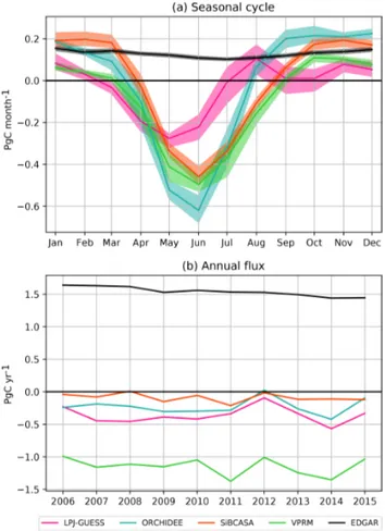
The monthly prior and posterior NEE values from the six inversions, integrated over the whole European domain (as defined in Sect. 3) and over the 10-year period of the inter-comparison, are displayed in Fig. 4. The dominant feature in Fig. 4 is the systematic differences between the seasonal cycles; i.e. each inversion shows a similar pattern in the sea-sonal cycle (large/small amplitude or timing of peak values) for each year of the simulation period.
Overall, the posterior fluxes remain within or close to the range of values defined by the different priors. In Sect. 4.2.1 and 4.2.2, we compare the prior and posterior mean fluxes and their variability, at the annual and monthly timescales. In Sect. 4.2.3 we have a first look at the sub-continental scale. Results at the grid scale are provided for completeness in the Supplement but are not further discussed in this paper.
4.2.1 Long-term mean and variability of the annual NEE budget
Prior and posterior estimates of the annual budgets of the NEE over the European domain, as well as their mean and standard deviation over the inversion period, are reported in Fig. 5.
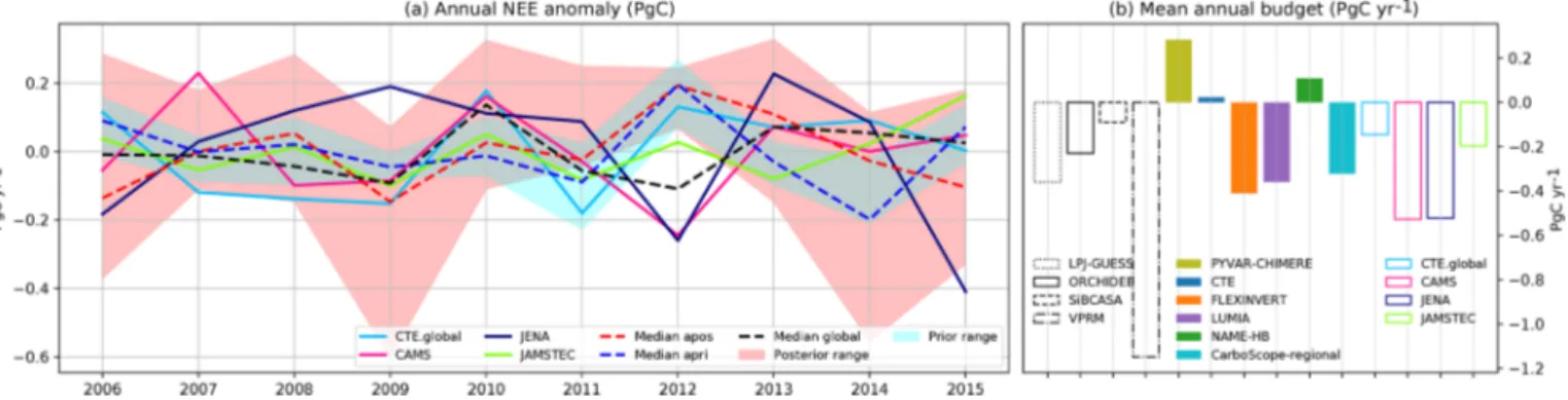
We find an ensemble mean posterior estimate of the 10-year average NEE of −0.09 Pg C yr−1(−0.16 Pg C yr−1 when excluding NAME-HB, which only covers the last 5 years), with values ranging from a net source of 0.28 Pg C yr−1 (PYVAR-CHIMERE) to a net sink of −0.41 Pg C yr−1 (FLEXINVERT). LUMIA and CarboScope-Regional estimate net sinks (−0.36 and −0.32 Pg C yr−1, respectively) and the CTE inversion yields an almost neutral NEE budget (+0.02 Pg C yr−1). Finally, besides PYVAR-CHIMERE, only the NAME-HB system finds the European ecosystems to be on average a net source of CO2to the atmosphere over our simulation period.
Over-all, the range of estimates from our inversions (0.7 Pg C yr−1) is narrower than that of the priors (1.06 Pg C yr−1between VPRM and SiBCASA).
A large fraction of the average spread is due to systematic offsets between the optimized fluxes: the standard variation of the annual flux obtained in each inversion (taken as a met-ric for the inter-annual variability, IAV) is generally much smaller than the spread of the ensemble. The standard de-viation of the annual NEE ranges from 0.11 Pg C yr−1 (LU-MIA) to 0.33 Pg C yr−1(FLEXINVERT), while the ensem-ble spread of the annual NEE is of the order of 0.8 Pg C yr−1. In the case of the CarboScope-Regional inversion, an ob-vious source for an offset from the other inversions is the prior flux from VPRM, which is much more negative than the other three priors. However, the differences between the three inversions using the NEE field from ORCHIDEE as a prior flux (PYVAR-CHIMERE, FLEXINVERT and NAME-HB) show that the biases between prior estimates can, at best, only partially explain the offsets in posterior estimates.
Figure 4. Monthly posterior fluxes, aggregated on the entire domain.
Figure 5. Annual NEE budget (positive for a source to the atmosphere and negative for a sink) for the six inversions (upper section of the array), for the four priors (middle section), and median prior and posterior fluxes (lower section). The two last columns show the mean NEE and the standard deviation of the NEE estimate, respectively, for each simulation. The colours of the cells indicate the strength and direction of the annual NEE anomaly (respective to the mean of each row; see Fig. 6 for the actual values).
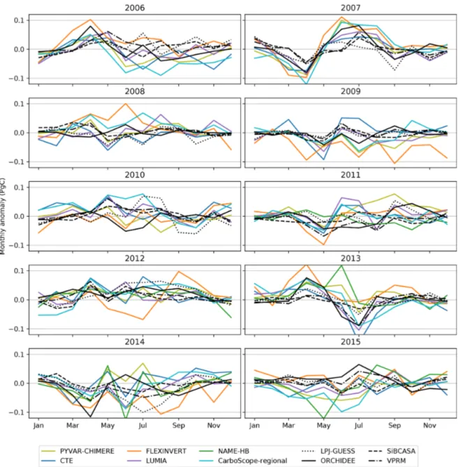
Figure 6. NEE anomalies of the six inversion posteriors and of the four priors. The median of the prior anomalies is shown as a thick blue solid line; that of the posteriors is shown as a thick red solid line. The blue shaded area shows the envelope of prior anomalies.
The annual anomalies of NEE are compared in Fig. 6, and the colours of the cells in Fig. 5 also scaled to these anomalies (with the long-term mean of each estimate taken as a reference). The ensemble spread of the posterior anoma-lies is generally much larger than that of the prior, although one system (FLEXINVERT) is contributing the most to such spread (in 2009 and 2014 for instance). The spread also strongly varies from year to year, from a minimum spread of 0.21 Pg C yr−1in 2007 to a maximum of 0.67 Pg C yr−1in 2009. In order to provide metrics less sensitive to potential model outliers, the medians of the prior (blue) and posterior (red) anomalies are shown in the Fig. 6.
There are a few consistent features, such as a clear posi-tive anomaly in 2012, already present in the priors (median of +0.19 Pg C yr−1) and further confirmed by the inversions (median value of +0.16 Pg C yr−1). In contrast to the pri-ors, however, the inversions point to a continuation of this anomaly in 2013 (+0.10 Pg C yr−1) and do not confirm the negative anomaly present in most priors in 2014. The in-versions also point to negative anomalies in 2006, 2009 and 2015 (respectively −0.16, −0.19 and −0.1 Pg C yr−1) that are clearly outside the range of prior anomalies, although the spread of the ensemble is rather large for each of these three years (> 0.5 Pg C yr−1). Overall, however, the posterior me-dian anomalies remain within or close to the range of prior anomalies for most of the 10-year period, but individual in-versions can diverge a lot from the rest of the ensemble of posterior estimates, like FLEXINVERT before 2010 and in 2014.
In summary, the inversions clearly reduce the interval of estimates regarding the mean annual NEE of the European domain (compared to the ensemble of priors) but do not ro-bustly capture the inter-annual variability of that annual flux. Analysing the differences in annual IAV is, however, com-plicated by the large spatial and temporal scales over which the fluxes are averaged: the observation network is not
homo-geneous, and the inversions may constrain some parts of the domain or times of the year better than others. In the follow-ing sections (Sect. 4.2.2 to 4.2.3) we analyse the inversion results at finer temporal and spatial scales.
4.2.2 Seasonal variability of NEE
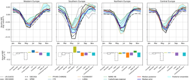
The mean monthly posterior NEE estimates for the six inver-sions together with the prior fluxes are shown in Fig. 7. At first glance, the spread of the posterior fluxes approximately matches that of the prior estimations, with very similar mean spring (May–June) uptakes, ranging from −0.24 (NAME-HB) to −0.55 Pg C per month (FLEXINVERT) in the poste-riors and from −0.28 to −0.62 Pg C per month in the pposte-riors. Winter posterior emissions are slightly higher (from +0.13 (LUMIA) to +0.32 Pg C per month in FLEXINVERT) than the priors (+0.11 to +0.23 Pg C per month). As a result, the median seasonal cycles are also very similar, with a similar phasing and a seasonal cycle amplitude of ≈ 0.55 Pg C.
This similarity between the prior and posterior ensembles hides more significant differences at the level of individual ensemble members. The phasing of the seasonal cycle is very consistent among the inversions, with terrestrial ecosystems becoming a CO2sink (flux sign switch around April and
Au-gust and with a peak uptake in June). On the contrary, the bottom-up simulations used as priors have four relatively dis-tinct seasonal patterns (see also Fig. 2).
For instance, LPJ-GUESS simulates an early peak CO2
uptake in May, which is not confirmed by the inversions (only NAME-HB yields to a similar peak). LPJ-GUESS simulates a NEE alternating between being a neutral flux and a pos-itive but small (≈ 0.1 Pg C per month) net CO2 source
be-tween July and March. This is most of the time outside or at the edge of the range of flux estimates derived from the inversions. The strong peak carbon uptake in June in OR-CHIDEE (−0.62 Pg C per month in June) clearly exceeds the lower boundary of the posterior ensemble (−0.55 Pg C