HAL Id: halshs-00459777
https://halshs.archives-ouvertes.fr/halshs-00459777
Submitted on 29 Feb 2012
HAL is a multi-disciplinary open access archive for the deposit and dissemination of sci-entific research documents, whether they are pub-lished or not. The documents may come from teaching and research institutions in France or abroad, or from public or private research centers.
L’archive ouverte pluridisciplinaire HAL, est destinée au dépôt et à la diffusion de documents scientifiques de niveau recherche, publiés ou non, émanant des établissements d’enseignement et de recherche français ou étrangers, des laboratoires publics ou privés.
evidence
Andrew E. Clark, David Masclet, Marie Claire Villeval
To cite this version:
Andrew E. Clark, David Masclet, Marie Claire Villeval. Effort and comparison income: experimental and survey evidence. Industrial and Labor Relations Review, Industrial and Labor Relations Review, 2010, 63 (3), pp.407-426. �halshs-00459777�
Volume 63
Number 3 April 2010
Article 3
2007
Effort and Comparison Income: Experimental and
Survey Evidence
Andrew E. Clark
CNRS and DELTA, Andrew.Clark@ens.fr
David Masclet
CNRS, david.masclet@univ-rennes1.fr
Marie Claire Villeval
CNRS, University of Lyon, IZA, villeval@gate.cnrs.fr
Clark, Andrew E.; Masclet, David; and Villeval, Marie Claire (2010) "Effort and Comparison
Income: Experimental and Survey Evidence," Industrial & Labor Relations Review, Vol. 63, No. 3,
article 3.
This paper considers the effect of status or relative income on work effort, combining experimental evidence from a gift-exchange game with the analysis of multi-country ISSP survey data. We find a consistent negative effect of others’ incomes on individual effort in both datasets. The individual’s rank in the income distribution is a stronger determinant of effort than is others’ average income, suggesting that comparisons are more ordinal than cardinal. In the experiment, effort is also affected by comparisons over time: those who received higher income offers or enjoyed higher income rank in the past exert lower levels of effort for a given current income and rank.
Effort, Comparison Income, Rank, Peak-End, Experiments
ANDREW E. CLARK, DAVID MASCLET, and MARIE CLAIRE VILLEVAL
The authors test the hypothesis that individual effort on the job depends both on one’s own income and on the individual’s position in the relevant income distribution. Combining experimental evidence from a gift-exchange game with multi-country ISSP survey data, they analyze the extent to which relative income affects an individual’s effort, finding that an individual’s rank in the income distribution more strongly de-termines effort than does others’ average income, which suggests that comparisons are more ordinal than cardinal. Their experiment also reveals that comparisons over time affect effort: individuals who received higher income offers or enjoyed higher income rank in the past exerted lower levels of effort for a given current income and rank.
* Andrew Clark is a research professor in economics at the Paris School of Economics, and a research fellow of the Institute for the Study of Labor (IZA) and the Center for Corporate Performance (CCP); David Masclet is a research associate professor in economics at the National Center for Scientific Research (CNRS), affili-ated with CREM (Centre de Recherche en Economie et Management) at the University of Rennes 1 and associate research fellow at CIRANO (Centre Interuniversitaire de Recherche en ANalyse des Organisations); Marie Claire Villeval is a research professor in economics at the National Center for Scientific Research (CNRS), af-filiated with the GATE (Groupe d’Analyse et de Théorie Economique) research institute at the University of Lyon 2, and a research fellow at IZA and CCP.
The authors are grateful to Charles Bellemare, David de la Croix, Fabrice Etilé, David Fairris, Lata
Gangadharan, Alan Krueger, Sabine Krüger, George Loewenstein, Andrew Oswald and the seminar par-ticipants at the AISE seminar of the Centre d’Etudes de l’Emploi; the 2005 ESA North American Meeting in Tucson, Arizona; the EALE Conference in Prague; the Utility and Inequality Conference at PSE; and the Universities of Laval, Lyon, Paris 1, and Reading for useful comments. The ISSP data were collected by independent institutions in each country, and docu-mented and made available by the ZENTRALARCHIV FUER EMPIRISCHE SOZIALFORSCHUNG, Köln. They authors are grateful to R. Zeiliger for programming the experiment presented in this paper and to the MiRe-DREES (French Ministry of Social Affairs) for a grant to support this research. Copies of the computer programs used to generate the results presented in the paper are available on request by writing to David Masclet (david. masclet@univ-rennes1.fr).
growing body of literature in econom- ics is devoted to the role of social com-parisons in explaining various phenomena, including financial market behavior, crimi-nal activity, and subjective well being. One specific area of this literature has focused on income comparisons and labor market outcomes. For example, quits are negatively correlated with a reference wage given by the average wage in the firm for similar workers; women’s labor force participation
is influenced by income comparisons; and rank in the local income distribution is a good predictor of migration. These behaviors mostly concern job choice. Little is known, however, about the impact of relative income on how hard employees actually work on the job, even though efficiency wage theories are built on the concept of income comparisons, and relative concerns are appealed to as an explanation of wage compression (Frank 1984).
407
A
Industrial and Labor Relations Review, Vol. 63, No. 3 (April 2010). © by Cornell University.
In this paper we attempt to fill this gap by analyzing the influence of income compari-sons on effort using both experimental and survey data. We suggest that such income comparisons may explain why some of the empirical evidence on the wage–effort rela-tionship is mixed. Though it is commonplace to assume that wages have incentive effects, or that higher wages make up for higher effort in a compensating differential set-up, higher wages are not always associated with greater effort in empirical work. This has variously been explained by a crowding-out effect of monetary rewards on intrinsic mo-tivation (Frey and Oberholzer-Gee 1997), supra-optimal motivation generating choking under pressure (Ariely et al. 2009), or an earnings target that bounds effort at some threshold (Camerer et al. 1997). Here we test an alternative hypothesis—that individual effort depends on both one’s own income and the individual’s position in the relevant income distribution. In light of their com-parisons with others, those who are paid relatively well work harder. We test whether others’ incomes matter, and ask, given one’s own income, which of relative income and income rank in the reference group is most important in determining effort. That is, are social comparisons cardinal or ordinal? We further ask whether income comparisons are not only horizontal (that is, comparable to other individuals at the same point in time) but also intertemporal, so that the time profile of individual income or rank helps to explain current effort at work.
Conclusive empirical proof of the exis-tence of social comparisons is elusive since it is difficult to know to whom individuals compare themselves, and because indi-viduals’ behavior may be correlated within a group—not because they compare to each other, but because they are exposed to com-mon unobserved environmental factors, or because they share similar characteristics. The experimental approach adopted here has the double advantage of defining a
priori the reference group and limiting any
contextual effects. In addition, our approach relies on actual and costly decisions rather than on subjectively reported behavior. Un-like experimental data, survey data offer the
advantage of larger sample sizes and mitigate the criticism that laboratory experiments are to an extent unrealistic. The combined use of both survey and experimental data is still relatively recent (Fehr et al. 2003; Carpenter and Seki 2010; Brown et al. 2008) and can be interpreted as a joint test of robustness. If consistent patterns emerge in both types of data, we can be more confident in the ex-ternal validity of our laboratory experiments. Our experiment extends the standard gift-exchange game between an employer and an employee by introducing income compari-sons between employees from different firms. The reference group for employees consists of employees in other firms participating in the same experimental session. In this between-firm comparison design, employees are pre-sumed to be similar and are thus expected to receive the same equilibrium wage. In the first stage of this game, the employer offers a wage contract and in the second, employees who accept the contract decide on their effort level. In one treatment we can identify income comparisons as we inform employees, before they choose their effort level, about the wages offered by a sub-set of other employers in the labor market. Testing the robustness of our experimental results required a dataset with information on discretionary effort that closely resembled the experimental design. The survey data come from the 1997 wave of the ISSP (International Social Survey Program), which includes information on both earnings and self-reported discretionary effort. The questions asked in this survey are extraordinarily close to the context of the gift-exchange game, in that the employee’s reported effort is explicitly oriented towards improving the firm’s outcome.
Literature
The existing literature on social com-parisons can be broadly divided up into two strands: that on behavior and that on utility. This division can be illustrated by a direct utility function:
(1) Ui = U(ai, aj, …) for j ≠1
in which individual i’s utility,Ui , depends on both her own actions and those of relevant
others, ai and aj. This utility function most
often gives rise to a decision rule for i’s utility-maximizing behavior a*
i as:
(2) a*
i = f(aj, …).
The behavior and utility approaches to social interactions attempt to find empirical coun-terparts to (2) and (1) respectively. There are a number of drawbacks to the behavioral approach, the first of which is that data on behavior are not always particularly accurate. Second, behavior often reflects the intersec-tion of supply and demand, whereas we are interested here in individuals’ preferences. Third, under separability conditions,1 others’
behavior can affect one’s own utility, but not one’s behavior. There are equally problems with the utility approach, via equation (1). In particular, we do not necessarily know how to best measure individual utility, Ui.
Interactions in behavior have been widely modeled econometrically, despite the iden-tification problems emphasized by Manski (1993).2 Many of these studies have concluded
that social interactions do indeed influence behavior, in the sense that “if you do more of something, then I am likely to do more of it as well.” One interpretation of this maxim is that this correlation reflects a concern for status or relative standing. Another is that this correlation reflects the process by which individuals may be learning from each other about how pleasant or dangerous goods or activities are (so that their behaviors are cor-related), rather than caring about their status. Rival explanations emphasize the potentially key role of common omitted variables such as contextual effects; however, much of what is published in the empirical literature is very careful to try to account for these.
An alternative approach to identifying in-teractions appeals to proxy measures of utility, such as life satisfaction, job satisfaction, and
happiness (Ferrer-i-Carbonell, 2005; Clark, Frijters, and Shields 2008). Perhaps because of a scarcity of surveys that measure both proxy utility and behavior adequately, most attention has been concentrated on the role of income comparisons in the utility func-tion. Empirical estimation has thus mostly been based on the indirect utility function,
Vi, testing specifications such as
(3) Vi = V(yi, yj, …) for j ≠ i
in which utility depends on one’s own and relevant others’ incomes, yi and yj respectively, rather than its direct counterpart (1) above.
Both the behavior and utility approaches require that the reference group be identi-fied—to whom does the individual compare? There are a number of potential candidates, including the individual’s peer group (those who share the same characteristics), others in the same household, spouse/partner, friends, neighbors, work colleagues, and the individual him- or herself in the past. An approach to modeling social comparisons which combines both of the above would be to consider i’s behavior, ai as a function of both his or her own income and that of his or her reference group, yi and yj:
(4) ai = a(yi, yj, …).
This can be operationalized empirically as (5) ai = A0 + byi + fyj + g'Xi + ei.
The b coefficient in equation (5) shows the extent to which individual behavior, ai , de-pends on the individual’s own income. If only one’s own income matters in explaining i’s behavior, then the estimate of f will be insig-nificant. Alternatively, if income comparisons matter for behavior then both b and f will be significant. If action a is normal then we expect b > 0 and f < 0. This is the empirical approach that we take in this paper.
The behavior we consider here is effort expended at work. We ask whether workers’ effort, ei , depends on how much others earn, modeling
(6) ei =e(yi , y*, …)
where we expect e1 > 0 but e2 < 0. Here y* is
some transformation of the income vector
1Formally, d
2U
i
daidaj
= 0.
2 Recent contributions in this vein have analyzed
sav-ing (Duflo and Saez 2002), tax evasion (Fortin, Lacroix, and Villeval 2007), labor supply (Aronsson, Blomquist, and Sacklén 1999), and students’ success at school (Arcidiacono and Nicholson 2005; Sacerdote 2001).
of other people who are in individual i’s reference group. The idea is that individual
i has a comparison or reference person or
group j and reduces his or her own input or effort as reference income rises, given his or her own wage.
Much of the efficiency wage literature is based on this idea of the comparison of one’s own wage to those of co-workers (Akerlof and Yellen 1990) or to that of workers in other firms (Summers 1988; Johansen and Strøm 2001).3 However, to the extent of our
knowledge, empirical evidence that workers’ current effort does in fact depend on rela-tive income or on one’s own past income remains slight.4
A recent literature in experimental economics has sought evidence of social comparisons among co-workers. In the first stage of the game proposed by Charness and Kuhn (2007), a principal can offer different wages to his or her two employees. These employees may possess either homogeneous or heterogeneous ability levels, but they know neither the direction nor the magnitude of these differences. In the second stage of the game, employees choose their level of effort, and according to the treatment, wages are either public or private. Income comparisons are shown to affect employees’ behavior only weakly whereas firms reduce income differentials between co-workers for fear of low-effort retaliation from the lower-paid employee. In other words, firms anticipate a negative effect from income comparisons on
effort that is not actually observed in workers’ behaviors. This wage compression effect was also found by Güth et al. (2001) in a game in which information about the contracts offered to each employee was manipulated. They demonstrated that principals tend to re-duce the income differential between agents when contract information is made public.
In these experiments, productivity differ-ences are introduced between co-workers in order to motivate firms to vary their wage offers. The weak reaction by employees to subsequent income comparisons may show that workers consider productivity differences to be a fair source of income differentials. In our experiment, however, all employees ex-hibit the same productivity, each firm employs only one worker, and income differences result from firms’ various choices (and not from any skill differences between workers). Gächter and Thoeni (2009) provided another experimental test using the strategy method. Subjects were asked to report their effort decision in reaction to various hypothetical income distributions. They identified a large subset of individuals who reduced their effort when faced with income inequality. In our experiment, incomes are actually chosen by real firm-subjects, and we infer the influence of income comparisons from individuals’ observed effort decisions.
Empirical Strategy
Our empirical strategy is based on the joint use of experimental data produced in the laboratory and on survey data. The survey data analysis helps to check the external valid-ity of the experimental evidence. When we evoke income comparisons here, we define income as the wage offered by the employer to the employee; that is, we do not take into account the cost of effort that will depend on the level of effort chosen by the employee.
Experimental Design
The game. We identify the impact of
in-come comparisons on effort using a version of the standard gift-exchange game (Fehr, Kirchsteiger, and Riedl 1993). Each session involves twenty subjects who are divided into two groups, ten in the role of firms and ten in
3Wage comparisons and effort have also been evoked
in the business-cycle literature (Collard and de la Croix 2000).
4One fascinating exception is Mas (2006), who
exploited a natural experiment to consider the rela-tionship between relative wages and effort. New Jersey police unions bargain over wages with their municipal employer, with disputes being settled by an outside arbitrator. Controlling for the actual pay level awarded, Mas found that 12% more crimes per capita are solved (cleared) when unions win their case compared to when they lose. This is interpreted as evidence that police ef-fort depends on pay relative to some reference point. By way of contrast, most of the experimental work on the impact of others’ income tests for inequality aversion and focuses on distribution decisions through choices over tax rates, transfers, or the distribution of income (see Cowell 2004).
the role of employees. Roles are attributed at random and are kept constant throughout the session. All employees have the same charac-teristics, in contrast to Güth et al. (2001) and Charness and Kuhn (2007). Workers do not differ in ability and thus do not have to form beliefs about the relationship between other employees’ productivity and their incomes. A Benchmark Treatment and an Information Treatment were implemented.
The Benchmark Treatment consists of the standard gift-exchange game. The use of this standard game ensures that our results can be directly compared to those from previous experiments before we introduce a new ele-ment in the Information Treatele-ment. In every period of the game, each firm is matched randomly with an employee. There are ten periods and each period consists of two stages. In the first stage, the firm offers a con-tract consisting of a wage w ∈ [20, 120] to its employee. In the second stage, the em-ployee decides whether to accept or reject the contract. If the contract is rejected, both the firm and the employee receive nothing. Upon acceptance, the employee must choose his or her level of effort, e ∈ [0.1, 1].5 The
greater the employee’s effort, the higher the firm’s profits; at the same time, the greater
the effort cost c(e) borne by the employee. This effort cost is convex, as shown in Table 1.
In the standard gift-exchange game, the employer’s payoff is
pp = (n – w)e
where n is an exogenous redemption value; in our experiment, n = 120. This expression guarantees that the firm does not incur a loss even if the employee chooses the minimum level of effort. The employee’s payoff is pA = w – c (e) – 20
with a fixed labor market participation cost of 20 (corresponding to travel costs, say).6
These payoff functions are common knowl-edge for all participants. At the end of the period, the firm is informed about the level of effort chosen by the employee, and both the firm and the employee are informed about their respective payoffs. In each new period, the pairs of firms and employees are randomly reshuffled. We implement a perfect stranger matching protocol in the sense that no agent is matched with any principal more than once, which, again, is common knowledge in that it is printed in the instructions. This allows us to rule out any reputation-building behavior (Gächter and Falk 2002).
The Information Treatment is similar in structure except that at the end of the first stage, after the firm’s income offer is revealed, the employee is told about the income offers that four other employees received from their firms in the same period. Employees can thus compare their own income to the income offered to other, ostensibly similar, employees on the labor market (but not co-workers) before rejecting or accepting the
5It is important to separate these two stages in order
to respect the standard gift-exchange game and to check the comparability of our results in the Benchmark Treatment to those in previous work. As others have argued in the literature on gift-exchange games, this design allows us to disentangle the effort decision from the job entry decision and to analyze whether income comparisons exert the same influence, if any, on both decisions. Combining the decision to accept an offer and the choice of effort in one single stage would simplify the design, but this requires that the decision to accept a contract offer and effort choice be determined in the same way, or that rejecting a contract is equivalent to completely shirking one’s responsibilities on the job. As the results will show, we reject this hypothesis. In any case, there is no guarantee that an agent would choose to exert zero effort were he or she not allowed to reject a contract offer.
6This fixed cost, which must be covered by firm’s
wage offer, exists only to avoid having a minimum wage of zero in the set of firm’s actions; it has no implications for the theoretical predictions of the game.
Table 1. The Cost of Effort in the Experiment
Effort e 0.1 0.2 0.3 0.4 0.5 0.6 0.7 0.8 0.9 1
contract, and thus before choosing effort. We choose to display only partial information about other income offers (in each period, four other randomly-chosen income offers, instead of the whole distribution) to produce a greater variety of income distributions within the reference group. In addition, this procedure allows the relative income effect to be identified separately from any period effect. In contrast to the employee, the firm is not informed about the other firms’ income policies, reducing the likelihood that firms will behave differently in the two treatments. This decision is justified by the fact that we are mainly interested in the comparison between employees.
Equilibrium of the game. The equilibrium of
this game with selfish and rational players is a minimum wage–minimum effort pair of decisions, [w = 20, e = 0.1]. The minimum wage contract should be accepted since the employee has no better alternative. Equally, the employee should accept the contract and choose the same (minimum) effort level in both treatments since the incomes offered by other firms do not enter into the standard individual utility function. Firms should thus offer the same (minimum) income in both treatments. It is possible, however, that in both treatments, income and effort will rise above their theoretically predicted levels. Existing research has demonstrated that employees typically reciprocate high income offers by choosing high effort levels that increase the firm’s payoff; conversely, they reciprocate low income offers by choosing low effort levels that decrease the firm’s payoff (Fehr, Gächter, and Kirchsteiger 1997).7
In addition, information about the income distribution may affect effort in the Informa-tion Treatment if individuals are sufficiently sensitive to income comparisons. If subjects make horizontal comparisons (that is,
com-pare themselves to other employees), we may expect effort to be positively correlated with both relative income and income rank. And yet, since firms in this game are never informed about the income distribution, there is no reason why their behavior should differ across treatments.8
Procedures. The experiment was conducted
in the experimental laboratory at GATE, Lyon, France, using the Regate software (Zeiliger 2000). A total of 120 undergraduate students from three local Engineering and Business schools participated in one of the six sessions organized. Two of these concerned the Benchmark Treatment and four the In-formation Treatment. No one participated in more than one session. Upon arrival, the subjects drew a label from an envelope, indicating the name of their computer. The instructions (see the Appendix) were dis-tributed and read aloud. The subjects then filled out a questionnaire that allowed us to check their understanding of the rules of the game. Questions were answered in private.
The program paired firms and employees randomly and anonymously, and the subjects subsequently discovered their role (firm or employee). Since the game was repeated 10 times under a perfect stranger matching protocol, each firm made an income offer to each of the employees. This yielded a total of 200 wage offers in the Benchmark Treat-ment and 400 wage offers in the Information Treatment. Each employee made 10 contract-acceptance decisions and, if the contract was accepted, chose an effort level. In the next section we analyze these effort decisions.
Each session lasted one hour on average, including the payment that was carried out in a separate room. The experiment was conducted in experimental currency units with 100 points equal to 4 Euros. Each subject earned on average €14 from the experiment, including a show-up fee of €4. This indicates that in each period, the subjects earned on average €1.
Compared with survey data, this experi-mental approach presents many
advantag-7One might argue that individuals may also
recipro-cate higher income rank and higher relative income with higher effort in the Information Treatment. However, in our experiment, firms were never informed about the income distribution. As a consequence, ranking cannot be considered as intentional on the part of the employer. In any case, employees would presumably only reciprocate relative income if it were valuable to them, which is exactly what we want to demonstrate.
8A firm cannot know whether a lack of reciprocity
es—income is perfectly measured, effort is observed directly instead of being self-report-ed, and the reference group is controlled. However, the artificiality of the laboratory may cast doubts on the external validity of the experimental results. For these reasons, we complement our experimental analysis with survey evidence on income and effort.
Survey Data on Work Effort
The survey data, multi-country and cross-section, come from the 1997 Work Orienta-tions module of the International Social Survey Programme, the ISSP (the data and documentation are freely available from http://www.issp.org). The key variables in our empirical analysis are effort, earnings, and hours of work. Income is measured as individual yearly labor market earnings, converted to U.S. dollars using Purchasing Power Parities from the Organization for Economic Cooperation and Development (OECD). Hours of work are measured at the weekly level.
The variable we wish to explain is effort at work, which is almost never observed directly in survey data. To compare our experimental evidence to (larger-scale) survey data, we require a survey in which employees report their willingness to exert effort in order to improve their employer’s outcome, as in the experimental set-up where the employee provides extra effort at his or her own cost in order to increase the employer’s earnings. The question we appeal to in the ISSP data is crafted to measure discretionary effort and is thus arguably well suited to our analysis. All those employed are asked to indicate the extent to which they agree with a number of statements. One of these is, “I am willing to work harder than I have to in order to help the firm or organization I work for to suc-ceed.”9 This question is remarkably close to
the context of the gift exchange game, in
which any level of effort above the minimum is voluntary and increases the firm’s profit but decreases the employee’s payoff. It is reasonable to assume that “helping the firm to succeed” in the survey data is analogous to improving its payoff, and conversely that increasing the firm’s earnings in the experi-ment is comparable to helping it to succeed. The weighted distribution of the five pos-sible responses to this question in the 1997 ISSP is shown below in percentages.
Strongly agree 16.7%
Agree 42.4%
Neither agree nor disagree 24.2% Disagree 12.0% Strongly disagree 4.5%
Keeping only full- or part-time employees aged 16–65 yields a sample of 12,000 observa-tions over 17 countries (considering the two Germanies separately). Missing values on earnings, hours of work, and effort finally produce a regression sample of around 10,000 observations.
We are interested in describing differ-ences in the response to the effort question between individuals, and we first examine the cross-country pattern in discretionary effort. To do so, we allocate a value of 5 to “strongly agree” through to a value of 1 for “strongly disagree” to the question described above. Table 2 illustrates the number of observations and mean effort, ranked by country from the lowest to the highest aver-age effort. The countries in our study vary in the degree of social reciprocity that workers exhibited. Workers in Mediterranean coun-tries are ranked broadly towards the bottom whereas workers in Anglo-Saxon countries are on average more willing to work hard to help their firm or organization. Portugal is an exception to this general rule, appearing toward the top of the ranking.10
9This is similar to variables used in management
to capture organizational commitment (see Jaworski and Kohli (1993)). It could also, of course, reflect the employee’s effort to prevent the firm going bankrupt; however, even in this context, employees provide costly effort in order to improve the firm’s outcome.
10There is a strong correlation between
unemploy-ment and the mean of this effort variable. The average OECD standardized unemployment rate in 1997 of the lowest seven countries in the ranking was 12.3%, opposed to 5.9% for the ten highest-ranked. Both the Pearson and Spearman correlations between mean effort and the unemployment rate are significant at higher than the 2% level. One interpretation is that social reciproc-ity allows firms and employees to attain Pareto-superior employment outcomes.
The main thrust of our paper is, con-ditional on country, to see how workers’ discretionary effort is related to individual demographic and job characteristics. We are especially interested in the role of income on work effort. We control not only for individual income and hours of work but also for refer-ence group income. This latter is defined in a similar way to that in the Leyden school—by calculating average values of income over fairly broad demographic groups11 —in this
case country, gender, education, and age. There are three education groups (up to 10 years of education, 11 to 13 years of educa-tion, and more than 13 years of education), and three age groups (16–29, 30–44, and 45–65). There are thus 17 (country) * 2 (sex) * 3 (education) * 3 (age) = 306 reference groups. These average income measures are called comparison income in the regression tables and correspond to y* in equation (6)
above.12 Comparison income for individual i
in cell j is calculated excluding i’s own income.
Results
Effort may be influenced by own income, by relative income or income rank, or by the income the individual received in the past if there are intertemporal comparisons. We estimate discretionary effort equations on both experimental and survey data to de-termine whether income comparisons affect individual effort behavior.
Effort and Comparisons to Others
The average wage offered by firms in the experiment was 53.51 (s.d 19.7) in the Benchmark Treatment and 53.09 (s.d. 20.0) in the Information Treatment (where wage offers were constrained to lie between 20 and 120). Both average figures are clearly above the equilibrium wage of 20 (one-tailed
t-test, p<.0001) but are not significantly dif-ferent from each other. Firms do anticipate reciprocity from their employees, but they do not change their wage offers when income comparisons appear.
Two different specifications of comparison income are used, the first being normalized rank, defined as rank in cell or group/num-ber of observations in cell or group, with a correction for ties. This is a measure of how the individual’s income is ranked rela-tive to the other members of the reference group in the Information Treatment and in the ISSP survey data (and not relative to all individuals). In the experimental data, the rank determines the position of the subject relative to the four other group members for whom wage information was revealed. This measure is bounded between just over zero for the bottom-ranked income in the cell to one for the top-ranked income. The second comparison measure is average reference group income, excluding the individual’s own income. Average and individual earn-ings levels are expressed in experimental
Table 2. Mean Discretionary
Effort by Country: ISSP 1997
Employees Mean Country interviewed Effort
No. % USA 775 6.47 3.93 Canada 546 4.55 3.75 Portugal 843 7.03 3.71 Switzerland 1,727 14.41 3.65 Denmark 600 5.01 3.64 Great Britain 545 4.55 3.63 Japan 607 5.06 3.62 Hungary 626 5.22 3.60 Czech Republic 526 4.39 3.60 Norway 1,366 11.40 3.59 East Germany 261 2.18 3.59 West Germany 648 5.41 3.52 Sweden 793 6.62 3.42 Spain 387 3.23 3.35 Poland 564 4.71 3.26 Italy 475 3.96 2.96 France 698 5.82 2.85 Total 11,987 100.00 3.55
Note: The question is “I am willing to work harder than I have to in order to help the firm or organization I work for to succeed?” with responses coded from 5 for “strongly agree”
through to 1 for “strongly disagree.”
11See for example van de Stadt, Kapteyn, and van
de Geer (1985).
12This cell-average approach does not suffer from the
identification problems that occur when y* is predicted
in a regression framework since the cell-average income is not a linear function of the X variables (the variables that define the cells—country, age, gender and education).
currency units in the experimental data, and in thousands of U.S. dollars per month in the ISSP data.
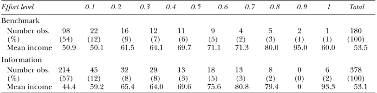
We estimate the influence of income com-parisons on effort in the experimental data via random effects tobits. The use of tobit models is justified by the number of left-censored observations in the sample. Table 3 displays the distribution of effort levels and mean income per effort level, illustrating that minimum effort (0.1) was chosen 98 times out of 180 in accepted contracts (54.4%) in the Benchmark Treatment, and 214 times out of 378 in accepted contracts (56.6%) in the Information Treatment.13 Not taking this
data censoring into account would likely bias the coefficients.
Table 3 indicates a positive relationship between income and effort in both experi-mental treatments, which is typically observed in the gift-exchange game (Fehr, Gächter, and Kirchsteiger 1997) and is consistent with social motivations leading to reciproc-ity. Though the income–effort relationship looks somewhat steeper in the Information Treatment, the joint presence of income and comparison income makes such bivariate
conclusions untrustworthy. The main effort regression results using the experimental data are shown in Table 4, and those based on the ISSP survey data are illustrated in Table 5. Table 4 consists of two panels. The left panel displays the results of six regres-sions in which the dependent variable is the effort choice of subjects who accepted a contract offer. The right panel, which we will discuss below, presents the results of alternative specifications that check the ro-bustness of the results. Most regressions are estimated as tobits, which account for both left- and right-censoring (the first of which is endemic in our data). In addition, since each subject is observed a number of times (up to 10 times if the subject accepts all the contract offers), we appeal to panel data methods and estimate all of the regressions in the left-hand panel with random effects. In the Benchmark (Information) Treatment, 20 (22) contracts were rejected. Our left-hand panel sample thus consists of 180 effort deci-sions in the Benchmark Treatment and 378 in the Information Treatment.
Regressions (1) and (3) consider the role of one’s own income in the Benchmark and Information Treatments, respectively. Regres-sions (2) and (4) add normalized income rank as an explanatory variable: Higher values of this rank variable correspond to higher positions in the reference group income distribution. Since subjects are not informed about their income rank in the Benchmark Treatment, this “placebo” variable should be insignificant there, unless income and rank are strongly collinear. The last two re-gressions in the left-hand panel refer to the Information Treatment only. Regression (5)
Table 3. Average Income and Effort Levels in Accepted Contracts
Effort level 0.1 0.2 0.3 0.4 0.5 0.6 0.7 0.8 0.9 1 Total
Benchmark Number obs. 98 22 16 12 11 9 4 5 2 1 180 (%) (54) (12) (9) (7) (6) (5) (2) (3) (1) (1) (100) Mean income 50.9 50.1 61.5 64.1 69.7 71.1 71.3 80.0 95.0 60.0 53.5 Information Number obs. 214 45 32 29 13 18 13 8 0 6 378 (%) (57) (12) (8) (8) (3) (5) (3) (2) (0) (2) (100) Mean income 44.4 59.2 65.4 64.0 69.6 75.6 80.8 79.4 0 93.3 53.1
13If we consider individuals instead of decisions, we
observe that only a minority of subjects behave self-ishly. Defining as selfish individuals those subjects who choose the minimum effort in at least 8 periods out of 10, 35% of the people in the Benchmark and 27.5% in the Information Treatment are considered selfish. We cannot, however, determine whether this difference is inherent in the nature of the subjects involved in the two treatments or if it is attributable to the dissemination of income information. If it is the latter, some fraction of minimum effort decisions are motivated by social comparisons rather than by selfishness.
replaces income rank by average reference group earnings (excluding own income), and regression (6) includes both income rank and average group earnings. All of the ex-perimental effort regressions control for both gender and number of post-baccalaureate years of education.
Table 5 reports the results of four analo-gous estimations on the ISSP survey data, in which the dependent variable represents the degree of willingness of workers to work harder to help the company or organiza-tion to succeed. Each individual is observed only once and we have 9,854 observations. Ordered probit regressions are estimated since the survey effort question allows five ordered responses. We follow the same logic as for the experimental data—regression (1) includes one’s own income only; regression (2) adds normalized income rank; regression (3) replaces rank by comparison income; and regression (4) estimates the joint influence of own income, rank and average reference group income. We also control for hours of work, age, gender, education and marital status, and we include country dummies. The standard errors in this Table are clustered at the reference group level.14
The results in Tables 4 and 5 show that effort is strongly correlated with one’s own absolute income at the 1% level in both treatments of the experimental data and in the survey data. Regressions (4) and (2) in Tables 4 and 5, respectively, illustrate the influence of others’ income. That is, nor-malized income rank attracts a positive and significant coefficient conditional on one’s own income. For the same number of dol-lars/experimental units earned, individuals are willing to work harder the higher their position is in the reference group income distribution. Unsurprisingly, normalized in-come rank is insignificant in the Benchmark Treatment (see regression (2) in Table 4), where individuals are unaware of their rank. In the experiment (column 4), a rise in rank of one position (out of five) increases effort
by 0.57 (= 0.20*2.87), which is equivalent to a wage increase of 6.52 for given rank. Com-pared to average income per period (53.09), this latter represents a wage rise of 12.3%. The rank/income elasticity is thus 0.614 (= 12.29/20). In the survey data, a 20% rank increase has the same effect on effort as an extra $623 per month, which is 33% of aver-age income, yielding a rank/income elasticity of 1.6. This higher elasticity may reflect the wider distribution of income in the survey data, the fact that rank matters more “in real life,” or that rank is more important when reputation-building is possible.
The experimental evidence thus points to income position within the reference group as being an important determinant of how much discretionary effort workers provide, over and above the actual income they receive, the latter of which has been the focus of the literature to date. This is confirmed by the survey data analysis.15 This, to our knowledge,
is one of only a small number of empirical findings pointing to relative income and sta-tus as a determinant of employees’ behavior. In regressions (5) and (3) in Tables 4 and 5, respectively, average income in the reference group attracts a negative coefficient, which is significant only for the experimental data. If we include both normalized rank and refer-ence earnings in the same regression (col-umn 6 in Table 4 and col(col-umn 4 in Table 5), this marginally significant effect disappears, whereas the coefficients associated with rank remain positive and significant. Our second key result is therefore that ordinal compari-sons, as measured by normalized rank in the income distribution, are more powerful predictors of employee behavior than are cardinal comparisons, that is, from others’ earnings expressed in currency units.16
14Income is entered in levels. Entering all of the
cardi-nal income variables as logs produces similar results but is not preferred by the data (the log likelihood is lower).
15The ISSP results are largely unchanged when we
drop the 20% of observations that are found in reference groups with 30 observations or less, or if we use a less ag-gregated reference group by dropping education or age.
16This result concurs with that in Brown et al. (2008),
where income rank is shown to outperform average reference group income in three satisfaction equations (influence over the job, achievement, and supervisor’s respect). For the fourth dependent variable, satisfaction with pay, both rank and reference group income attract significant coefficients.
Ta bl e 4. E ff or t, R an k an d C om pa ri so n I n co m e in th e E xp er im en ta l D at a R eg re ss io n m od el s R ob us tn es s te st s T re at m en ts B en ch m ar k T re at m en t In fo rm at io n T re at m en t I nf or m at io n tr ea tm en t Ef fo rt in Ef fo rt fo r Ef fo rt in D ep en de nt V ar ia bl es Ef fo rt in a cc ep te d co nt ra ct s ac ce pt ed c on tr ac ts al l o ff er s A cc ep ta nc e ac ce pt ed c on tr ac ts R E G L S R E R E R E R E R E R E To bi t w ith R E R E R E w ith c lu st er ed R E M od el s To bi t a To bi t To bi t To bi t To bi t To bi t cl us te re d S. E. To bi t G L S b Pr ob it S. E. To bi t (1 ) (2 ) (3 ) (4 ) (5 ) (6 ) (7 ) (8 ) (9 ) ( 10 ) (1 1) (1 2) (1 3) O w n I n co m e 0. 10 6* ** 0. 08 5* ** 0. 12 1* ** 0. 08 8* ** 0. 11 7* ** 0. 09 1* ** 0. 09 3* ** 0. 11 2* ** 0. 04 9* ** 0. 04 6* ** 0. 14 4* ** 0. 04 5* ** 0. 08 8* ** (0 .0 17 ) c (0 .0 26 ) (0 .0 11 ) (0 .0 15 ) (0 .0 11 ) (0 .0 16 ) (0 .0 18 ) (0 .0 20 ) (0 .0 08 ) (0 .0 08 ) (0 .0 44 ) (0 .0 10 ) (0 .0 15 ) In co m e R an k 1. 34 9 2. 87 1* ** 2. 40 1* * 2. 79 2* * 2. 23 5* 1. 19 3* * 1. 02 9* * 0. 99 7 1. 23 5* 2. 88 6* ** (1 .3 96 ) (1 .0 38 ) (1 .1 43 ) (1 .2 60 ) (1 .3 59 ) (. 05 37 ) (0 .5 19 ) (1 .2 60 ) (0 .7 17 ) (1 .0 47 ) C om pa ri so n I n co m e –0 .0 34 ** –0 .0 19 0. 02 6 (0 .0 17 ) (0 .0 19 ) (0 .0 29 ) M al e –3 .2 31 * –3 .8 75 * –1 .2 48 –1 .1 61 –1 .3 89 –1 .2 43 –0 .7 74 –0 .7 29 0. 03 4 0. 00 1 –0 .2 05 –1 .1 58 (1 .9 63 ) (2 .0 14 ) (1 .3 77 ) (1 .3 62 ) (1 .3 74 ) (1 .3 65 ) (1 .6 31 ) (1 .7 10 ) (0 .5 40 ) (0 .5 37 ) (0 .6 66 ) (1 .3 60 ) M al e* In co m e 0. 03 13 0. 02 4 0. 01 5 0. 03 9 0. 01 6 0. 04 2 0. 04 8 0. 07 5 0. 01 9 0. 01 9 0. 01 9 0. 03 9 (0 .0 24 ) (0 .0 35 ) (0 .0 17 ) (0 .0 29 ) (0 .0 16 ) (0 .0 29 ) (0 .0 46 ) (0 .0 48 ) (0 .0 14 ) (0 .0 13 ) (0 .0 20 ) (0 .0 29 ) M al e* R an k 1. 46 9 –2 .2 09 –2 .3 82 –3 .0 19 –5 .0 16 –1 .1 18 –1 .1 05 –0 .9 52 –2 .2 09 (2 .3 26 ) (1 .9 77 ) (1 .9 86 ) (2 .8 42 ) (2 .8 54 ) (0 .9 43 ) (0 .9 14 ) (1 .0 06 ) (1 .9 75 ) Ye ar s of E du ca ti on 1. 28 4 1. 27 7 0. 04 4 0. 04 5 0. 07 1 0. 06 1 –0 .1 73 –0 .1 06 –0 .1 68 –0 .1 62 –0 .1 53 0. 04 6 (0 .8 50 ) (0 .8 51 ) (0 .4 03 ) (0 .4 01 ) (0 .4 00 ) (0 .4 00 ) (0 .3 58 ) (0 .3 28 ) (. 01 70 ) (0 .1 81 ) (0 .1 99 ) (0 .4 01 ) In ve rs e M ill s R at io 0. 12 8 0. 17 7 (0 .5 71 ) (1 .5 78 ) C on st an t –1 1. 12 8* ** –1 1. 09 9* ** – 5. 91 8* ** – 6. 06 6* ** – 4. 06 2* –5 .0 29 ** –5 .4 65 ** * –7 .5 39 ** –0 .4 40 –0 .2 17 –4 .2 24 ** * –0 .4 89 –6 .0 95 ** * (3 .6 87 ) (3 .6 84 ) (1 .9 34 ) (1 .9 29 ) (2 .1 06 ) (2 .1 93 ) (2 .3 45 ) (2 .8 07 ) (0 .8 13 ) (0 .8 54 ) ( 1. 35 0) (1 .0 19 ) (1 .9 45 ) N um be r of o bs . 18 0 18 0 37 8 37 8 37 8 37 8 37 8 37 8 40 0 40 0 40 0 37 8 37 8 L ef t-c en s ob s. 99 99 21 4 21 4 21 4 21 4 21 4 21 4 22 21 4 21 4 R ig h t-c en s ob s. 1 1 6 6 6 6 6 6 6 6 6 R 2 0. 50 7 0. 49 L og -li ke lih oo d –2 15 .6 92 –2 14 .1 51 –4 27 .3 39 –4 23 .4 48 –4 25 .2 64 –4 22 .9 78 –4 67 .0 98 –4 82 .7 57 –6 89 .2 31 –4 8. 00 2 –4 23 .4 42 W al d χ 2 10 8. 31 11 0. 44 22 6. 48 23 6. 08 23 0. 63 23 6. 58 36 2. 66 34 2. 15 14 .4 6 17 3. 71 23 6. 73 a R E T ob it =r an do m e ff ec ts to bi t b R E G L S= ra n do m e ff ec ts g en er al iz ed le as t s qu ar es cSt an da rd e rr or s in p ar en th es es ** * Si gn ifi ca n t a t t h e 0. 01 le ve l; ** a t t h e 0. 05 le ve l; * at th e 0. 1 le ve l. A ll of th e re gr es si on s i n th is ta bl e in cl ud e pe ri od d um m ie s; a ll of th e re gr es si on s e xc ep t ( 11 ) in cl ud e se ss io n d um m ie s.
Other results in Table 4 show that in the experimental data, gender and education have a marginally significant negative effect on effort in the Benchmark Treatment but have no significant impact in the Information Treatment. In the ISSP data, controlling for rank or average income, effort is higher for men, the married and the higher-educated. The difference between the experimental and the ISSP data may reflect the far smaller variance in the demographic variables in the student subject-pool than in the ISSP data. Last, the estimates on the country dummies in the ISSP regressions (not shown) largely reproduce the effort ranking in Table 2. Robustness Checks To check the robustness of our experimen-tal results, we have considered a number of alternative specifications, some of which are reported in the right-hand panel of Table 4. For the sake of simplicity, we only report the estimations that include both own wage and normalized rank. First, columns 7 and 8 reproduce columns 4 and 6 yet allow for a less restrictive form of correlation between error terms at the individual level than ran-dom effects. The estimation method here is a tobit with clustered standard errors at the individual level. Similar estimations with clustered standard errors have been carried out for each of the previous models. The primary significance of these regressions is that the results in the left-hand panel of Table 4 are unaffected by this clustering. Cluster-ing increases the standard errors, but both own income and rank remain significant in columns 7 and 8.
The main results reported above were based only on those subjects who accepted a contract (and consequently reported an effort level). Alternatively we can include those who rejected the contract, imagining that they would have provided zero effort. In this case, no observations are excluded. We thus estimate in column 9 a random effects tobit model in which the left-censoring is set at effort level 0 rather than 0.1; column (10) shows the equivalent estimates from random effects GLS estimation. Both regressions use all 400 observations, as opposed to 378 previ-Table 5. Effort, Rank, and Comparison Income in the Survey Data: Ordered Probits
Willingness to work harder for the firm to succeed
(1) (2) (3) (4) Own Income 0.052*** 0.035*** 0.054*** 0.039*** (0.011) (0.014) (0.011) (0.014) Income Rank 0.109** 0.096* (0.055) (0.056) Comparison Income –0.039 –0.020 (0.034) (0.035) Hours per Week 0.010*** 0.010*** 0.010*** 0.010*** (0.001) (0.001) (0.001) (0.001) Male 0.056** 0.070*** 0.080** 0.080** (0.026) (0.027) (0.032) (0.032) Age 0.001 0.002 0.002 0.002 (0.001) (0.001) (0.001) (0.001) Married 0.068** 0.070*** 0.070*** 0.071*** (0.027) (0.027) (0.027) (0.027) Years of Education 0.009** 0.010*** 0.012*** 0.011*** (0.004) (0.004) (0.005) (0.005)
Country dummies Yes Yes Yes Yes
Number of obs. 9854 9854 9854 9854
Log-Likelihood –13441.2 –13439.1 –13440.3 –13438.9
Notes: Robust standard errors in parentheses.
ously. We find that, controlling for absolute income, rank continues to exert a significant effect on effort.
These regressions are based on the strong assumption that rank affects the decision to reject an offer and the choice to exert mini-mum (but positive) effort to the same degree. To test this hypothesis, we next estimate a ran-dom effects probit for the decision to accept an offer, with the same explanatory variables as previously discussed: The results appear in column 11. The probability of accepting an offer depends on the absolute wage offered but is not affected by income rank. A potential explanation is that contract acceptance is a blunt decision, whereas there is more latitude in effort choice. It is therefore important to respect the sequential structure in the gift-exchange game, separating offer acceptance from the choice of effort. This also explains why treating offer rejection as the choice of zero effort reduces the significance of rank (from the 1% to the 5% level).
Bearing this in mind, we proceed to an alternative two-step estimation procedure that respects the sequential nature of the game in order to correct for any selection bias from the exclusion of the observations corresponding to the rejected contracts. We first consider the random effects probit esti-mated in column 11 as a selection equation, producing the inverse Mills ratio (IMR). We then explain effort, conditional on contract acceptance, corrected for selection bias via the introduction of the IMR as an explana-tory variable. This second equation is esti-mated as a random effects Generalized Least Squares (GLS) with clustered standard errors in column 12, and as random effects tobit (which we prefer, given the importance of left-censoring) in column 13. Both specifica-tions show that rank continues to affect effort (at the 5% significance level). The results from GLS estimation suggest that a rise in income rank of one place (for example 4th to 3rd), which corresponds to a rise in the rank variable of 0.2, will increase effort by two to three ticks on the ten-point (0.1 – 1) scale, as 0.2*1.235 = 0.25.
The robustness checks therefore all deliver the same conclusion: regardless of the form of the correlation between the error terms
at the individual level (random effects or clustered), and regardless of the way in which contract rejection is treated, individual effort is sensitive to income rank.17
Effort and Comparison Income Across Groups
Our main results in Tables 4 and 5 con-cern average effects over all individuals in the sample. However, we may suspect that certain groups react to relative income in different ways. In particular, based on recent experimental evidence on the impact of gen-der on competition or social preferences, we consider whether the impact of rank on effort is different for men and women in both the experimental and the survey data.
The experimental results in Table 4 include interactions between Male and both one’s own income and income rank. The estimated coefficients on these interactions are always insignificant, showing that men and women react to income similarly in determining their effort choice. Table 6 carries out the same type of analysis on the more heterogeneous ISSP survey sample, where a number of dif-ferent scenarios can be tested. In addition to gender, we may consider a potential role for the environment in which wages and effort are decided, investigating interactions by union membership, sector (public vs. private), and managerial status. We have re-estimated the regressions in Table 5, allowing for interac-tions between the income variables and these different groups. The estimated coefficients on the income terms and the interactions are shown in turn in Table 6.
First, as in the experimental data, there are no sharp differences between men and women. Income is more important for men, but the interactions with both income rank and comparison income and men are insig-nificant. The second panel considers union status, and here differences do arise. Effort
17We have also estimated models using the
Chamber-lain procedure (results available upon request). More
specifically, we add X–i (the average individual rank of
the individual in all previous periods) to the random effects tobit model. Our results remain unchanged. Equally, GLS with fixed effects yields similar conclusions.
Table 6. Effort, Rank and
Comparison Income by Subgroups: ISSP Data
Willingness to work harder Variable for the firm to succeed (ISSP)
Interactions by sex Own Income 0.025 0.032** (0.018) (0.013) Own Income*Men 0.016 0.039** (0.022) (0.019) Income Rank 0.075 (0.082) Income Rank*Men 0.069 (0.100) Comparison Income –0.015 (0.046) Comparison Income*Men –0.041 (0.039) Interactions by union Own Income 0.035** 0.042*** (0.015) (0.013) Own Income*Union –0.014 0.041 (0.022) (0.027) Income Rank 0.044 (0.066) Income Rank*Union 0.257*** (0.094) Comparison Income –0.014 (0.038) Comparison Income*Union 0.060 (0.036)
Interactions by private sector
Own Income –0.006 0.037* (0.024) (0.022) Own Income*Private 0.087*** 0.061** (0.025) (0.030) Income Rank 0.260** 0.107 Income Rank*Private –0.185 (0.119) Comparison Income –0.037 (0.054) Comparison Income*Private 0.012 (0.045) Table 6. Continued.
Willingness to work harder Variable for the firm to succeed (ISSP)
Interactions by managerial status Own Income 0.041* 0.028 (0.023) (0.020) Own Income*Manager –0.015 0.041* (0.023) (0.024) Income Rank –0.044 (0.072) Income Rank*Manager 0.285*** (0.111) Comparison Income –0.003 (0.041) Comparison Income*Manager –0.080** (0.037)
Notes: Standard errors in parentheses. Other control
variables are the same as those in Tables 4 and 5 for the experimental and survey results, respectively. The experimental results come from random effect tobits and the survey results come from ordered probits with robust standard errors.
*Statistically significant at the .10 level; **at the .05 level; ***at the .01 level.
Continued
for non-union workers is related to one’s own income only, with no role for income comparisons. Effort for union workers is very sensitive to income rank, perhaps indicating the key role of wage fairness in union nego-tiations. The third panel demonstrates that one’s own income is more strongly related to effort for private-sector workers, but that there are no significant interactions between
private sector and income rank or compari-son income. Last, the effort of workers in non-supervisory positions is only affected by their own income. Workers with manage-rial responsibilities, however, are sensitive to income comparisons, particularly in terms of income rank.18
Effort and Comparisons Over Time
The results that we have so far discussed have concerned the relationship between oth-ers’ income and the individual’s own effort. We now turn to comparisons to the income that the individual him- or herself received in the past. Broadly speaking, we theorize that past exposure to higher incomes may reduce the utility associated with current incomes
18We are aware that the use of interactions in
non-linear models leads to problems with the interpretation of the coefficients (see Ai and Norton 2003). As a check, we also ran separate regressions by the different sub-groups identified in Table 6. The comparison of the resulting coefficients on the income variables yielded the same qualitative conclusions. These results are available on request.
and thus decrease the current level of effort. This hypothesis has been tested with measures of satisfaction in panel data (see Clark 1999; Weinzierl 2005) but, as far as we know, not with measures of behavior such as effort. Similarly, a separate body of literature has developed on time-inseparability in behaviors such as consumption and labor supply.
One difficulty expressed in the existing research has been to ensure that ceteris paribus holds over the long time periods between waves of survey data. Experimental data are ideally suited to testing models of habitua-tion since we impose the same environment over time, especially in the perfect-stranger framework where there is no role for repu-tation building. We therefore investigate the role of previous income in determining current levels of effort by estimating random effects tobit models on just the experimental data. The dependent variable is the choice of effort conditional on contract acceptance. Our governing assumption is that higher past income will reduce current effort since past income acts as a benchmark.
We pick up the effect of past income by including running maximum income and running minimum income as additional explanatory variables. We thus ask whether effort at time t depends on the highest (low-est) income the individual had been offered up to and including time t. We carry out an analogous analysis with respect to rank to determine whether effort is influenced more by past income or by past income rank. This running maximum/minimum specification is inspired by the peak–end transformation, which has been used to model how a flow of pain is converted into a final global evalua-tion (Redelmeier and Kahneman 1996).19
The period dummies in this regression pick up the fact that the running minimum (maximum) mechanically weakly decreases (increases) over time and avoids any spurious correlation between both running minimum and maximum and the dependent variable.
The usual demographic variables are also included. The results appear in Table 7.
Table 7 illustrates that the past matters. For a given income and a given income rank, effort is significantly lower the higher the most generous income offer is in the past (regression (1)); likewise, lower effort cor-responds to a higher income rank achieved in the past (regression (2)). In contrast to these figures, neither running minimum income nor running minimum rank influ-ence the current level of effort. This sug-gests that high past income and income rank are used as benchmarks with which to evaluate the current offer’s generosity and thus the degree of reciprocity. Regression (3) compares the influence of the two past income measures. The best past rank in the income distribution (significant at the 2% level) matters more than best past absolute income, which is itself borderline significant (12%). The insignificance of the interaction between gender and rank demonstrates that, as above, men and women react to rank in the same way.
Discussion and Conclusion
Evidence for the role of status or compari-sons in determining behavior remains elusive. In this paper we have looked for effects of income comparisons on discretionary work effort in experimental data and have then compared the experimental findings to re-sults from large-scale survey data. Below we discuss three key findings.
First, effort at work depends on the indi-vidual’s own income as well as on what oth-ers earn, both in the experimental and in the survey data. Our results thus contribute to the still small body of literature showing that comparisons among workers affect behavior in terms of actual costly decisions and not just self-reported well being. We believe ours to be one of the first papers to combine experimental and survey data to document this. Second, income rank (that is, first, second, and so on, in the relevant distribution) is a better predictor of effort decisions than is average reference group income. As such, comparisons are ordinal rather than cardinal. Last, in the
experimen-19Data from period 1 are dropped as income
(in-come rank) and running maximum/minimum in(in-come (income rank) necessarily coincide in this period. The period dummies therefore refer to periods 3 to 10.
tal data, the income profile over time matters in and of itself. Those who received higher income or higher income rank in the past exert less effort in the present, at a given current income and income rank. This result is potentially important for understanding, for example, the frequent failure of mergers. Whereas existing research has concentrated on the role of income, mergers may involve substantial changes in rank as well; we have demonstrated the latter to be a strong deter-minant of motivation.
There are a number of explanations of the rank sensitivity of effort. We have presented our results in terms of income comparisons and concern for status. Alternatively, effort choice may derive from inequality aversion (see, for example, Fehr and Schmidt 1999); that is, those who earn a high income in-crease their effort so as to reduce the differ-ence between their own earnings (income minus effort cost) and those of lower (and
particularly the lowest) income workers. Though it is difficult to distinguish cleanly between theories, we note that inequality aversion would predict a stronger effort role for others’ incomes than for income rank, whereas in both experimental and survey data we find the opposite to be the case. Furthermore, inequality aversion does not clarify the role of past income and income rank in explaining current effort, whereas income comparisons do.
Another way to interpret our results is to say that workers learn what the “fair income” is in the group. In this case, their effort does not depend on within-period comparisons as such but rather on the search for the norm. Workers learn progressively how their current firm’s behavior compares to that of other firms, which would also explain why past wages negatively affect current effort, everything else being equal. As such, our regressions might capture a comparison
ef-Table 7. Effort and Past Income in the Experimental Information Treatment
Dependent variable Effort Level in Accepted Contracts
Models RE Tobit (1)a RE Tobit (2) RE Tobit (3)
Income 0.106*** 0.098*** 0.107***
(0.013) (0.012) (0.013)
Normalized Income Rank 2.368*** 3.034*** 2.844***
(0.864) (0.868) (0.896)
Running Minimum Income – 0.009
(0.015)
Running Maximum Income – 0.022* – 0.038
(0.013) (0.024)
Running Minimum Rank 0.639
(0.904)
Running Maximum Rank – 4.259*** – 3.396**
(1.417) (1.453)
Demographic variables Yes Yes Yes
Period dummies Yes Yes Yes
Session dummies Yes Yes Yes
Constant – 6.421*** – 5.296*** – 5.144*** (1.171) (1.307) (1.308) Observations 338 338 338 Left-Censored obs. 197 197 197 Right-Censored obs 5 5 5 Log-Likelihood –351.655 –349.642 –349.446 Wald χ2 332.93 352.34 349.72 p > χ2 0.000 0.000 0.000
a RE Tobit=random error tobit.
Other Notes: Standard errors in parentheses. The demographic and session variables are the same as those in Table 4.
fect based on learning. Although the subjects likely do learn the average wage over time, we do not believe that this learning entirely replaces the rank effect, for a number of reasons. First, if we were observing learning in the experiment, employees should reject more offers over time as they learn what the fair income is, and they should reject more contracts in the Information Treatment than in the Benchmark Treatment. Neither of these predictions holds. Second, if only learning is present, income rank should be insignificant, or it should at least be less important than the reference income within the group. However, reference income in the experiment is less significant than rank is, and when we include both variables in the regression at the same time, only rank remains significant. In the survey data, refer-ence income is never significant. Last, in the experiment, the employees should also care about both their own best and worst wages in the past, which is not the case. As such, we believe that an interpretation in terms of rank and status-seeking is the most consistent with all of our experimental and survey findings.
One general implication of our work is that combining experiments in a controlled environment and survey analysis, based on
subjective data, serves as a validation exer-cise. Although both approaches have been criticized for separate reasons, here they produce remarkably similar and consistent results about the importance of income rank on effort decisions. Another validation procedure would consist of asking the ex-perimental subjects to perform a real effort task instead of picking numbers from a table and would constitute a natural extension of this paper.
More than 20 years ago, Bob Frank (1985) suggested that firms could exchange status for wages. In the context of between-firm comparisons, this paper has shown that these two are indeed substitutes in terms of inciting worker effort. Worker effort is lower in the face of both absolutely and relatively low incomes, where this relativity concerns both others in the same period and oneself in previous periods. This may explain why firms favor income secrecy and also why the same income at a point in time might pro-duce different effort levels. The results also demonstrate the concrete advantage accruing to firms paying rising income profiles. More generally, income comparisons, both to oth-ers and to oneself in the past, seem to be a pervasive element of economic life.