MIT Joint Program on the
Science and Policy of Global Change
Climate Prediction:
The Limits of Ocean Models
Peter H. Stone
Report No. 106 February 2004
The MIT Joint Program on the Science and Policy of Global Change is an organization for research, independent policy analysis, and public education in global environmental change. It seeks to provide leadership in understanding scientific, economic, and ecological aspects of this difficult issue, and combining them into policy assessments that serve the needs of ongoing national and international discussions. To this end, the Program brings together an interdisciplinary group from two established research centers at MIT: the Center for Global Change Science (CGCS) and the Center for Energy and Environmental Policy Research (CEEPR). These two centers bridge many key areas of the needed intellectual work, and additional essential areas are covered by other MIT departments, by collaboration with the Ecosystems Center of the Marine Biology Laboratory (MBL) at Woods Hole, and by short- and long-term visitors to the Program. The Program involves sponsorship and active participation by industry, government, and non-profit organizations.
To inform processes of policy development and implementation, climate change research needs to focus on improving the prediction of those variables that are most relevant to economic, social, and environmental effects. In turn, the greenhouse gas and atmospheric aerosol assumptions underlying climate analysis need to be related to the economic, technological, and political forces that drive emissions, and to the results of international agreements and mitigation. Further, assessments of possible societal and ecosystem impacts, and analysis of mitigation strategies, need to be based on realistic evaluation of the uncertainties of climate science.
This report is one of a series intended to communicate research results and improve public understanding of climate issues, thereby contributing to informed debate about the climate issue, the uncertainties, and the economic and social implications of policy alternatives. Titles in the Report Series to date are listed on the inside back cover.
Henry D. Jacoby and Ronald G. Prinn, Program Co-Directors
For more information, please contact the Joint Program Office
Postal Address: Joint Program on the Science and Policy of Global Change 77 Massachusetts Avenue
MIT E40-428
Cambridge MA 02139-4307 (USA) Location: One Amherst Street, Cambridge
Building E40, Room 428
Massachusetts Institute of Technology Access: Phone: (617) 253-7492
Fax: (617) 253-9845
E-mail: g l o ba l ch a n g e @ m i t .e d u
Web site: h t t p:/ / M I T .E D U / g l o ba l ch a n g e /
Climate Prediction: The Limits of Ocean Models
Peter H. Stone*Abstract
We identify three major areas of ignorance which limit predictability in current ocean GCMs. One is the very crude representation of subgrid-scale mixing processes. These processes are parameterized with coefficients whose values and variations in space and time are poorly known. A second problem derives from the fact that ocean models generally contain multiple equilibria and bifurcations, but there is no agreement as to where the current ocean sits with respect to the bifurcations. A third problem arises from the fact that ocean circulations are highly nonlinear, but only weakly dissipative, and therefore are potentially chaotic. The few studies that have looked at this kind of behavior have not answered fundamental questions, such as what are the major sources of error growth in model projections, and how large is the chaotic behavior relative to realistic changes in climate forcings. Advances in computers will help alleviate some of these problems, for example by making it more practical to explore to what extent the evolution of the oceans is chaotic. However models will have to rely on parameterizations of key small-scale processes such as diapycnal mixing for a long time. To make more immediate progress here requires the development of physically based prognostic parameterizations and coupling the mixing to its energy sources. Another possibly fruitful area of investigation is the use of paleoclimate data on changes in the ocean circulation to constrain more tightly the stability characteristics of the ocean circulation.
Contents
1. Introduction ... 1
2. Small-Scale Oceanic Processes ... 4
3. Stability of the Global Ocean Circulation... 6
4. Chaotic Behavior... 10
5. Possible Paths Forward ... 13
6. References ... 16
1. INTRODUCTION
The oceans are a player of fundamental importance in the climate system. One important role is the transport of heat by oceanic circulations. These circulations carry about two petawatts of heat poleward in both hemispheres (Ganachaud and Wunsch, 2003). This may be compared to the total poleward heat transport in the whole climate system, about 5.5 petawatts (Trenberth and Caron, 2001). The ocean transport profoundly influences latitudinal variations in climate (Seager et al., 2002). It also affects the global mean climate by affecting the amount of sea ice in high latitudes. Because of its high reflectivity, sea ice has a substantial effect on the amount of solar energy absorbed by the climate system, and thus changes in the amount of sea ice can cause global warming or cooling. Another important role of the oceans is the mixing of heat into the
* Department of Earth, Atmospheric, and Planetary Sciences, Massachusetts Institute of Technology, Cambridge,
deep oceans. This mixing determines how rapidly surface temperatures change (Hansen et al., 1985). In a global warming scenario, if the mixing is strong the surface warming will be
retarded. Thus any attempt to model or predict climate change requires a good understanding of how the oceans operate.
That our understanding of the climate system as a whole has not yet reached the level where reliable projections can be made is obvious from the lack of robustness of climate change
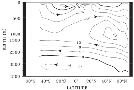
projections made with different state-of-the-art climate models. For example, Cubasch and Meehl (2001) compared projections of changes in the meridional overturning circulation in the North Atlantic from 10 different coupled atmosphere-ocean general circulation models (GCMs) for the same global warming scenario. This circulation is illustrated in Figure 1. The poleward flow near the surface is primarily associated with the Gulf Stream. This circulation is particularly important for climate, because it transports more heat than the circulations in any other ocean basin, and has a substantial warming effect on mid and high latitudes of the Northern Hemisphere (Seager et al., 2002). Estimates of the strength of the overturning circulation range from 16 to 25 Sv (Macdonald and Wunsch, 1996; Ganachaud, 2003; Sv = one Sverdrup = 106
m3
/s). However the simulated changes in this circulation by 2100 varied from no change to a decrease of 14 Sv. Since this result comes from coupled models, it is not possible to identify any single component of the climate system, such as the oceans, as being the source of the differences, without further analysis.
Figure 1. Typical model simulation of the stream function of the zonal mean overturning circulation in the North Atlantic. Depth is given on the vertical axis and latitude on the horizontal axis. Adapted from Huang et al. (2003).
An analysis which does implicate the ocean component of the climate models has been carried out by Sokolov et al. (2003). They found that model differences in projections of changes in global mean surface temperature could be attributed to differences in two model characteristics. One is the model’s climate sensitivity, defined as how much the global mean surface temperature would increase if the concentration of CO2 in the atmosphere were doubled and the climate system were allowed to equilibrate. This sensitivity depends primarily on atmospheric processes such as how clouds change when climate changes. These processes are not well understood and are represented in different ways in different models. The second model characteristic is the rate at which
perturbations in the heat flux between the atmosphere and ocean are mixed into the deep oceans.
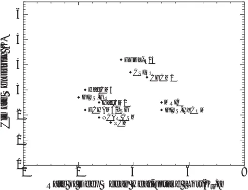
Figure 2 shows how 11 different coupled atmosphere-ocean GCMs differ with respect to
these two characteristics. In the figure, the rate of heat uptake by the deep oceans is measured by the global mean value of a coefficient which describes the effective rate at which heat anomalies are mixed into the deep ocean. In the figure the square root of this coefficient is plotted, since the depth to which heat penetrates at a given time is proportional to the square root of the coefficient. As shown in Figure 2, this depth varies between models by a factor of two and one half. The rate of heat uptake is not well constrained by the available observations (Forest et al., 2002), so none of these models can be ruled out by comparing them with the observations. Similarly we cannot be sure that any of them are right.
GFDL-R15 CGCM1 CSIRO
0 2 4 6 8
Rate of Deep Ocean Heat-uptake [Sqrt(Kv)] 0 1 2 3 4 5 6 Climate Sensitivity (K) GISS-GR HadCM2 ECHAM3/LSG NCAR CSM MRI1 HadCM3 PCM GISS-HYCOM
Figure 2. Properties of 11 different coupled GCMs. Vertical axis: climate sensitivity. Horizontal axis: a parameter measuring the depth to which heat has penetrated in the deep ocean (see text). Adapted from Sokolov et al. (2003).
One likely source of the ocean model differences in the rate of heat uptake is the different representations of small-scale oceanic processes used in different models. The differences reflect our ignorance of these processes, and this is one potential obstacle to our current ability to predict climate change. This problem will be discussed in Section 2.
Another potential obstacle is the possibility that the circulation in the North Atlantic and its heat transport may be very sensitive to small changes in climate. Since this circulation is coupled to that of the rest of the oceans by the “conveyor belt” circulation, such changes would have global consequences. Uncoupled ocean models that show this possibility include simple box models (Stommel, 1961; Rooth, 1982; Welander, 1986), two-dimensional meridional plane models (Marotzke et al., 1988), and three-dimensional numerical models (Bryan, 1986;
Marotzke and Willebrand, 1991). They all show that the circulation is very sensitive to salinity perturbations, particularly at high latitudes, and that the circulations can have at least two states. One is like that currently existing in the North Atlantic Ocean, with a relatively strong poleward heat transport. The other has a much weaker circulation with very little poleward heat transport.
Paleoclimatic evidence also indicates that two states like these with very different climates can exist (Broecker et al., 1985; Boyle and Keigwin, 1987; Broecker, 2003). Indeed, Broecker et al. (1985) suggest that sudden shifts in climate, such as that associated with the Younger Dryas event some 10,000 years ago, may have been caused by a sudden collapse in the circulation of the North Atlantic. How this phenomenon may limit predictions of climate change will be discussed in Section 3.
The limits on prediction described above could in principle be overcome if we could acquire data that is sufficiently extensive and accurate, and if our computers were sufficiently fast. However there may be a more fundamental limitation to our ability to predict changes in the oceans. The oceans’ circulations are highly nonlinear, but only weakly dissipative. Such systems are potentially chaotic, i.e., unpredictable past a certain time limit. This possibility will be discussed in Section 4. Finally, in Section 5, we will summarize our results and discuss possible paths for improving the predictions of ocean models and determining the limits of their
predictability.
2. SMALL-SCALE OCEANIC PROCESSES
The ocean GCMs used in current climate models have coarse resolution; typical horizontal resolutions are in the range 1° to 3°. Thus there are many subgrid-scale processes that need to be parameterized in these models. In current practice these processes are generally decomposed into four components which are parameterized separately: diapycnal diffusion, isopycnal diffusion, mesoscale eddies, and convection. Diapycnal diffusion refers to diffusion perpendicular to constant
density surfaces, while isopycnal diffusion refers to diffusion along constant density surfaces. Mesoscale eddies are eddies with typical spatial scales of about 100 km and typical periods of about 100 days. Energy spectra of the oceans show a peak at the frequency of the mesoscale eddies (Wunsch, 1981). The other parameterized processes occur at smaller spatial scales. There are major uncertainties and problems in current parameterizations of all these processes.
Diapycnal diffusion plays a particularly important role in determining the ocean’s circulation, since it is the diapycnal mixing of heat and salinity from the ocean’s surface into its depths that gives rise to the density gradients that drive the large-scale ocean circulation and its horizontal heat transports (Munk and Wunsch, 1998). In fact, scaling analyses and ocean GCM calculations show that the strength of the ocean circulations and heat transports are sensitive to the value of the diapycnal diffusion coefficient (Bryan, 1987; Marotzke, 1997). In a basin like the North Atlantic, the strength of the meridional overturning is approximately proportional to the 2/3 power of the coefficient and the poleward heat transport to the 1/2 power (Marotzke, 1997). The strength and heat transport are determined primarily by the values of the diapycnal diffusion at depths of 200 to 500 m in the tropics and subtropics (Scott and Martozke, 2002; Bugnion and Hill, 2003).
However OGCMs generally treat the diapycnal diffusion coefficients for heat, salinity, and momentum as constants, or as specified functions of depth. These representations are unlikely to be realistic. For example, one would expect the coefficients in general to depend on the shear and/or the stratification. Furthermore the values of the coefficients in the current climate are quite uncertain, with different measurements and estimates giving a range of 10–4
to 10–5 m2
/s (Munk and Wunsch, 1998). This is at least in part because they have strong spatial variations (e.g., Polzin et al., 1997).
OGCM calculations show that vertical mixing by the other three subgrid-scale processes is strongest in high latitudes (Huang et al., 2003a and 2003b). This is because the strong cooling of surface waters in high latitudes favors static instability and a vertical orientation of isopycnals. The former leads to convection; the latter leads both to isopycnal diffusion being predominantly vertical and to large amounts of potential energy being available for mesoscale eddies. The efficiency of all these processes is usually parameterized by specifying a constant diffusion coefficient.
The values of these coefficients are again poorly known. Estimates of the isopycnal diffusivity range from 500 to 2000 m2
/s (Hirst and Cai, 1994; Jenkins, 1991). The most popular parameterization of mesoscale eddies is the Gent-McWilliams parameterization, which requires the specification of both an isopycnal diffusion coefficient and a diffusion coefficient
parameterizing the effect of the mesoscale eddies on the density field (Gent and McWilliams, 1990). The two diffusivities are commonly (but arbitrarily) taken to be the same. Eddy-resolving
simulations show that in fact the mesoscale eddy diffusivity varies over a range of 10 to 107 m2
/s (Nakamura and Chao, 2000).
There are also theoretical reasons for questioning the adequacy of the parameterizations of high-latitude mixing. A fundamental limitation of the Gent-McWilliams parameterization is its assumption that mesoscale eddies’ energy source is potential energy, whereas eddy-resolving simulations show that the kinetic energy of the mean flow is also an important source of eddy energy (Solovev et al., 2002). In the case of parameterizations of convection, current schemes neglect the inhibiting effect of rotation on vertical motions (Marshall and Schott, 1999).
Finally we note that the calculation of the large-scale circulations in ocean GCMs is dependent on numerical schemes that are not perfect. Because of their inaccuracies there may be a significant amount of numerical diffusion, i.e., artificial mixing, in a model. Indeed it has been suggested that the unusually rapid mixing of heat into the deep ocean found in a global warming scenario with the GISS-HYCOM model (Sun and Bleck, 2001; Sokolov et al., 2003; see Figure 2) may be an artifact due to numerical diffusion in the HYCOM model (R. Bleck, personal communication).
3. STABILITY OF THE GLOBAL OCEAN CIRCULATION
As noted in the introduction, all ocean models show the possibility that the ocean circulation can be very sensitive to salinity perturbations and therefore to changes in surface freshwater fluxes. This sensitivity is closely associated with the fact that ocean models show the existence of more than one equilibrium state under some circumstances. These multiple equilibria arise because of a positive feedback associated with the advection of salinity in a circulation like that illustrated in Figure 1.
In this circulation the sinking is located in high latitudes, because that is where the surface waters are most dense. The density is a maximum there because the surface waters are coldest there. However the waters in high latitudes are relatively fresh compared to the subtropics because in high latitudes precipitation exceeds evaporation, while in the subtropics evaporation exceeds precipitation. Thus the poleward flow near the surface in a circulation like that shown in Figure 1 (basically the Gulf Stream) brings saltier water into high latitudes, and this tends to raise the density of the high latitude surface waters. Thus, this advection supplies a positive feedback to perturbations in the strength of the circulation. For example, if the circulation is weakened, the salinity advection weakens, the density of high latitude surface waters is decreased, and this weakens the circulation even more. Given a sufficiently strong initial
decrease in the circulation, it will collapse. As noted earlier, paleoclimate evidence does indicate that similar state changes have occurred in the past.
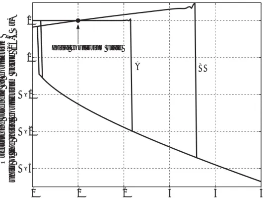
This behavior can be illustrated in a model by tracing out a hysteresis loop (Stocker and Wright, 1991; Rahmstorf, 1995a). Two such hysteresis loops, calculated with the Rooth (1982) box model, are shown in Figure 3. The equilibrium strength of the meridional overturning circulation in the Atlantic Ocean is plotted vs. the moisture flux into high latitudes of the North Atlantic, F1. A positive circulation means that there is a strong poleward heat flux into high latitudes of the North Atlantic, and, in this model, a weak poleward heat flux into high latitudes of the South Atlantic. A negative circulation implies the opposite. The former state is the one analogous to that of the Atlantic in the current climate.
As the figure shows, there is a range of values of the moisture flux where two equilibria exist. For smaller values of the moisture flux only the state with strong poleward heat flux in the North Atlantic can exist; for larger values of the moisture flux only the state with strong heat flux in the South Atlantic can exist. If the system is in the former state, a sufficiently large positive
perturbation added to the moisture flux will cause this state to collapse to the other equilibrium
0 1 2 3 4 5 –3 –2 –1 0 1
Overturning strength at equilibrium
units of the initial equilibriurm value (15.6 Sv)
F1 at equilibrium, units of the initial equilibrium value (0.40 Sv)
A B
Initial equilibrium state
Figure 3. Hysteresis loops calculated from the Rooth (1982) box model with mixed boundary conditions. Vertical axis: strength of the meridional overturning circulation in the Atlantic normalized by its value in the current climate. Horizontal axis: atmospheric moisture flux from low to high latitudes in the Northern Hemisphere, normalized by its value in the current climate. Curve A assumes that the atmospheric moisture flux in the Southern Hemisphere is kept fixed at its value in the current climate. Curve B assumes that Southern Hemisphere flux is increased from its current climate value by 20% of the increase in the Northern Hemisphere.
state, with a consequent large change in the oceanic heat transport and climate. How big a perturbation is required to accomplish this depends on many things. One factor is illustrated by the difference of the two hysteresis loops shown in Figure 2. Curve A is plotted under the
assumption that the moisture flux into high latitudes of the South Atlantic does not change when F1 changes. Curve B shows how the equilibrium state depends on F1 when there is a
simultaneous perturbation of the moisture flux into the high latitudes of the South Atlantic equal to 20% of F1. As the figure shows, increased moisture flux into southern high latitudes is a stabilizing influence, i.e., it takes larger perturbations in F1 to shift the system from one equilibrium state to the other.
A question of major importance to our understanding of the sensitivity of climate and its predictability is the question of where on the upper branch of the hysteresis loop the current climate is located. Ideally this question should be addressed with the most sophisticated state-of-the-art coupled GCMs. However to trace out such a curve with one of these models is not
computationally feasible. To do so requires either very many integrations with different values of F1, or a single integration in which F1 changes very slowly so that the model will evolve through the whole series of possible quasi-equilibrium states. This would require 10,000 or more years of integration, and no coupled GCM has yet been used to calculate such a hysteresis loop.
Recently however hysteresis loops for 11 different models of intermediate complexity have been calculated as part of an intercomparison project for earth models of intermediate
complexity (EMICs). EMICs are models which have less detail than state-of-the-art coupled GCMs, but do contain representations of all of the physical processes present in coupled GCMs, (Claussen et al., 2002). The results were reported at a workshop at the annual meeting of the European Geophysical Society in April, 2003. There was no agreement among the models as to the position of the current climate. All the models did have the position being on the upper branch of the hysteresis loop, as it has to be in order to be consistent with the modern climate, but the locations varied from being far to the left of the hysteresis loop, in the monostable regime, corresponding to a very stable climate, to the position being in the bistable region near the bifurcation at the right side of the loop, corresponding to a state with very weak stability.
Actually the situation appears to be even more complicated than is indicated by the simple hysteresis loops illustrated in Figure 3. EMICs with an ocean GCM and realistic ocean
bathymetry indicate the possibility of more than two equilibrium states, with the upper branch of the loop having a more complicated structure than that illustrated. In particular different states with somewhat different strengths for the overturning circulation are possible, depending on the sites of high latitude convection in the North Atlantic (Rahmstorf, 1995b).
The diversity of the model results for the state of the ocean circulation ultimately arises from the uncertainties in the input parameters for the climate models. One example is obvious from
Figure 3, i.e., one needs to know accurately the values of the freshwater flux into the high latitudes of the Atlantic Ocean. Since these fluxes depend on precipitation and evaporation over the oceans, where measurements are sparse, the errors are large, of order ±30% (Schmitt et al., 1989). In addition we note that the equilibrium states are not steady states, but rather contain fluctuations, presumably about a fixed climate state (see Section 4 and Figure 5 below). Also, if the climate forcing is not steady, as for example when greenhouse gases increase, the equilibrium states and the hysteresis loops will change.
Another major source of uncertainty involves again the uncertainty in small-scale oceanic mixing processes. Figure 4 illustrates two hysteresis loops calculated from an EMIC which includes an ocean GCM (Kamenkovich et al., 2002). In order to complete the calculations in a reasonable amount of time, the moisture flux into the North Atlantic was taken to evolve somewhat more rapidly than required for the plotted states to be precise equilibrium solutions,
0 0.1 0.2 0.3 0.4 0.5 0.6 0.7 0 5 10 15 20 25 30 Freshwater Forcing [Sv]
Maximum Overturning in the North Atlantic [Sv]
Figure 4. Hysteresis loops calculated with the MIT model of intermediate complexity (Kamenkovitch et al., 2002). Vertical axis: strength of the meridional overturning circulation in the North Atlantic.
Horizontal axis: moisture flux into the North Atlantic minus its value in the current climate. The states were traced out by starting with the current climate, then increasing the freshwater flux into the North Atlantic by 0.1 Sv/1000 years, and then after the circulation collapses, reversing the trend and returning to the current climate. The upper curve was calculated with a diapycnal diffusivity of 0.5 cm2/s, the lower one with 0.2 cm2/s. Adapted from Dalan (2003)
and thus the forward and return branches of the hysteresis loops do not coincide precisely. Note that in these calculations there was no change in the moisture flux into the South Atlantic, and that in Figure 4 on the horizontal axis is plotted the change in the moisture flux into the North Atlantic from that in the current climate, rather than the actual flux. The two hystersis loops were calculated for different values of the ocean model’s diapycnal diffusion coefficient, the upper one being for 0.5 cm2
/s, and the lower one for 0.2 cm2 /s.
As shown in the figure the hysteresis loops are displaced considerably from each other, and correspondingly the stability properties of the system are quite different, with the system being much less stable with the smaller value of the diffusivity. The intersection of the hysteresis curves with the vertical axis gives the strength of the overturning circulation in the North Atlantic in the current climate for the two values of the diapycnal diffusivity. Unfortunately, as we noted earlier, the strength is uncertain.
4. CHAOTIC BEHAVIOR
As noted in the introduction, oceanic circulations are likely to be chaotic, i.e., their evolution is likely to be very sensitive to the initial conditions. This behavior is well known in the
atmosphere, and has been studied extensively with atmospheric GCMs. The results show that weather cannot in principle be predicted more than about two weeks in advance because small errors in the initial conditions grow so rapidly. The dynamical time scales in the oceans are much longer than in the atmosphere, of order decades and centuries rather than days, and this makes it much more difficult computationally to assess how chaotic behavior may limit the predictability of ocean circulations. There have only been two studies using ocean GCMs which have
attempted to determine if such limits do exist. One by Griffies and Bryan (1997) (hereafter referred to as GB) looked at the predictability of fluctuations in the North Atlantic circulation; the other by Wang et al. (1999) (hereafter referred to as WSM) looked at the predictability of regime changes, i.e., of changes between different branches of the hysteresis loops discussed in the previous section.
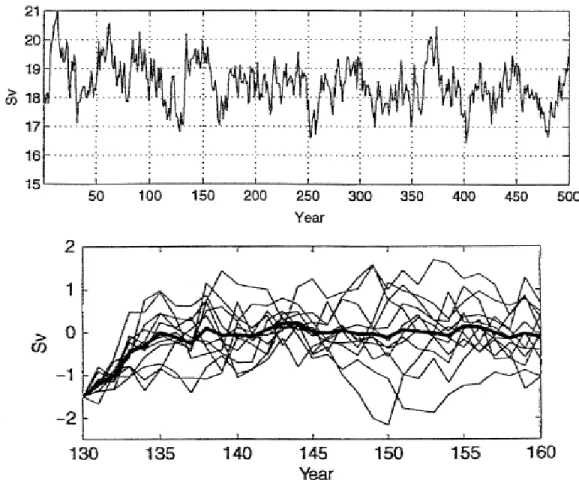
GB used a coupled atmosphere-ocean GCM in their study. They carried out a thousand-year integration with fixed forcing corresponding to the current climate. In this integration there were fluctuations in the strength of the meridional overturning circulation of the North Atlantic, as illustrated in the top of Figure 5. They then carried out an ensemble of 12 integrations in which the initial state of the oceans was taken from year 130 of the control run, but the initial state of the atmosphere varied, being picked from 12 different years in the control runs (but all from the same calendar date). Thus only the weather in the initial atmospheric state differed in the 12 runs. The results for the evolution of the strength of the meridional overturning circulation in the
Figure 5. Top: strength of the meridional overturning circulation in the North Atlantic vs. time from a 500-year segment of a control run with the GFDL coupled GCM. Bottom: same as the top figure, except the difference in the strength of the circulation from the mean of the control run is plotted on the vertical axis, and the results are taken from 12 different experiments, all starting from the oceanic state at year 130 in the control run, but with different initial conditions in the atmosphere. The thick line indicates the mean of the 12 experiments. Adapted from Griffies and Bryan (1997).
North Atlantic are shown in the bottom of Figure 5. We see that the ensemble members diverge, and GB found using a statistical test that there is some reasonable predictability of the circulation strength only for the first 3 years. This result is the oceanic analog (for this model) of the
prediction limit for atmospheric weather.
However from the point of view of climate, the GB result is not so relevant. The fluctuations in the circulation strength shown in Figure 5 are analogous to fluctuations in weather, and they all occur within the same climate regime. From the point of view of climate, a more interesting question is, what happens if the forcing changes? Is there a limit on our ability to predict regime changes? WSM examined this question using an ocean GCM with idealized global geometry. The ocean was forced by specified moisture fluxes and wind stresses, and the heat flux was calculated from a relaxation condition for the sea surface temperature. In the control run all these
boundary conditions were based on the current climate. In addition a stochastic forcing was added to the wind stress boundary condition in order to mimic atmospheric weather fluctuations.
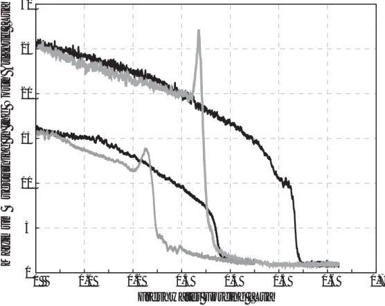
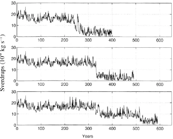
WSM then carried out an ensemble of runs in which the strength of the hydrological cycle in the Northern Hemisphere increased linearly, at a rate equal to 0.1% of the strength in the control run, per year. Thus the net precipitation in high latitudes of the Northern Hemisphere slowly increases and there is an equivalent increase in the net evaporation in low latitudes of the Northern Hemisphere. Three runs were carried out with three different choices for the initial value of the stochastic component of the wind stress. The results for the evolution of the strength of the meridional overturning circulation in the North Atlantic are shown in Figure 6.
Because of the very slow acceleration of the Northern Hemisphere hydrological cycle, the circulation evolves through a series of quasi-equilibrium states. In these equilibrium states the strength of the circulation does not change because the changes in precipitation and evaporation in the Northern Hemisphere in effect compensate each other. The increased precipitation in high latitudes reduces the density of the surface water there, but the increased evaporation in the
Figure 6. Strength of the meridional overturning circulation in the North Atlantic vs. time from 3 experiments with the WSM model in which the moisture flux into high latitudes of the North Atlantic slowly increased. The only difference between the experiments was the initial value of the atmospheric wind stress. Adapted from Wang et al. (1999).
subtropics increases the salinity of the subtropical surface waters, and this increases the
advection of salinity into high latitudes. The effect of the latter on the density of the high-latitude surface waters just balances the effect of the former, because there is no net exchange of
moisture between the atmosphere and ocean in the Northern Hemisphere as a whole. Thus the system evolves along a hysteresis loop like that shown by curve A in Figure 3.
During the initial phase of the experiments there are interannual fluctuations in the strength of the circulation which are comparable to those in the GB experiments (cf. Figures 5 and 6). However there is a striking difference in the nature of these fluctuations. In the WSM
experiments, the fluctuations in all three experiments are identical for about 200 years, i.e., the predictability time is much longer than in the GB experiments. One plausible reason for the difference is that the surface heat flux variations in the GB model were much larger and more realistic. Although GB found that the interannual variations in the ocean circulation were largely controlled by the internal ocean dynamics, surface heat fluxes did play a role, and their variations due to weather could have caused the loss of predictability compared to the WSM experiments. We note however that even the more realistic GB model has significant limitations. For example it has coarse horizontal resolution (~5°), which limits the ability to simulate realistic weather fluctuations, and the model can only reproduce the current climate by introducing large unphysical adjustments to the surface heat fluxes.
The more interesting aspect of the WSM experiments is what happened on the longer time scales. As discussed in the previous section the acceleration of the Northern Hemisphere
hydrological cycle must eventually lead to a collapse of the strong North Atlantic circulation (as indicated by curve A in Figure 3). It does in all three experiments but, as shown in Figure 6, the timing of the collapse, and the nature of the transition between the two circulation regimes differ considerably. Evidently the differences in the initial condition do not matter until the system approaches a bifurcation, and then there is a complete loss of predictability.
The two studies just described clearly only touch the surface of the problem of how prediction of changes in the ocean’s circulation may be limited by chaotic behavior. For example, it is not clear from these experiments whether fluctuations in the surface heat flux or wind stress are more important in limiting predictability in the ocean circulation on long time scales. In addition neither study looked at how the predictability is affected by perturbations in the initial state of the oceans.
5. POSSIBLE PATHS FORWARD
Forecasts of global warming during the 21st century indicate that the earth is likely to reach global temperatures higher than any it has experienced for at least 100,000 years (IPCC, 2001). This would take the earth to a situation outside the previous experience of our own species as
well as that of many others. Thus one of the most formidable scientific challenges facing society is the need to develop a better understanding of how the climate system operates and to predict, to the extent possible, the changes in climate and the environment that society must cope with in the future. Because of the great complexity of the climate system and the many different
disciplines that are required to deal with it, this is arguably the most difficult scientific task that has been undertaken. Because the natural response times of the ocean lie in the range of decades to centuries, understanding and predicting its behavior is essential for planning for the next few centuries.
In our discussion of the oceans we have focused on three problems which limit our ability to predict the ocean’s behavior. They are 1) our poor understanding of small-scale mixing
processes, 2) our inability to characterize the stability characteristics of the ocean circulation, and 3) the presence of chaotic elements in the ocean’s behavior. These problems are not independent. For example, the strength and behavior of the mixing properties affect the stability properties, and the stability properties influence the degree of chaotic behavior. In our discussion of the oceans, we focused on the North Atlantic because that is where ocean heat transports are strongest. However the circulations in the North Atlantic are not closed, but rather extend throughout the global oceans, as the “conveyor belt” circulation. Thus these problems are obstacles to understanding and modeling the whole global ocean. Because of these problems simulations of climate change with current state-of-the-art models are problematic.
With regard to the small-scale mixing processes, advances in computer speeds will
considerably alleviate at least the problems associated with parameterizations of mesoscale eddies. Since typical scales of these eddies are of order 100 km, models with horizontal resolutions of order 1/10 degree will have much less need to parameterize their effects. Such resolutions should be achievable for global climate models in the near future. Because oceanic energy spectra peak at the frequency of mesoscale eddies, this should mark a major advance in our models’ capabilities.
Unfortunately the other mixing processes occur on a much finer scale and thus ocean models will have to rely on subgrid-scale parameterizations for them for a long time to come. More observational estimates of vertical fluxes of heat and tracers, particularly in high latitudes, would be useful, but obtaining them is difficult and expensive. In this situation theoretical approaches may be the most fruitful. In particular one needs prognostic parameterizations rather than the empirical schemes based solely on the current climate that are commonly used in current ocean GCMs. One promising approach for improving current parameterizations is to use modern turbulence closure models to derive prognostic parameterizations (Canuto et al., 2001 and 2002).
However even these parameterizations still require the specification of the flux of energy into the oceans that drives the mixing. The major sources of this energy are believed to be surface winds and tidal mixing (Munk and Wunsch, 1998). Thus climate changes which lead to changes in
the surface winds might change the ocean mixing. Such an interaction has never been included in a climate model. Another potentially valuable step forward would be to couple these processes.
Because the stability characteristics of the ocean circulation depend on the small-scale mixing processes and surface flux climatologies (cf. Figures 3 and 4), improvements in our knowledge of both of these factors would help to determine the stability properties of the current climate. Paleoclimate data could also prove quite useful. There is considerable evidence indicating changes in the ocean’s circulation regime in the past (e.g., Broecker, 2003, and references therein) and these data could help constrain a fully coupled climate model to have the right stability properties.
The fundamental nature of the ocean’s circulations, i.e., their nonlinearity and weak
dissipation, make it inevitable that their behavior will contain some chaotic elements. Computers have played a prominent role in advancing our knowledge of chaotic behavior in other systems, and in principle they could also do so for the oceans. The primary obstacle so far has been the inherently long time scales associated with the oceans. However increases in computer speeds are now reaching the point where one can envisage carrying out ensembles of runs over long time scales with EMICS whose ocean component is an ocean GCM. Similar studies using coupled atmosphere-ocean GCMs are likely to be feasible within a decade or so. One key question that needs to be addressed is the question of whether the major sources of error growth are fluctuations in the ocean or in the atmosphere, and if the latter, which surface flux
fluctuations lead to the most rapid error growth. From the point of view of climate the key question that needs to be addressed is, to what extent does this error growth dominate over changes in forcing in controlling climate change?
Acknowledgments
I am indebted to Chris Forest for Figure 2, to Valerio Lucarini for Figure 3, to Fabio Dalan for Figure 4, and to Anne Slinn for Figures 1 and 6, and for formatting the other figures. Steve Sparks’ editorial advice led to significant improvements in the paper.
6. REFERENCES
Boyle, E. A., and L. Keigwin, North Atlantic thermohaline circulation during the past 20,000 years linked to high-latitude surface temperature, Nature, 330, 35-40, 1987.
Broecker, W., D. Peteet, and D. Rind, Does the ocean-atmosphere system have more than one stable mode of operation?, Nature, 315, 21-26, 1985.
Broecker, W. S., Does the trigger for abrupt climate change reside in the ocean or in the atmosphere?, Science, 300, 1519-1522, 2003.
Bryan, F., High-latitude salinity effects and interhemispheric thermohaline circulation, Nature, 323, 301-304, 1986.
Bryan, F., Parameter sensitivity of primitive equation ocean general circulation models, J. Phys. Oceanogr., 17, 970-985, 1987.
Bugnion, V., and C. Hill, The equilibration of an adjoint model on climatological time scales. Part II: Sensitivity of the thermohaline circulation to surface forcing and mixing in coupled and uncoupled models, J. Climate, submitted, 2003.
Canuto, V. M., A. Howard, Y. Cheng, and M. S. Dubovikov, Ocean turbulence: Part I: One-point closure model. Momentum and heat vertical diffusivities, J. Phys. Oceanogr., 31, 1313-1426, 2001.
Canuto, V. M., A. Howard, Y. Cheng, and M. S. Dubovikov, Ocean turbulence: Part II: Vertical diffusivities of momentum, heat, salt, mass and passive scalars, J. Phys. Oceanogr., 32, 240-264, 2002.
Claussen, M., et al., Earth system models of intermediate complexity : closing the gap in the spectrum of climate system models, Clim. Dyn., 18, 579-586.
Cubasch, U., and G. A. Meehl, Projections of future climate change. Climate Change 2002: the Scientific Basis, J. T. Houghton et al., eds., Cambridge University Press, Cambridge UK. Dalan, F., Sensitivity of climate change to diapycnal diffusivity in the ocean, Massachusetts
Institute of Technology M.S. thesis, Cambridge, MA, 96 pp., 2003.
Forest, C. E., P. H. Stone, A. P. Sokolov, M. R. Allen, and M. D. Webster, Quantifying uncertainties in climate system properties with the use of recent climate observations, Science, 295, 113-117, 2002.
Ganachaud, A., Large-scale mass transports, water mass formation, and diffusivities estimated from World Ocean Circulation Experiment, J. Geophys. Res., 108, No. C7, 3213, doi: 10.1029/2002JC001565, 2003.
Ganachaud, A., and C. Wunsch, Large-scale ocean heat and freshwater transports during the World Ocean Circulation Experiment, J. Climate, 16, 696-705, 2003.
Gent, P. R., and J. C. McWilliams, Isopycnal mixing in ocean circulation model, J. Phys. Oceanogr., 20, 150-155, 1990.
Griffies, S. M., and K. Bryan, A predictability study of simulated North Atlantic multidecadal variability, Clim. Dyn., 13, 459-487, 1997.
Hansen, J., G. Russell, A. Lacis, I. Fung, D. Rind, and P. Stone, Climate response times: dependence on climate sensitivity and ocean mixing, Science, 229, 857-859, 1985. Hirst, A., and W. Cai, Sensitivity of a world ocean GCM to changes in subsurface mixing
parameterization, J. Phys. Oceanogr., 24, 1256-1279, 1994.
Huang, B., P. H. Stone, and C. Hill, Sensitivities of deep-ocean heat uptake and heat content in an OGCM with idealized geometry, J. Geophys. Res., 108(C1), 3015, doi:10.1029/
Huang, B., P. H. Stone, A. P. Sokolov, and I. V. Kamenkovich, The deep-ocean heat uptake in transient climate change, J. Climate, 16, 1352-1363, 2003b.
IPCC, 2001: Climate Change 2001: The Scientific Basis (Houghton, J. T., et al., eds.), Cambridge University Press, Cambridge, UK, 881 pp.
Jenkins, W. J., Determination of isopycnal diffusivity in the Sargasso Sea, J. Phys. Oceanogr., 21, 1058-1061, 1991.
Kamenkovich, I. V., A. Sokolov, and P. H. Stone, An efficient climate model with a 3D ocean and statistical-dynamical atmosphere, Climate Dynamics, 19, 585-598, 2002.
Ledwell, J. R., E. T. Montgomery, K. L. Polzin, L. C. St. Laurent, R. W. Schmitt, and J. M. Toole, Evidence for enhanced mixing over rough topography in the abyssal ocean, Nature, 403, 79-182, 2000.
Levitus, S., J. I. Antonov, J. Wang, T. L. Delworth, K. W. Dixon, and A. J. Broccoli, Anthropogenic warming of earth’s climate system, Science, 292, 267-274, 2001.
Macdonald, A., and C. Wunsch, An estimate of global ocean circulation and heat fluxes, Nature, 382, 436-439, 1996.
Marotzke, J., P. Welander, and J. Willebrand, Instability and multiple steady states in a meridional-plane model of the thermohaline circulation, Tellus, 40A, 162-172, 1988. Marotzke, J., and J. Willebrand, Multiple equilibria of the global thermohaline circulation, J.
Phys. Oceanogr., 21, 1372-1385, 1991.
Marotzke, J., Boundary mixing and the dynamics of three-dimensional thermohaline circulations, J. Phys. Oceanogr., 27, 1713-1728, 1997.
Marshall, J., and F. Schott, Open-ocean convection: observations, theory and models, Revs. Geophys., 37, 1-64, 1999.
Munk, W., and C. Wunsch, Abyssal recipes II: energetics of tidal and wind mixing, Deep-Sea Res., 45, 1976-2009, 1998.
Nakamura, M., and Y. Chao, Characteristics of three-dimensional quasi-geostrophic transient eddy propagation in the vicinity of a simulated Gulf Stream, J. Geophys. Res., 105(C5) 11,385-11,406, 2000.
Rahmstorf, S., Bifurcations of the Atlantic thermohaline circulation in response to changes in the hydrological cycle, Nature, 378, 145-149, 1995a.
Rahmstorf, S., Multiple convection patterns and thermohaline flow in an idealized OGCM, J. Climate, 8, 3028-3039, 1995b.
Rooth, C., Hydrology and ocean circulation, Progress in Oceanography, 11, Pergamon, 131-149, 1982.
Schmitt, R. W., P. S. Bogden, and C. E. Dorman, Evaporation minus precipitation and density fluxes for the North Atlantic, J. Phys. Oceanogr., 19, 1208-1221, 1987.
Scott, J., and J. Marotzke, The location of diapycnal mixing and the meridional overturning circulation, J. Phys. Oceanogr., 32, 3578-3595, 2002.
Seager, R., D. S. Battisti, J. Yin, N. Gordon, N. Naik, A. C. Clement, and M. A. Cane, Is the Gulf Stream responsible for Europe’s mild winters?, Q. J. Roy. Met. Soc., 128 (586), 2563-2586, 2002.
Sokolov, A., C.E. Forest, and P. H. Stone, Comparing oceanic heat uptake in AOGCM transient climate change experiments, J. Climate, 16, 1573-1582, 2003.
Solovev, M., P. H. Stone, and P. Malanotte-Rizzoli: Assessment of mesoscale eddy parameterizations for a single basin coarse resolution ocean model, J. Geophys. Res., 107(C9), 9-1 - 9-19, doi:10.1029/2001JC001032, 2002.
Stocker, T. F., and D. G. Wright, Rapid transitions of the ocean’s deep circulation induced by changes in surface water fluxes, Nature, 351, 729-732, 1991.
Stommel, H., Thermohaline convection with two stable regimes of flow, Tellus, 13, 224-230, 1961.
Sun, S., and R. Bleck, Atlantic thermohaline circulation and its response to increasing CO2 in a coupled atmosphere-ocean model, Geophys. Res. Lett., 28, 4223-4226, 2001.
Trenberth, K. E., and J. M. Caron, Estimates of meridional atmosphere and ocean heat transports, J. Climate, 14, 3433-3443, 2001.
Wang, X., P. H. Stone, and J. Marotzke, Global thermohaline circulation, Part I: Sensitivity to atmospheric moisture transport, J. Climate, 12, 71-82, 1999.
Welander, P., Thermohaline effects in the ocean circulation and related simple models, Large-Scale Transport Processes in Oceans and Atmosphere, J. Willebrand and D. Anderson, eds., D. Reidel, 163-200, 1986.
Wunsch, C. Low-frequency variability of the sea, Evolution of Physical Oceanography, B. A. Warren and C. Wunsch, eds., MIT Press, 342-374, 1981.
REPORT SERIES of theMIT Joint Program on the Science and Policy of Global Change
1. Uncertainty in Climate Change Policy Analysis Jacoby & Prinn December 1994
2. Description and Validation of the MIT Version of the GISS 2D Model Sokolov & Stone June 1995
3. Responses of Primary Production & C Storage to Changes in Climate and Atm. CO2 Concentration Xiao et al. Oct 1995
4. Application of the Probabilistic Collocation Method for an Uncertainty Analysis Webster et al. January 1996 5. World Energy Consumption and CO2 Emissions: 1950-2050 Schmalensee et al. April 1996
6. The MIT Emission Prediction and Policy Analysis (EPPA) Model Yang et al. May 1996
7. Integrated Global System Model for Climate Policy Analysis Prinn et al. June 1996 (superseded by No. 36)
8. Relative Roles of Changes in CO2 & Climate to Equilibrium Responses of NPP & Carbon Storage Xiao et al. June 1996
9. CO2 Emissions Limits: Economic Adjustments and the Distribution of Burdens Jacoby et al. July 1997
10. Modeling the Emissions of N2O & CH4 from the Terrestrial Biosphere to the Atmosphere Liu August 1996
11. Global Warming Projections: Sensitivity to Deep Ocean Mixing Sokolov & Stone September 1996
12. Net Primary Production of Ecosystems in China and its Equilibrium Responses to Climate Changes Xiao et al. Nov 1996 13. Greenhouse Policy Architectures and Institutions Schmalensee November 1996
14. What Does Stabilizing Greenhouse Gas Concentrations Mean? Jacoby et al. November 1996 15. Economic Assessment of CO2 Capture and Disposal Eckaus et al. December 1996
16. What Drives Deforestation in the Brazilian Amazon? Pfaff December 1996
17. A Flexible Climate Model For Use In Integrated Assessments Sokolov & Stone March 1997
18. Transient Climate Change & Potential Croplands of the World in the 21st Century Xiao et al. May 1997 19. Joint Implementation: Lessons from Title IV’s Voluntary Compliance Programs Atkeson June 1997
20. Parameterization of Urban Sub-grid Scale Processes in Global Atmospheric Chemistry Models Calbo et al. July 1997 21. Needed: A Realistic Strategy for Global Warming Jacoby, Prinn & Schmalensee August 1997
22. Same Science, Differing Policies; The Saga of Global Climate Change Skolnikoff August 1997
23. Uncertainty in the Oceanic Heat and Carbon Uptake & their Impact on Climate Projections Sokolov et al. Sept 1997 24. A Global Interactive Chemistry and Climate Model Wang, Prinn & Sokolov September 1997
25. Interactions Among Emissions, Atmospheric Chemistry and Climate Change Wang & Prinn September 1997 26. Necessary Conditions for Stabilization Agreements Yang & Jacoby October 1997
27. Annex I Differentiation Proposals: Implications for Welfare, Equity and Policy Reiner & Jacoby October 1997 28. Transient Climate Change & Net Ecosystem Production of the Terrestrial Biosphere Xiao et al. November 1997 29. Analysis of CO2 Emissions from Fossil Fuel in Korea: 1961−1994 Choi November 1997
30. Uncertainty in Future Carbon Emissions: A Preliminary Exploration Webster November 1997
31. Beyond Emissions Paths: Rethinking the Climate Impacts of Emissions Protocols Webster & Reiner November 1997 32. Kyoto’s Unfinished Business Jacoby, Prinn & Schmalensee June 1998
33. Economic Development and the Structure of the Demand for Commercial Energy Judson et al. April 1998
34. Combined Effects of Anthropogenic Emissions & Resultant Climatic Changes on Atmosph. OH Wang & Prinn April 1998 35. Impact of Emissions, Chemistry, and Climate on Atmospheric Carbon Monoxide Wang & Prinn April 1998
36. Integrated Global System Model for Climate Policy Assessment: Feedbacks and Sensitivity Studies Prinn et al. June 1998 37. Quantifying the Uncertainty in Climate Predictions Webster & Sokolov July 1998
38. Sequential Climate Decisions Under Uncertainty: An Integrated Framework Valverde et al. September 1998 39. Uncertainty in Atmospheric CO2 (Ocean Carbon Cycle Model Analysis) Holian October 1998 (superseded by No. 80)
40. Analysis of Post-Kyoto CO2 Emissions Trading Using Marginal Abatement Curves Ellerman & Decaux October 1998
41. The Effects on Developing Countries of the Kyoto Protocol & CO2 Emissions Trading Ellerman et al. November 1998
42. Obstacles to Global CO2 Trading: A Familiar Problem Ellerman November 1998
43. The Uses and Misuses of Technology Development as a Component of Climate Policy Jacoby November 1998 44. Primary Aluminum Production: Climate Policy, Emissions and Costs Harnisch et al. December 1998
45. Multi-Gas Assessment of the Kyoto Protocol Reilly et al. January 1999
46. From Science to Policy: The Science-Related Politics of Climate Change Policy in the U.S. Skolnikoff January 1999 47. Constraining Uncertainties in Climate Models Using Climate Change Detection Techniques Forest et al. April 1999 48. Adjusting to Policy Expectations in Climate Change Modeling Shackley et al. May 1999
49. Toward a Useful Architecture for Climate Change Negotiations Jacoby et al. May 1999
50. A Study of the Effects of Natural Fertility, Weather & Productive Inputs in Chinese Agriculture Eckaus & Tso July 1999 51. Japanese Nuclear Power and the Kyoto Agreement Babiker, Reilly & Ellerman August 1999
52. Interactive Chemistry and Climate Models in Global Change Studies Wang & Prinn September 1999 53. Developing Country Effects of Kyoto-Type Emissions Restrictions Babiker & Jacoby October 1999 54. Model Estimates of the Mass Balance of the Greenland and Antarctic Ice Sheets Bugnion October 1999 55. Changes in Sea-Level Associated with Modifications of Ice Sheets over 21st Century Bugnion October 1999 56. The Kyoto Protocol and Developing Countries Babiker, Reilly & Jacoby October 1999
REPORT SERIES of theMIT Joint Program on the Science and Policy of Global Change
57. Can EPA Regulate GHGs Before the Senate Ratifies the Kyoto Protocol? Bugnion & Reiner November 1999 58. Multiple Gas Control Under the Kyoto Agreement Reilly, Mayer & Harnisch March 2000
59. Supplementarity: An Invitation for Monopsony? Ellerman & Sue Wing April 2000
60. A Coupled Atmosphere-Ocean Model of Intermediate Complexity Kamenkovich et al. May 2000 61. Effects of Differentiating Climate Policy by Sector: A U.S. Example Babiker et al. May 2000
62. Constraining Climate Model Properties Using Optimal Fingerprint Detection Methods Forest et al. May 2000 63. Linking Local Air Pollution to Global Chemistry and Climate Mayer et al. June 2000
64. The Effects of Changing Consumption Patterns on the Costs of Emission Restrictions Lahiri et al. August 2000 65. Rethinking the Kyoto Emissions Targets Babiker & Eckaus August 2000
66. Fair Trade and Harmonization of Climate Change Policies in Europe Viguier September 2000
67. The Curious Role of “Learning” in Climate Policy: Should We Wait for More Data? Webster October 2000 68. How to Think About Human Influence on Climate Forest, Stone & Jacoby October 2000
69. Tradable Permits for GHG Emissions: A primer with reference to Europe Ellerman November 2000 70. Carbon Emissions and The Kyoto Commitment in the European Union Viguier et al. February 2001
71. The MIT Emissions Prediction and Policy Analysis Model: Revisions, Sensitivities and Results Babiker et al. Feb 2001 72. Cap and Trade Policies in the Presence of Monopoly and Distortionary Taxation Fullerton & Metcalf March 2001 73. Uncertainty Analysis of Global Climate Change Projections Webster et al. March 2001 (superseded by No. 95) 74. The Welfare Costs of Hybrid Carbon Policies in the European Union Babiker et al. June 2001
75. Feedbacks Affecting the Response of the Thermohaline Circulation to Increasing CO2 Kamenkovich et al. July 2001
76. CO2 Abatement by Multi-fueled Electric Utilities: An Analysis Based on Japanese Data Ellerman & Tsukada July 2001
77. Comparing Greenhouse Gases Reilly, Babiker & Mayer July 2001
78. Quantifying Uncertainties in Climate System Properties using Recent Climate Observations Forest et al. July 2001 79. Uncertainty in Emissions Projections for Climate Models Webster et al. August 2001
80. Uncertainty in Atmospheric CO2 Predictions from a Global Ocean Carbon Cycle Model Holian et al. Sep 2001
81. A Comparison of the Behavior of AO GCMs in Transient Climate Change Experiments Sokolov et al. December 2001 82. The Evolution of a Climate Regime: Kyoto to Marrakech Babiker, Jacoby & Reiner February 2002
83. The “Safety Valve” and Climate Policy Jacoby & Ellerman February 2002
84. A Modeling Study on the Climate Impacts of Black Carbon Aerosols Wang March 2002 85. Tax Distortions and Global Climate Policy Babiker, Metcalf & Reilly May 2002
86. Incentive-based Approaches for Mitigating GHG Emissions: Issues and Prospects for India Gupta June 2002 87. Sensitivities of Deep-Ocean Heat Uptake and Heat Content to Surface Fluxes and Subgrid-Scale Parameters in an
Ocean GCM with Idealized Geometry Huang, Stone & Hill September 2002
88. The Deep-Ocean Heat Uptake in Transient Climate Change Huang et al. September 2002
89. Representing Energy Technologies in Top-down Economic Models using Bottom-up Info McFarland et al. Oct 2002 90. Ozone Effects on NPP and C Sequestration in the U.S. Using a Biogeochemistry Model Felzer et al. November 2002 91. Exclusionary Manipulation of Carbon Permit Markets: A Laboratory Test Carlén November 2002
92. An Issue of Permanence: Assessing the Effectiveness of Temporary Carbon Storage Herzog et al. December 2002 93. Is International Emissions Trading Always Beneficial? Babiker et al. December 2002
94. Modeling Non-CO2 Greenhouse Gas Abatement Hyman et al. December 2002
95. Uncertainty Analysis of Climate Change and Policy Response Webster et al. December 2002 96. Market Power in International Carbon Emissions Trading: A Laboratory Test Carlén January 2003
97. Emissions Trading to Reduce GHG Emissions in the US: The McCain-Lieberman Proposal Paltsev et al. June 2003 98. Russia’s Role in the Kyoto Protocol Bernard et al. June 2003
99. Thermohaline Circulation Stability: A Box Model Study Lucarini & Stone June 2003 100. Absolute vs. Intensity-Based Emissions Caps Ellerman & Sue Wing July 2003
101. Technology Detail in a Multi-Sector CGE Model: Transport Under Climate Policy Schafer & Jacoby July 2003 102. Induced Technical Change and the Cost of Climate Policy Sue Wing September 2003
103. Past and Future Effects of Ozone on Net Primary Production and Carbon Sequestration Using a Global Biogeochemical Model Felzer et al. October 2003 [Revised January 2004]
104. A Process-Based Modeling Analysis of Methane Exchanges Between Alaskan Terrestrial Ecosystems and the Atmosphere Zhuang et al. November 2003
105. Analysis of Strategies of Companies under Carbon Constraint: Relationship Between Profit Structure and
Carbon/Fuel Price Uncertainty Hashimoto January 2004