Relating Imprecise Representations of imprecise Probabilities

HAL Id: irsn-00196674

https://hal-irsn.archives-ouvertes.fr/irsn-00196674v2

Submitted on 2 Jan 2008

HAL is a multi-disciplinary open access

archive for the deposit and dissemination of

sci-entific research documents, whether they are

pub-lished or not. The documents may come from

teaching and research institutions in France or

abroad, or from public or private research centers.

L’archive ouverte pluridisciplinaire HAL, est

destinée au dépôt et à la diffusion de documents

scientifiques de niveau recherche, publiés ou non,

émanant des établissements d’enseignement et de

recherche français ou étrangers, des laboratoires

publics ou privés.

Relating Imprecise Representations of imprecise

Probabilities

Sébastien Destercke, Didier Dubois, Eric Chojnacki

To cite this version:

Sébastien Destercke, Didier Dubois, Eric Chojnacki. Relating Imprecise Representations of imprecise

Probabilities. fifth international symposium on imprecise probability: theories and applications, 2007,

Prague, Czech Republic. pp.155-165. �irsn-00196674v2�

5th International Symposium on Imprecise Probability: Theories and Applications, Prague, Czech Republic, 2007

Preprint of the paper presented at the ISIPTA 2007 conference

Relating practical representations of imprecise probabilities

Institut de Radioprotection et de Sûreté Nucléaire, DPAM, SEMIC, LIMSI,

Cadarache, France sebastien.destercke@irsn.fr

D. Dubois Institut de Recherche en Informatique de Toulouse (IRIT)

Toulouse, France dubois@irit.fr

E. Chojnacki Institut de Radioprotection

et de sûreté nucléaire, DPAM, SEMIC, LIMSI,

Cadarache, France eric.chojnacki@irsn.fr

Abstract

There exist many practical representations of prob-ability families that make them easier to handle. Among them are random sets, possibility distribu-tions, probability intervals, Ferson’s p-boxes and Neu-maier’s clouds. Both for theoretical and practical con-siderations, it is important to know whether one rep-resentation has the same expressive power than other ones, or can be approximated by other ones. In this paper, we mainly study the relationships between the two latter representations and the three other ones. Keywords. Random Sets, possibility distributions, probability intervals, p-boxes, clouds.

1

Introduction

There are many representations of uncertainty. When considering sets of probabilities as models of uncer-tainty, the theory of imprecise probabilities (includ-ing lower/upper previsions) [26] is the most general framework. It formally encompasses all the repsentations proposed by other uncertainty theories, re-gardless of their possible different interpretations. The more general the theory, the more expressive it can be, and, usually, the more expensive it is from a computational standpoint. Simpler (but less flexi-ble) representations can be useful if judged sufficiently expressive. They are mathematically and computa-tionally easier to handle, and using them can greatly increase efficiency in applications.

Among these simpler representations are random sets [7], possibility distributions [27], probability in-tervals [2], p-boxes [15] and, more recently, clouds [20, 21]. With such a diversity of simplified representa-tions, it is then natural to compare them from the standpoint of their expressive power. Building formal links between such representations also facilitates a unified handling of uncertainty, especially in propa-gation techniques exploiting uncertain data modeled

by means of such representations. This is the pur-pose of the present study. It extends some results by Baudrit and Dubois [1] concerning the relationships between p-boxes and possibility measures.

The paper is structured as follows: the first section briefly recalls the formalism of random sets, possibil-ity distributions and probabilpossibil-ity intervals, as well as some existing results. Section 3 then focuses on p-boxes, first generalizing the notion of p-boxes to arbi-trary finite spaces before studying the relationships of these generalized p-boxes with the three former rep-resentations. Finally, section 4 studies the relation-ships between clouds and the preceding representa-tions. For the reader convenience, longer proofs are put in the appendix.

2

Preliminaries

In this paper, we consider that uncertainty is modeled by a familyP of probability distributions, defined over a finite referential X = {x1, . . . , xn}. We also restrict

ourselves to families that can be represented by their lower and upper probability bounds, defined as fol-lows:

P(A) = inf

P ∈PP(A) and P (A) = sup_{P ∈P}P(A)

LetP_{P ,P} = {P |∀A ⊆ X, P (A) ≤ P (A) ≤ P (A)}. In general, we have P ⊂ P_{P ,P}, since P_{P ,P} can be seen as a projection of P on events. Although they are already restrictions from more general cases, dealing with families P_{P ,P} often remains difficult.

2.1 Random Sets

Formally, a random set is a mapping Γ from a prob-ability space to the power set ℘(X) of another space X, also called a multi-valued mapping. This map-ping induces lower and upper probabilities on X [7]. In the continuous case, the probability space is

of-ten [0, 1] equipped with Lebesgue measure, and Γ is a point-to-interval mapping.

In the finite case, these lower and upper probabili-ties are respectively called belief and plausibility mea-sures, and it can be shown that the belief measure is a ∞-monotone capacity [4]. An alternative (and useful) representation of the random set consists of a normal-ized distribution of positive masses m over the power set ℘(X) s.t. P_E⊆Xm(E) = 1 and m(∅) = 0 [24]. A set E that receives strict positive mass is said to be focal. Belief and plausibility functions are then defined as follows: Bel(A)=P E,E⊆Am(E) P l(A)=1−Bel(Ac₎₌P E,E∩A6=∅m(E). The set

PBel= {P |∀A ⊆ X, Bel(A) ≤ P (A) ≤ P l(A)}

is the probability family induced by the belief mea-sure.

Although 2|X| _{values are still needed to fully specify}

a general random set, the fact that they can be seen as probability distributions over subsets of X allows for simulation by means of some sampling process. 2.2 Possibility distributions

A possibility distribution π [12] is a mapping from X to the unit interval such that π(x) = 1 for some x ∈ X. Formally, a possibility distribution is the membership function of a fuzzy set. Several set-functions can be defined from a distribution π [11]:

• Π(A) = supx∈Aπ(x) (possibility measures);

• N (A) = 1 − Π(Ac_{) (necessity measures);}

• ∆(A) = infx∈Aπ(x) (sufficiency measures).

Possibility degrees express the extent to which an event is plausible, i.e., consistent with a possible state of the world, necessity degrees express the certainty of events and sufficiency (also called guaranteed possibil-ity) measures express the extent to which all states of the world where A occurs are plausible. They apply to so-called guaranteed possibility distributions [11] generally denoted by δ.

A possibility degree can be viewed as an upper bound of a probability degree [13]. Let

Pπ= {P, ∀A ⊆ X, N (A) ≤ P (A) ≤ Π(A)}

be the set of probability measures encoded by a pos-sibility distribution π. A pospos-sibility distribution is

also equivalent to a random set whose realizations are nested.

From a practical standpoint, possibility distributions are the simplest representation of imprecise probabil-ities (as for precise probabilprobabil-ities, only |X| values are needed to specify them). Another important point is their interpretation in term of collection of confidence intervals [10], which facilitates their elicitation and makes them natural candidate for vague probability assessments (see [5]).

2.3 Probability intervals

Probability intervals are defined as lower and up-per probability bounds restricted to singletons xi.

They can be seen as a collection of intervals L= {[li, ui], i = 1, . . . , n} defining a probability

fam-ily:

PL= {P |li≤ p(xi) ≤ ui∀xi∈ X}.

Such families have been extensively studied in [2] by De Campos et al.

In this paper, we consider non-empty families (i.e. PL6= ∅) that are reachable (i.e. each lower or upper

bound on singletons can be reached by at least one distribution of the family PL). Conditions of

non-emptiness and reachability respectively correspond to avoiding sure loss and achieving coherence in Walley’s behavioural theory.

Given intervals L, lower and upper probabilities P(A), P (A) are calculated by the following expres-sions

P(A) = max(P_xi∈Ali,1 −Pxi∈A/ ui)

P(A) = min(Pxi∈Aui,1 −

P

xi∈A/ li) (1)

De Campos et al. have shown that these bounds are Choquet capacities of order 2 ( P is a convex capac-ity).

The problem of approximating PL by a random set

has been treated in [17] and [8]. While in [17], Lem-mer and Kyburg find a random set m1 that is an

inner approximation of PL s.t. Bel1(xi) = li and

P l1(xi) = ui, Denoeux [8] extensively studies

meth-ods to build a random set that is an outer approxi-mation of PL. The problem of finding a possibility

distribution approximating PL is treated by Masson

and Denoeux in [19].

Two common cases where probability intervals can be encountered as models of uncertainty are confidence intervals on parameters of multinomial distributions built from sample data, and expert opinions providing such intervals.

3

P-boxes

We first recall some usual notions on the real line that will be generalized in the sequel.

Let Pr be a probability function on the real line with density p. The cumulative distribution of Pr is de-noted Fp _{and is defined by F}p_{(x) = Pr((−∞, x]).}

Let F1(x) and F2(x) be two cumulative distributions.

Then, F1(x) is said to stochastically dominate F2(x)

iff F1(x) ≤ F2(x) ∀x.

A P-box [15] is defined by a pair of cumulative distri-butions F ≤ F (F stochastically dominates F ) on the real line. It brackets the cumulative distribution of an imprecisely known probability function with density ps.t. F (x) ≤ Fp_{(x) ≤ F (x) ∀x ∈ <.}

3.1 Generalized Cumulative Distributions Interestingly, the notion of cumulative distribution is based on the existence of the natural ordering of num-bers. Consider a probability distribution (probability vector) λ = (λ1. . . λn) defined over the finite space

X; λi denotes the probability Pr(xi) of the i-th

ele-ment xi, and Pnj=1λj = 1. In this case, no natural

notion of cumulative distribution exists. In order to make sense of this notion over X, one must equip it with a complete preordering≤R, which is a reflexive,

complete and transitive relation. An R-downset is of the form{xi: xi≤Rx}, and denoted (x]R.

Definition 1. The generalized R-cumulative distribu-tion of a probability distribudistribu-tion on a finite, completely preordered set (X, ≤R) is the function FRλ: X → [0, 1]

defined by Fλ

R(x) = Pr((x]R).

The usual notion of stochastic dominance can also be defined for generalized cumulative distributions. Con-sider another probability distribution κ = (κ1. . . κn)

on X. The corresponding R-dominance relation of λ over κ can be defined by the pointwise inequality F_Rλ< F_Rκ. Clearly, a generalized cumulative distribu-tion can always be considered as a simple one, up to a reordering of elements.

Any generalized cumulative distribution Fλ

R with

re-spect to a complete preorder ≤R on X, of a

proba-bility measure Pr, with distribution λ on X, can also be used as a possibility distribution πR whose

asso-ciated measure dominates Pr, i.e. maxx∈AFRλ(x) ≥

Pr(A), ∀A ⊆ X. This is because a (generalized) cu-mulative distribution is constructed by computing the probabilities of events Pr(A) in a nested sequence of downsets (xi]R. [10].

3.2 Generalized p-box

Using the generalizations of the notions of cumulative distributions and of stochastic dominance described in section 3.1, we define a generalized p-box as follows Definition 2. A R-P-box on a finite, completely pre-ordered set (X, ≤R) is a pair of R-cumulative

distri-butions Fλ

R(x) and FRκ(x), s.t. FRλ(x) ≤ FRκ(x) (i.e. κ

is a probability distribution R-dominated by λ) The probability family induced by a R-P-box is

Pp−box= {P |∀x, FRλ(x) ≤ FR(x) ≤ FRκ(x).}

If we choose a relation R with xi ≤R xj iff i < j,

and, ∀xi ∈ X, consider the sets Ai = (xi]R, it

comes down to a family of nested confidence sets ∅ ⊆ A1 ⊆ A2 ⊆ . . . ⊆ An ⊂ X. The family Pp−box

can then be represented by the following restrictions on probability measures

αi≤ P (Ai) ≤ βi i= 1, . . . , n (2)

with α1 ≤ α2 ≤ . . . ≤ αn ≤ 1 and β1 ≤ β2 ≤ . . . ≤

βn ≤ 1. Choosing X = < and Ai = (−∞, xi], it is

easy to see that we find back the usual definition of P-boxes.

A generalized cumulative distribution being fully specified by |X| values, it follows that 2|X| values must be given to completely determine a generalized p-box. Moreover, we can interpret p-boxes as a col-lection of nested confidence intervals with upper and lower probability bounds (which could come, for ex-ample, from expert elicitation). In order to make no-tation simpler, the upper and lower cumulative distri-butions will respectively be noted F∗_{, F}

∗in the sequel

and, unless stated otherwise, we will consider (with-out loss of generality) the order R s.t. xi ≤R xj iff

i < j with the associated nested sets Ai. The notion

of generalized p-box is orthogonal to the notion of probability intervals in the sense that, in the former, probability bounds are assigned to a nested family of events, while for the latter, probability bounds are assigned to disjoint elementary events.

3.3 Generalized P-boxes in the setting of possibility theory

Given that sets Ai can be interpreted as nested

con-fidence intervals with upper and lower bounds, it is natural to search a connection with possibility the-ory, since possibility distributions can be interpreted as a collection of nested confidence intervals (a nat-ural way of expressing expert knowledge). We thus have the following proposition

Proposition 1. A familyPp−box described by a

gen-eralized P-box can be encoded by a pair of possibil-ity distributions π1, π2 s.t. Pp−box = Pπ1 ∩ Pπ2 with

π1(x) = F∗(x) and π2(x) = 1 − F∗(x)

Proof of proposition 1. Consider the definition of a generalized p-box and the fact that a generalized cumulative distribution can be used as a possibil-ity distribution πR dominating the probability

dis-tribution Pr (see section 3.1). Then, the set of con-straints (P (Ai) ≥ αi)i=1,n from equation (2)

gener-ates a possibility distribution π1 and the set of

con-straints (P (Ac

i) ≥ 1 − βi)i=1,n generates a possibility

distribution π2. ClearlyPp−box= Pπ₁∩ Pπ₂.

3.4 Generalized P-boxes are special case of random sets

The following proposition was proved in [9]

Proposition 2. A familyPp−box described by a

gen-eralized P-box can be encoded by a random set s.t. Pp−box = PBel.

Algorithm 1: R-P-box→ random set

Input: Nested sets∅, A1, . . . , An, X and bounds

αi, βi

Output: Equivalent random set fork= 1, . . . , n + 1 do

Build partition Fi = Ai\ Ai−1

Rank αi, βi increasingly

fork= 0, . . . , 2n + 1 do Rename αi, βi by γls.t.

α0= γ0= 0 ≤ γ1≤ . . . ≤ γl≤ . . . ≤ γ2n≤ 1 =

γ2n+1= βn+1

Define focal set E0= ∅

fork= 1, . . . , 2n + 1 do if γk−1= αithen Ek = Ek−1 ∪ Fi+1 if γk−1= βi then Ek = Ek−1 \ Fi Set m(Ek) = γk− γk−1

Algorithm 1 provides an easy way to build the ran-dom set encoding a generalized p-box. It is similar to algorithms given in [16, 23], and extends them to more general spaces. The main idea of the algorithm is to use the fact that a generalized p-box can be seen as a random set whose focal elements are unions of adjacent sets in a partition. Thanks to the nested na-ture of sets Ai, we can build a partition of X made

of Fi= Ai\ Ai−1, and then add or substract

consec-utive elements of this partition to build the focal sets (of the formS_j≤i≤kFi) of the random set equivalent

to the generalized p-box.

3.5 Generalized P-boxes and probability intervals

Provided an order R has been defined on elements xi,

a method to build a p-box from probability intervals L can be easily derived from equations (1). Lower an upper generalized cumulative distributions can be computed as follows F∗(xi) = P (Ai) = max( X xi∈Ai lj,1 − X xi∈A/ i uj) F∗(xi) = P (Ai) = min( X xi∈Ai ui,1 − X xi∈A/ i li) (3)

Transforming a p-box into probability intervals is also an easy task. First, let us assume that each element Fiof the partition used in algorithm 1 is reduced to a

singleton xi. Corresponding probability intervals are

then given by the two following formulas: P(Fi) = P (xi) = li= max(0, αi− βi−1)

P(Fi) = P (xi) = ui= βi− αi−1

if a set Fiis made of n elements xi1, . . . , xin, it is easy

to see that l(xij) = 0 and that u(xij) = P (Fi), since

xij ⊂ Fi.

Let us note that transforming probability intervals into p-boxes (and inversely) generally loses informa-tion, except in the degenerated cases of precise prability distribution and of total ignorance. If no ob-vious order relation R between elements xi is to be

privileged, and if one wants to transform probabil-ity intervals into generalized p-boxes, we think that a good choice for the order R is the one s.t.

n

X

i=1

F∗(xi) − F∗(xi)

is minimized, so that a minimal amount of informa-tion is lost in the process.

Another interesting fact to pinpoint is that both cu-mulative distributions given by equations (3) can be interpreted as possibility distributions dominating the familyPL (for F∗, the associated possibility

distribu-tion is 1 − F∗). Thus, computing either F∗ or F∗ is a

method to find a possibility distribution approximat-ing PL, which is different from the one proposed by

Masson and Denoeux [19].

4

Clouds

We begin this section by recalling basic definitions and results due to Neumaier [20], cast in the ter-minology of fuzzy sets and possibility theory. A

cloud is an Interval-Valued Fuzzy Set F such that (0, 1) ⊆ ∪x∈XF(x) ⊆ [0, 1], where F (x) is an interval

[δ(x), π(x)]. In the following, it is either defined on a finite space X, or it is a continuous interval-valued fuzzy interval (IVFI) on the real line ( a “cloudy” inter-val). In the latter case each fuzzy set has cuts that are closed intervals. When the upper membership func-tion coincides with the lower one, (δ = π) the cloud is called thin, and when the lower membership function is identically 0, the cloud is called fuzzy by Neumaier. Let us note that these names are somewhat counter-intuitive, since a thin cloud correspond to a fuzzy set with precise membership function, while a fuzzy cloud is equivalent to a probability family modeled by a pos-sibility distribution.

A random variable x with values in X is said to belong to a cloud F if and only if∀α ∈ [0, 1]:

P(δ(x) ≥ α) ≤ 1 − α ≤ P (π(x) > α) (4) under all suitable measurability assumptions. If X is a finite space of cardinality n, a cloud can be defined by the following restrictions :

P(Bi) ≤ 1 − αi≤ P (Ai) and Bi⊆ Ai, (5)

where 1 = α0 > α1 > α2 > . . . > αn > αn+1 = 0

and ∅ = A0 ⊂ A1 ⊆ A2 ⊆ . . . ⊆ An ⊆ An+1 =

X; ∅ = B0 ⊆ B1 ⊆ B2 ⊆ . . . ⊆ Bn ⊆ Bn+1 = X.

The confidence sets Ai and Bi are respectively the

strong and regular α-cut of fuzzy sets π and δ (Ai =

{xi, π(xi) > αi+1} and Bi= {xi, δ(xi) ≥ αi+1}).

As for probability intervals and p-boxes, eliciting a cloud requires 2|X| values.

4.1 Clouds in the setting of possibility theory

Let us first recall the following result regarding possi-bility measures (see [10]):

Proposition 3. P ∈ Pπ if and only if 1 − α ≤

P(π(x) > α), ∀α ∈ (0, 1]

The following proposition directly follows

Proposition 4. A probability family Pδ,π described

by the cloud (δ, π) is equivalent to the family Pπ ∩

P1−δ described by the two possibility distributions π

and 1 − δ.

Proof of proposition 4. Consider a cloud (δ, π), and define π = 1−δ. Note that P (δ(x) ≥ α) ≤ 1−α is equivalent to P (π > β) ≥ 1 − β, letting β = 1 − α. So it is clear from equation (4) that probability measure P is in the cloud (δ, π) if and only if it is in Pπ∩ Pπ.

So a cloud is a family of probabilities dominated by two possibility distributions (see [14]) .

0 1 π δ A₁ A2 A₃ B₁ B₂ B3 α1 α2 α3

Figure 1: Comonotonic cloud

0 1 π δ A1 A₂ A₃ B₂ B₃ α1 α2 α3

Figure 2: Non-Comonotonic cloud

This property is common to generalized p-boxes and clouds: they define probability families upper bounded by two possibility measures. It is then nat-ural to investigate their relationships.

4.2 Finding clouds that are generalized p-boxes

Proposition 5. A cloud is a generalized p-box iff {Ai, Bi, i = 1, . . . , n} form a nested sequence of sets

(i.e. there is a linear preordering with respect to in-clusion)

Proof of proposition 5. Assume the sets Ai and

Bj form a globally nested sequence whose current

el-ement is Ck. Then the set of constraints defining a

cloud can be rewritten in the form γk ≤ P (Ck) ≤ βk,

where γk= 1 − αiand βk = min{1 − αj : Ai ⊆ Bj} if

Ck= Ai; βk = 1−αiand γk= max{1−αj: Aj⊆ Bi}

if Ck= Bi.

Since 1 = α0 > α1 > . . . > αn < αn+1 = 0, these

constraints are equivalent to those of a generalized p-box. But if ∃ Bj, Ai with j > i s.t. Bj 6⊂ Ai and

Ai6⊂ Bj, then the cloud is not equivalent to a p-box,

since confidence sets would no more form a complete preordering with respect to inclusion.

In term of pairs of possibility distributions, it is now easy to see that a cloud (δ, π) is a generalized p-box if and only if π and δ are comonotonic. We will thus call such clouds comonotonic clouds. If a cloud is comonotonic, we can thus directly adapt the various results obtained for generalized p-boxes. In

partic-ular, because comonotonic clouds are generalized p-boxes, algorithm 1 can be used to get the correspond-ing random set. Notions of comonotonic and non-comonotonic clouds are respectively illustrated by fig-ures 1 and 2

4.3 Characterizing and approximating non-comonotonic clouds

The following proposition characterizes probability families represented by most non-comonotonic clouds, showing that the distinction between comonotonic and non-comonotonic clouds makes sense (since the latter cannot be represented by random sets). Proposition 6. If (δ, π) is a non-comonotonic cloud for which there are two overlapping sets Ai, Bj that

are not nested (i.e. Ai∩ Bj 6= {Ai, Bj,∅}), then the

lower probability of the induced familyPδ,πis not even

2-monotone.

and the proof can be found in the appendix.

Remark 1. The case for which we have Bj∩ Ai ∈

{Ai, Bj} for all pairs Ai, Bj is the case of

comono-tonic clouds. Now, if a cloud is such that for all pairs Ai, Bj : Bj∩ Ai∈ {Ai, Bj,∅} with at least one empty

intersection, then it is still a random set, but no longer a generalized p-box. Let us note that this special case can only occur for discrete clouds.

Since it can be computationally difficult to work with capacities that are not 2-monotone, one could wish to work either with outer or inner approximations. We propose two such approximations, which are easy to compute and respectively correspond to necessity (possibility) measures and belief (plausibility) mea-sures.

Proposition 7. If Pδ,π is the probability family

de-scribed by the cloud (δ, π) on a referential X, then, the following bounds provide an outer approximation of the range of P (A) :

max(Nπ(A), N1−δ(A)) ≤ P (A) ≤

min(Ππ(A), Π1−δ(A)) ∀A ⊂ X (6)

Proof of proposition 7. Since we have thatPδ,π=

P1−δ∩ Pπ, and given the bounds defined by each

pos-sibility distributions, it is clear that equation 6 give bounds of P (A).

Nevertheless, these bounds are not, in general, the infinimum and the supremum of P (A) over Pδ,π. To

see this, consider a discrete cloud made of four

non-empty elements A1, A2, B1, B2. It can be checked that

π(x) = 1 if x ∈ A1; = α1 if x∈ A2\ A1; = α2if x6∈ A2. δ(x) = α1 if x∈ B1; = α2 if x∈ B2\ B1; = 0 if x 6∈ B2. Since P (A2) ≥ 1 − α2 and P (B1) ≤ 1 − α1,

from (5), we can easily check that P (A2 \ B1) =

P(A2 ∩ Bc1) = α1 − α2. Now, Nπ(A2 ∩ B1c) =

min(Nπ(A2), Nπ(Bc1)) = 0 since Ππ(B1) = 1 because

B1 ⊆ A1. Considering distribution δ, we can have

N1−δ(A2 ∩ B1c) = min(N1−δ(A2), N1−δ(B1c)) = 0

since N1−δ(A2) = ∆δ(Ac2) = 0 since B2 ⊆ A2.

Equation (6) can thus result in a trivial lower bound, different from P (A2\ B1).

We can check that the bounds given by equation (6) are the one considered by Neumaier in [20]. Since these bounds are, in general, not the infinimum and supremum of P (A) on Pδ,π, Neumaier’s claim that

clouds are only vaguely related to Walley’s previsions or random sets is not surprising. Nevertheless, if we consider the relationship between clouds and possi-bility distributions, taking this outer approximation, that is very easy to compute, seems very natural. The next proposition provides an inner approximation of Pδ,π

Proposition 8. Given the sets{Bi, Ai, i= 1, . . . , n}

constituting the distributions (δ, π) of a cloud and the corresponding αi, the belief and plausibility measures

of the random set s.t. m(Ai\ Bi−1) = αi−1− αi are

inner approximations of Pδ,π.

It is easy to see that this random set can always be defined. We can see that it is always an inner approx-imation by using the contingency matrix advocated in the proof of proposition 6 (see appendix). In this matrix, the random set defined above comes down to concentrating weights on diagonal elements.

This inner approximation is exact in case of comono-tonicity or when we have Ai∩Bj∈ {Ai, Bj,∅} for any

pair of sets Ai, Bj defining the clouds.

4.4 A note on thin and continuous clouds Thin clouds (δ = π) constitute an interesting special case of clouds. In this latter case, conditions defining clouds are reduced to

On finite sets these constraints are generally contra-dictory, because P (π(x) ≥ α) > P (π(x) > α) for some α, hence the following theorem:

Proposition 9. If X is finite, then P(π) ∩ P(1 − π) is empty.

which is proved in [14], where it is also shown that this emptiness is due to finiteness. A simple shift of indices solves the difficulty. Let π(ui) = αi such that

α1 = 1 > . . . > αn > αn+1 = 0. Consider δ(ui) =

αi+1 < π1(ui). Then P(π) ∩ P(1 − δ) contains the

unique probability measure P such that the probabil-ity weight attached to uiis pi= αi−αi+1,∀i = 1 . . . n.

To see it, refer to equation (5), and note that in this case Ai= Bi.

In the continuous case, a thin cloud is non-trivial. The inclusions [δ(x) ≥ α] ⊆ [π(x) > α] (correspond-ing to Bi ⊆ Ai) again do not work but we may have

P(π(x) ≥ α) = P (π(x) > α) = 1 − α, ∀α ∈ (0, 1). For instance, a cumulative distribution function, viewed as a tight p-box, defines a thin cloud containing the only random variable having this cumulative distribu-tion (the “right” side of the cloud is rejected to∞). In fact, it was suggested in [14] that a thin cloud contains in general an infinity of probability distributions. Insofar as Proposition 5 can be extended to the re-als (this could be shown, for instance, by proving the convergence of some finite outer and inner approxima-tions of the continuous model, or by using the notion of directed set [5] to prove the complete monotonic-ity of the model), then a thin cloud can be viewed as a generalized p-box and is thus a (continuous ) be-lief function with uniform mass density, whose focal sets are doubletons of the form {x(α), y(α)} where {x : π(x) ≥ α} = [x(α), y(α)]. It is defined by the Lebesgue measure on the unit interval and the mul-timapping α−→ {x(α), y(α)}. This result gives us a nice way to characterize the infinite quantity of ran-dom variables contained in a thin cloud. In particular, concentrating the mass density on elements x(α) or on elements y(α) would respectively give the upper and lower cumulative distributions that would have been associated to the possibility distribution π alone (let us note that every convex mixture of those two cumu-lative distributions would also be in the thin cloud). It is also clear that Bel(π(x) ≥ α) = 1 − α. More gen-erally, if Proposition 5 holds in the continuous case, a comonotonic cloud can be characterized by a contin-uous belief function [25] with uniform mass density, whose focal sets would be disjoint sets of the form [x(α), u(α)] ∪ [v(α), y(α)] where {x : π(x) ≥ α} = [x(α), y(α)] and {x : δ(x) ≥ α} = [u(α), v(α)].

4.5 Clouds and probability intervals

Since probability intervals are 2-monotone capacities, while clouds are either∞-monotone capacities or not even 2-monotone capacities, there is no direct corre-spondence between probability intervals and clouds. Nevertheless, given previous results, we can easily build a cloud approximating a family PL defined by

a set L of probability intervals (but perhaps not the most "specific" one): indeed, any generalized p-box built from the probability intervals is a comonotonic cloud encompassing the familyPL.

Although finding the "best" (i.e. keeping as much information as possible, given some information mea-sure) method to transform probability intervals into cloud is an open problem. Any such transformation should follow some basic requirements such as:

1. Since clouds can model precise probability distri-butions, the method should insure that a precise probability distribution will be transformed into the corresponding thin cloud.

2. Given a set L of probability intervals, the trans-formed cloud [δ, π] should contain PL (i.e. Pδ,π,

while being as close to it as possible. ⊂ PL).

Let us note that using the transformation proposed in section 3.5 for generalized p-boxes satisfies these two requirements. Another solution is to extend Mas-son and Denoeux’s [19] method that builds a possibil-ity distribution covering a set of probabilpossibil-ity intervals, completing it by a lower distribution δ (due to lack of space, we do not explore this alternative here).

5

Conclusions

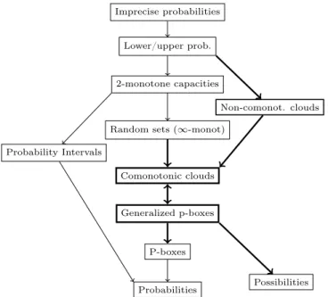
Figure 3 summarizes our results cast in a more gen-eral framework of imprecise probability representa-tions (our main contriburepresenta-tions in boldface).

In this paper, we have considered many practical rep-resentations of imprecise probabilities, which are eas-ier to handle than general probability families. They often require less data to be fully specified and they allow many mathematical simplifications, which may prove to increase computational efficiency (except, perhaps, for non-comonotonic clouds).

Some clarifications have been brought concerning the properties of the cloud formalism. The fact that non-comonotonic clouds are not even 2-monotone capac-ities tends to indicate that, from a computational standpoint, they sound less interesting than the other formalisms. Nevertheless, as far as we know, they are the only simple model generating capacities that are not 2-monotone.

Imprecise probabilities

Lower/upper prob.

2-monotone capacities

Random sets (∞-monot)

Comonotonic clouds Generalized p-boxes P-boxes Probabilities Probability Intervals Non-comonot. clouds Possibilities

Figure 3: Representations relationships. A−→ B : B is a special case of A

A work that remains to be done to a large ex-tent is to evaluate the validity and the usefulness of these representations, particularly from a psycholog-ical standpoint (even if some of it has already been done [22, 18]). Another issue is to extend presented results to continuous spaces or to general lower/upper previsions (by using results from, for example [25, 6]). Finally, a natural continuation to this work is to ex-plore various aspects of each formalisms in a manner similar to the one of De campos et al. [2]. What be-comes of random sets, possibility distributions, gen-eralized p-boxes and clouds after fusion, marginaliza-tion, conditioning or propagation? Do they preserve the representation? and under which assumptions ? To what extent are these representations informative ? Can they easily be elicited or integrated ? If many results already exist for random sets and possibility distributions, there are fewer results for generalized p-boxes or clouds, due to their novelty.

Acknowledgements

This paper has been supported by a grant from the Institut de Radioprotection et de Sûreté Nucléaire (IRSN). Scientific responsibility rests with the au-thors.

References

[1] C. Baudrit and D. Dubois. Practical rep-resentations of incomplete probabilistic

knowl-edge. Computational Statistics and Data Anal-ysis, 51(1):86–108, 2006.

[2] L. de Campos, J. Huete, and S. Moral. Probabil-ity intervals : a tool for uncertain reasoning. I. J. of Uncertainty, Fuzziness and Knowledge-Based Systems, 2:167–196, 1994.

[3] A. Chateauneuf. Combination of compatible belief functions and relation of specificity. In Advances in the Dempster-Shafer theory of ev-idence, pages 97–114. John Wiley & Sons, Inc, New York, NY, USA, 1994.

[4] G. Choquet. Theory of capacities. Annales de l’institut Fourier, 5:131–295, 1954.

[5] G. de Cooman. A behavioural model for vague probability assessments. Fuzzy sets and systems, 154:305–358, 2005.

[6] G. de Cooman, M. Troffaes, and E. Miranda. n-monotone lower previsions and lower integrals. In F. Cozman, R. Nau, and T. Seidenfeld, editors, Proc. 4th International Symposium on Imprecise Probabilities and Their Applications, 2005. [7] A. Dempster. Upper and lower probabilities

in-duced by a multivalued mapping. Annals of Mathematical Statistics, 38:325–339, 1967. [8] T. Denoeux. Constructing belief functions from

sample data using multinomial confidence re-gions. I. J. of Approximate Reasoning, 42, 2006. [9] S. Destercke and D. Dubois. A unified view of some representations of imprecise probabilities. In J. Lawry, E. Miranda, A. Bugarin, and S. Li, editors, Int. Conf. on Soft Methods in Probability and Statistics (SMPS), Advances in Soft Com-puting, pages 249–257, Bristol, 2006. Springer. [10] D. Dubois, L. Foulloy, G. Mauris, and H. Prade.

Probability-possibility transformations, triangu-lar fuzzy sets, and probabilistic inequalities. Re-liable Computing, 10:273–297, 2004.

[11] D. Dubois, P. Hajek, and H. Prade. Knowledge-driven versus data-Knowledge-driven logics. Journal of logic, Language and information, 9:65–89, 2000. [12] D. Dubois and H. Prade. Possibility Theory : An

Approach to Computerized Processing of Uncer-tainty. Plenum Press, 1988.

[13] D. Dubois and H. Prade. When upper proba-bilities are possibility measures. Fuzzy Sets and Systems, 49:65–74, 1992.

[14] D. Dubois and H. Prade. Interval-valued fuzzy sets, possibility theory and imprecise probabil-ity. In Proceedings of International Conference in Fuzzy Logic and Technology (EUSFLAT’05), Barcelona, September 2005.

[15] S. Ferson, L. Ginzburg, V. Kreinovich, D. Myers, and K. Sentz. Construction probability boxes and dempster-shafer structures. Technical re-port, Sandia National Laboratories, 2003. [16] E. Kriegler and H. Held. Utilizing belief functions

for the estimation of future climate change. I. J. of Approximate Reasoning, 39:185–209, 2005. [17] J. Lemmer and H. Kyburg. Conditions for the

existence of belief functions corresponding to in-tervals of belief. In Proc. 9th National Conference on A.I., pages 488–493, 1991.

[18] G. N. Linz and F. C. de Souza. A protocol for the elicitation of imprecise probabilities. In Proceed-ings 4th International Symposium on Imprecise Probabilities and their Applications, Pittsburgh, 2005.

[19] M. Masson and T. Denoeux. Inferring a possibil-ity distribution from empirical data. Fuzzy Sets and Systems, 157(3):319–340, february 2006. [20] A. Neumaier. Clouds, fuzzy sets and probability

intervals. Reliable Computing, 10:249–272, 2004. [21] A. Neumaier. On the structure of clouds.

avail-able on www.mat.univie.ac.at/∼neum, 2004. [22] E. Raufaste, R. Neves, and C. Mariné. Testing

the descriptive validity of possibility theory in human judgments of uncertainty. Artificial In-telligence, 148:197–218, 2003.

[23] H. Regan, S. Ferson, and D. Berleant. Equiva-lence of methods for uncertainty propagation of real-valued random variables. I. J. of Approxi-mate Reasoning, 36:1–30, 2004.

[24] G. Shafer. A mathematical Theory of Evidence. Princeton University Press, 1976.

[25] P. Smets. Belief functions on real numbers. I. J. of Approximate Reasoning, 40:181–223, 2005. [26] P. Walley. Statistical reasoning with imprecise

Probabilities. Chapman and Hall, 1991.

[27] L. Zadeh. Fuzzy sets as a basis for a theory of possibility. Fuzzy sets and systems, 1:3–28, 1978.

Appendix

Proof of proposition 6 (sketch). Our proof uses the following result by Chateauneuf [3]: Let m1,m2

be two random sets with focal sets F1,F2, each

of them respectively defining a probability family PBel₁,PBel₂. Here, we assume that those families are

"compatible" (i.e. PBel₁∩ PBel₂ 6= ∅).

Then, the result from Chateauneuf states the follow-ing : the lower probability P (E) of the event E on PBel1 ∩ PBel2 is equal to the least belief measure

Bel(E) that can be computed on the set of joint nor-malized random sets with marginals m1,m2. More

formally, let us consider a set Q s.t. Q ∈ Q iff

• Q(A, B) > 0 ⇒ A × B ∈ F1× F2 (masses over

the cartesian product of focal sets)

• A ∩ B = ∅ ⇒ Q(A, B) = 0 (normalization con-straints)

• m_P1(A) = PB∈F₂Q(A, B) and m2(B) = A∈F₁Q(A, B) (marginal constraints)

and the lower probability P (E) is given by the follow-ing equation P(E) = min Q∈Q X (A∩B)⊆E Q(A, B) (7)

where Q is the set of joint normalized random sets. This result can be applied to clouds, since the family described by a cloud is the intersection of two families modeled by possibility distributions.

To illustrate the general proof, we will restrict our-selves to a 4-set cloud (the most simple non-trivial cloud that can be found). We thus consider four sets A1, A2, B1, B2 s.t. A1 ⊂ A2,B1 ⊂ B2,Bi ⊂ Ai

to-gether with two values α1, α2 s.t. 1(= α0) > α1 >

α2 >0(= α3) and the cloud is defined by enforcing

the inequalities P (Bi) ≤ 1 − αi≤ P (Ai) i = 1, 2. The

random sets equivalent to the possibility distributions π,1 − δ are summarized in the following table:

π 1 − δ

m(A1) = 1 − α1 m(B0c= X) = 1 − α1

m(A2) = α1− α2 m(Bc1) = α1− α2

m(A3= X) = α2 m(B2c) = α2

Furthermore, we add the constraint A1 ∩ B2 6=

{A1, B2,∅}, related to the non-monotonicity of the

cloud. We then have the following contingency ma-trix, where the mass mij is assigned to the

iand the top of column j: B0c= X B1c B2c P A1 m11 m12 m13 1 − α1 A2 m21 m22 m23 α1− α2 A3_P= X m31 m32 m33 α2 1 − α1 α1− α2 α2 1

We now consider the four events A1, B2c, A1∩ Bc2, A1∪

B₂c. Given the above contingency matrix, we imme-diately have P (A1) = 1 − α1 and P (B2c) = α2, since

A1 only includes the (joint) focal sets in the first line

and Bc

2 in the third column.

It is also easy to see that P (A1∩ B2c) = 0, by

consid-ering the mass assignment mii = αi−1− αi (we then

have m13= 0, which is the mass of the only joint focal

set included in A1∩ B2c).

Now, concerning P (A1∪ B2c), let us consider the

fol-lowing mass assignment:

m22= α1− α2

m31= min(1 − α1, α2)

m11= 1 − α1− m31

m33= α2− m31

m13= m31

it can be checked that this mass assignment satisfies the constraints of the contingency matrix, and that the only joint focal sets included in A1∪ Bc2are those

with masses m11, m33, m13. Summing these masses,

we have P (A1∪ B2c) = max(α2,1 − α1). Hence:

P(A1∪ B2c) + P (A1∩ Bc2) < P(B2c) + P (A1)

max(α2,1 − α1) < 1 − α1+ α2

an inequality that clearly violates the 2-monotonicity property. We have thus shown that in the 4-set case, 2-monotonocity never holds for families modeled by non-comonotonic clouds.

Now, in the general case, we have the following con-tingency matrix B0c · Bcj · Bnc P A1 m11 1 − α1 · · Ai mi(j+1) αi−1− αi · · A_Pn+1 m(n+1)(n+1) αn 1− αj− αn α1 αj+1

Under the hypothesis of proposition 6, there are two sets Ai, Bj s.t. Ai∩ Bj 6= {Ai, Bj,∅}. Due to the

inclusion relationships between the sets, and similarly to what was done in the 4-set case, we have

P(Ai) = 1 − αi

P(Bc j) = αj

P(Ai∩ Bjc) = 0

Next, let us concentrate on event Ai ∪ Bjc

(which is different from X by hypothesis). Let us suppose that mkk = αk−1 − αk,

ex-cept for masses m(j+1)i, mii, mi(j+1), m(j+1)(j+1).

This is similar to the 4-set case with masses m(j+1)i, mii, mi(j+1), m(j+1)(j+1) and we get the

fol-lowing assignment

qi(j+1)= min(αi−1− αi, αj− αj+1)

qii= αi−1− αi− qi(j+1)

q(j+1)(j+1)= αj− αj+1− m12

q(j+1)i= min(αi−1− αi, αj− αj+1)

Given this specific mass assignment (which is always inside the setQ), and by considering every subsets of Ai∪ Bjc, the following inequality results:

P(Ai∪Bjc) ≤ αj+1+1−αi−1+max(αi−1−αi, αj−αj+1)

so,

P(Ai∪ Bjc) + P (Ai∩ Bcj) < P (Ai) + P (Bjc),