THE CALIFA AND HIPASS CIRCULAR VELOCITY
FUNCTION FOR ALL MORPHOLOGICAL GALAXY TYPES
The MIT Faculty has made this article openly available.
Please share
how this access benefits you. Your story matters.
Citation
Bekeraitė, S., et al. “THE CALIFA AND HIPASS CIRCULAR VELOCITY
FUNCTION FOR ALL MORPHOLOGICAL GALAXY TYPES.” The
Astrophysical Journal, vol. 827, no. 2, Aug. 2016, p. L36. © 2016 The
American Astronomical Society
As Published
http://dx.doi.org/10.3847/2041-8205/827/2/L36
Publisher
American Astronomical Society
Version
Final published version
Citable link
http://hdl.handle.net/1721.1/113891
Terms of Use
Article is made available in accordance with the publisher's
policy and may be subject to US copyright law. Please refer to the
publisher's site for terms of use.
THE CALIFA AND HIPASS CIRCULAR VELOCITY FUNCTION
FOR ALL MORPHOLOGICAL GALAXY TYPES
S. BekeraitĖ1, C. J. Walcher1, L. Wisotzki1, D. J. Croton2, J. FalcÓn-Barroso3,4, M. Lyubenova5, D. Obreschkow6, S. F. Sánchez7, K. Spekkens8, P. Torrey9,10, G. van de Ven11, M. A. Zwaan12, Y. Ascasibar13, J. Bland-Hawthorn14,
R. González Delgado15, B. Husemann16, R. A. Marino17,18, M. Vogelsberger19, and B. Ziegler20
1
Leibniz-Institut für Astrophysik Potsdam(AIP), An der Sternwarte 16, D-14482 Potsdam, Germany
2
Centre for Astrophysics and Supercomputing, Swinburne University of Technology, Hawthorn, Victoria 3122, Australia
3Dept. Astrofísica, Universidad de La Laguna, C/Astrofísico Francisco Sánchez, E-38205-La Laguna, Tenerife, Spain 4
Instituto de Astrofísica de Canarias, C/Vía Láctea S/N, E-38200-La Laguna, Tenerife, Spain
5
Kapteyn Astronomical Institute, University of Groningen, Postbus 800, 9700 AV Groningen, The Netherlands
6
ICRAR, University of Western Australia, 35 Stirling Highway, Crawley, WA 6009, Australia
7
Instituto de Astronomía, Universidad Nacional Autonóma de México, A.P. 70-264, 04510, D.F., México
8
Department of Physics, Royal Military College of Canada, P.O. Box 17000, Station Forces, Kingston, ON, K7K 7B4, Canada
9
Department of Physics, Kavli Institute for Astrophysics and Space Research, Massachusetts Institute of Technology, Cambridge, MA 02139, USA
10
TAPIR, Mailcode 350-17, California Institute of Technology, Pasadena, CA 91125, USA
11
Max Planck Institute for Astronomy, Königstuhl 17, D-69117 Heidelberg, Germany
12
ESO, ALMA Regional Centre, Karl-Schwarzschild-Strasse 2, D-85748 Garching, Germany
13
Departamento de Física Teórica, Facultad de Ciencias, Universidad Autónoma de Madrid, E-28049 Madrid, Spain
14Sydney Institute for Astronomy, School of Physics, University of Sydney, NSW 2006, Australia 15
Instituto de Astrofísica de Andalucía(IAA/CSIC), Glorieta de la Astronomía s/n Aptdo. 3004, E-18080 Granada, Spain
16
European Southern Observatory, Karl-Schwarzschild-Strasse 2, D-85748 Garching b. München, Germany
17
Department of Physics, Institute for Astronomy, ETH Zürich, CH-8093 Zürich, Switzerland
18
Departamento de Astrofísica y CC. de la Atmósfera, Facultad de CC. Físicas, Universidad Complutense de Madrid, Avda. Complutense s/n, E-28040 Madrid,Spain
19
Department of Physics, Kavli Institute for Astrophysics and Space Research, Massachusetts Institute of Technology, Cambridge, MA 02139, USA
20
University of Vienna, Türkenschanzstr. 17, A-1180 Vienna, Austria
Received 2016 May 11; revised 2016 July 22; accepted 2016 August 1; published 2016 August 18
ABSTRACT
The velocity function (VF) is a fundamental observable statistic of the galaxy population that is similar to the luminosity function in importance, but much more difficult to measure. In this work we present the first directly measured circular VF that is representative between 60 <vcirc<320 km s−1for galaxies of all morphological types
at a given rotation velocity. For the low-mass galaxy population(60 <vcirc<170 km s−1), we use the HI Parkes
All Sky Survey VF. For the massive galaxy population(170 <vcirc<320 km s−1), we use stellar circular velocities
from the Calar Alto Legacy Integral Field Area Survey(CALIFA). In earlier work we obtained the measurements of circular velocity at the 80% light radius for 226 galaxies and demonstrated that the CALIFA sample can produce volume-corrected galaxy distribution functions. The CALIFA VF includes homogeneous velocity measurements of both late and early-type rotation-supported galaxies and has the crucial advantage of not missing gas-poor massive ellipticals that HI surveys are blind to. We show that both VFs can be combined in a seamless manner, as their ranges of validity overlap. The resulting observed VF is compared to VFs derived from cosmological simulations of the z = 0 galaxy population. We find that dark-matter-only simulations show a strong mismatch with the observed VF. Hydrodynamic simulations fare better, but still do not fully reproduce observations.
Key words: galaxies: evolution– galaxies: kinematics and dynamics – galaxies: statistics
1. INTRODUCTION
The circular velocity function (VF), the space density of galaxies as a function of their circular rotation velocities, is directly related to the total dynamical masses of the galaxies and is not dominated by their baryonic content, unlike the galaxy luminosity function(LF; Desai et al.2004). As a tracer of dark matter halo masses(Zwaan et al.2010, hereafter Z10),
the VF can be used as a test of the ΛCDM paradigm
(Papastergis et al.2011; Klypin et al.2015) and as a probe of cosmological parameters(Newman & Davis2000,2002) or the relation between the dark matter halo and galaxy rotation velocities.
Observationally, VF differs significantly from the LF. The latter, although difficult to predict and interpret theoretically, is much easier to measure (Klypin et al. 2015) and does not depend on the spatial distribution of baryons in galaxies. Depending on the precise definition of circular velocity, the VF is a function of both the halo and baryonic mass spatial
distribution and their ratio in a particular galaxy; however, it is not significantly affected by uncertainties in the stellar mass-to-light ratio. In this regard it is a superior tool for testing the results of cosmological simulations.
Measuring the VF is difficult on all halo mass scales. Cluster rotation velocities have completely different dyna-mical properties and require different observational methods than individual galaxies (Kochanek & White 2001), while the lowest-velocity galaxy samples are not complete. Even at intermediate velocities the VF has not been fully constrained, because circular velocity measurements for gas-poor early-types, dominating the high-velocity end of the galaxy VF, are notoriously challenging (Gonzalez et al. 2000; Papas-tergis et al.2011; Obreschkow et al.2013). Moreover, even though the circular velocity is easy to define theoretically, there is no clear observational definition, especially given that the rotation curves of some classes of galaxies do not flatten.
Several studies have attempted to use galaxy scaling relations in order to infer circular velocities from more accessible observable quantities. Gonzalez et al. (2000) estimate a VF by converting the SSRS2 LF using the Tully– Fisher relation. A similar approach was adopted by Abramson et al.(2014), who construct galaxy group and field VFs using velocity estimates based on Sloan Digital Sky Survey (SDSS) photometric data. Desai et al.(2004) construct cluster and field VFs by using SDSS data and Tully–Fisher and Fundamental Plane relations.
In Klypin et al.(2015) a local volume VF, complete down to
vcirc ≈ 15 km s−1, was estimated using a combination of HI
observations and line-of-sight velocities estimated from photo-metry. However, their study does not sample the velocities above ≈200 km s−1.
An HI VF down to 30 km s−1was directly measured from HI Parkes All Sky Survey (HIPASS) line widths (Z10). Never-theless, as shown in Obreschkow et al.(2013), massive, rapidly rotating, gas-poor ellipticals are systematically missing from HIPASS data. Therefore its high-velocity end is very incomplete.
Papastergis et al. (2011) (P11) estimate the HI line width
function from Arecibo Legacy Fast ALFA(ALFALFA) survey
data and suggest using the line width function as a more useful probe of the halo mass distribusion. They also provide a VF for all types by combining their VF with the VF converted from Chae (2010) velocity dispersion measurements.
The Calar Alto Legacy Integral Field Area Survey (CALIFA) is in a unique position, due to its well-understood selection function, a wide field of view, and the first IFS sample that includes a large number of galaxies with diverse morphologies. As described in Krajnović et al. (2008), 80% of early-type galaxies can be expected to have a rotating component. The use of stellar kinematics enables us to include gas-poor, rotating early-type galaxies in a homogeneous manner. Therefore we are able to directly measure the VF for rotating galaxies of all morphological types, in contrast to the inferred VFs reported by Gonzalez et al. (2000), Desai et al. (2004), Chae (2010), and Abramson et al. (2014).
Within this work, we assume a benchmark cosmological model with H0 =70 km s−1/Mpc, W =L 0.7, and WM =0.3.
All VFs from the literature were rescaled to this particular cosmology, as described in Croton(2013).
2. CALIFA STELLAR CIRCULAR VELOCITY MEASUREMENTS
CALIFA observations use the PMAS instrument (Roth
et al.2005) in PPaK (Verheijen et al.2004) mode, mounted on the 3.5 m telescope at the Calar Alto observatory. The CALIFA survey, sample, and data analysis pipeline are described in detail in Sánchez et al.(2012), Husemann et al. (2013), García-Benito et al. (2015), and Walcher et al. (2014). We refer the reader to thefirst paper of the CALIFA stellar kinematics series (Falcón-Barroso et al., submitted), where the kinematic map extraction and sample are described in full detail.
In this analysis, we use the“useful” galaxy sample defined in Bekeraite et al. (2016, B16) and the circular velocity measurements obtained therein. Briefly, we start with the initial statistically complete sample of 277 available stellar velocityfields, 51 of which were not useful for further analysis due to signal-to-noise ratio issues (low number of Voronoi bins, foreground contamination) or extremely distorted velocity
fields. The final sample consisted of 226 galaxies. As shown in B16, the rejected galaxies were predominantly fainter (SDSS
>
-Mr 20 mag), which affected the lower completeness limit but did not introduce bias in the sample above it.
We then fit the position and rotation curve parameters by
performing Markov Chain Monte Carlo(MCMC) modeling of
the velocityfields. The rotation velocity vopt was estimated by
evaluating the model rotation velocity at the 80% light radius (the optical radius). Due to CALIFA’s large but still limited field of view, rotation curve extrapolation was necessary for 165 galaxies.
We do not split the galaxy sample into ellipticals and spirals to estimate their vcircvalues separately. Instead, as described in
Section 4.4 of B16, a correction estimated in Kalinova et al. (2016) has been applied to all galaxies. Kalinova et al. (2016) analyzed the relationship between dynamical masses inferred using the classical ADC approach(see Chapter 4, Binney & Tremaine 2008) and axisymmetric Jeans anisotropic Multi-Gaussian models applied to stellar mean velocity and velocity dispersion fields of 18 late-type galaxies observed with the SAURON IFS instrument. We utilize the relation provided in their Table 4 and calculate the circular velocities by multi-plying the measured velocity by the square root of the factors provided, based on the ratio between the vopt and the
line-of-sight stellar velocity dispersion at the optical radius. We demonstrate that the obtained circular velocity is comparable with the ionized gas rotation velocity inB16.
3. RESULTS 3.1. CALIFA Circular VF
We measure the CALIFA stellar circular VF Ycircin the same
manner as the LFs in Walcher et al. (2014, W14) and B16, estimating the optimal number of velocity bins using Scott’s Rule (Scott 1979). The1 Vmax weights, corrected for cosmic
variance as described inW14, are assigned to each galaxy and then used to calculate the VF. We note that the uncertainties correspond to Poissonian errors in each bin only and do not include any uncertainties in circular velocity measurements; see Section3.2.
As can be seen in Figure1, the high-velocity end of Ycirclies
significantly above the Z10 or P11 HI VFs. This was to be expected since HI surveys are blind to gas-poor massive ellipticals (Obreschkow et al. 2013). However, the CALIFA VF is below the higher-velocity end of theP11inferred VF for all galaxy types. This is not surprising given that their VF combines the observed ALFALFA VF and the velocity dispersion function of Chae(2010). Our circular VF is defined for rotation-dominated galaxies only and we do not include the velocity dispersion contribution in any way, barring the circular velocity correction described in Section2.
At lower velocities the CALIFA VF starts to fall off rapidly and deviates from the Schechter function shape. We estimate the region where incompleteness should become important based on the LF of the sample provided inB16. We convert the luminosity completeness limits to velocity using the Tully– Fisher relation measured inB16andfind that the CALIFA VF should be complete within the velocity range of 140 <vcirc<
345 km s−1. Such a direct conversion excludes the scatter in TFR, which causes a fall-off sooner than would be naively expected from the TFR alone. By taking the rms TFR scatter (0.27 mag) into account, we find that the CALIFA VF, as
shown in Figure1, can be safely assumed to be complete above 170 km s−1. At the high-velocity end, the CALIFA survey is limited by its survey volume, as the total number of galaxies brighter than Mr =−23 expected within the survey is of the
order of unity. Given the low number of galaxies at the high-velocity end of the TFR, we are unable to estimate the real TFR scatter among the most massive galaxies and the subsequent onset of bias. However, conservatively adopting the rms TFR scatter of 0.27 mag wefind that the CALIFA VF is complete at least up to 320 km s−1.
3.2. Uncertainties
The CALIFA stellar rotation velocity measurements have significant uncertainties, resulting from a limited spatial resolution of binned stellar velocity fields, a limited CALIFA field of view, and a pressure-support-dependent correction term. The circular VF is likely affected by all these factors. A broader discussion of uncertainties in the circular velocity measurements and volume correction weights is contained in B16and W14.
In order to check the impact of velocity measurement uncertainties we employ a resampling method similar to P11.
We generate 200 mock CALIFA VF samples (shown in
Figure2) in which the volume weights are not changed, but the velocities vcirc are replaced with randomly drawn values such
that vcirctest=vcirc + (0,sv), where sv are the individual
velocity uncertainties of each point.
Overall, the effect is a smoothing of the VF as the datapoints are“smeared” into the neighboring bins. As the 1/Vmax weights
are higher at the lower velocities, this leads to an artificial boost at the highest-velocity end. Undoubtedly, this effect should be present in our VF as well, making the location of the highest-velocity CALIFA datapoint even more uncertain. Given that this bin only includes 3 galaxies and is outside our estimated completeness range, we exclude it from all further analysis.
3.3. Combined CALIFA-HIPASS Circular Velocity Function In order to extend the VF to a wider velocity range we merge
the HIPASS VF between 60 and 160 km s−1 and CALIFA
circular velocities between 160 and 320 km s−1, effectively choosing the more complete VF in each bin. Merging the two VFs in this way is justified as HI-rich late-type galaxies dominate the counts below 200 km s−1. At the high-mass limit, early-type massive rotators contribute significantly to the high-velocity end, where the CALIFA sample is expected to be complete at least up tovcirc=320 km s−1, as described above.
Figure 1. CALIFA velocity function, compared with the HIPASS (Z10), Gonzalez et al. (2000), Klypin et al. (2015), Abramson et al. (2014), andP11measurements. The left panel shows the comparison with the observed VFs of rotation-dominated gas-rich galaxies. The right panel displays the comparison with indirectly estimated VFs. The shaded areas and dotted vertical lines show an approximate region where incompleteness in the CALIFA sample becomes important.
Figure 2. Top panel: the volume density fraction of slow rotators (SR), for which the measured rotation velocities and circular velocity corrections are the most uncertain. This fraction does not reach 20% of the volume density for vcirc
110 kms-1. Bottom panel: the effect of velocity measurement uncertainties
on the velocity function. The thin gray lines are the mock realizations of the VF. The green points and the green line are the CALIFA VF. The blue line shows the HIPASS VF.
Wefit a Schechter function ( ) * ( ) * * Y = Y -a ⎛ ⎝ ⎜ ⎞ ⎠ ⎟ ⎡ ⎣ ⎢ ⎛ ⎝ ⎜ ⎞ ⎠ ⎟⎤ ⎦ ⎥ v v v v v exp , 1
circ circ circ
to the combined VF, shown in Figure 3. The datapoints are listed in Table2and thefit parameters are provided in Table1. Uncertainties for the HIPASS values were taken from Obreschkow et al. (2013), where they supplement direct measurement and shot noise with other uncertainties such as distance errors, cosmology uncertainties, and cosmic variance. Similarly toZ10, wefind that the model parameters are highly covariant.
3.4. Discussion
Despite the care with which we have undertaken our analysis, combining the HI rotation velocities and stellar circular rotation velocities as we have done has some caveats. First of all, the actual methods used to construct the HIPASS and CALIFA VFs are different. The CALIFA volume correction procedure uses a more straightforward 1/Vmax method (Schmidt1968) improved by accounting for the radial density variations.
Meanwhile, Z10 employ a bivariate step-wise maximum
likelihood (2DSWML) technique to obtain their space
densities. Zwaan et al. (2003) verify that the method is insensitive to even large radial density variations. In addition,
the HIPASS line width function (WF) matches the WF
obtained from the deeper ALFALFA survey down to 60 km s−1 (P11), confirming that the effect of large-scale structure on the HIPASS VF is negligible, at least in the range
of our analysis. As shown in Zwaan et al.(2003), the 1/Vmax and 2DSWML methods yield practically indistinguishable
results, confirming that the two VFs derived using both
methods are compatible.
The HIPASS sample consists of late-type galaxies only, since visually classified early-type galaxies, comprising 11% of the sample, have been removed. However, the fraction of early-type and S0 galaxies is reported to have a noticeable effect on the VF only for galaxies with rotation velocities above 200 km s−1, where we use CALIFA VF values already.
HIPASS line widths have been corrected for inclination using SuperCOSMOS imaging b-band photometric axis ratios (Meyer et al. 2008), while we use kinematic inclinations
obtained from MCMC modeling of the two-dimensional (2D)
velocity fields. Photometric inclination estimates are system-atically affected by unknown intrinsic disk thickness, choice of b/a measurement radius, and any departure from a perfect circular disk shape. However, given thatZ10exclude galaxies with estimated inclinationsi <45° due to larger uncertainties at low inclinations, inconsistencies in inclination measurements are unlikely to have had a significant effect.
As discussed inZ10, HIPASS may not detect HI at theflat part of the rotation curve for all galaxies, especially those with
vcirc 60 km s−1. Similarly, a small fraction of low-mass
galaxies might not have enough gas to have been detected by HIPASS. We treat the lowest VF end with caution, and exclude HIPASS datapoints below 60 km s−1 from the combined fit. Therefore, the joint VF should be representative in the velocity range of 60 <vcirc<320 km s−1.
3.5. Comparison with Simulations
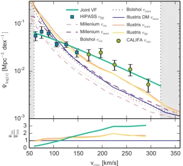
We compare our work with a number of simulations. Shown
in Figure 3 are the VFs from the Millennium (Springel
et al. 2005) and Bolshoi (Klypin et al. 2011) dark matter simulations. Here we are plotting friends-of-friends DM halos using two different halo circular velocity definitions: virial velocity vvir and maximum circular velocity vmax. In addition,
we show the Illustris-1 DM-only run vmax-based VF,
constructed for halos withMDM >1010M.
Figure 3. Zoomed-in view showing the combined CALIFA+HIPASS VF and the best Schechterfit, shown as a thick solid teal line. In the top panel, dark-matter-only halo VFs from Millenium and Bolshoi simulations are shown as purple and pink dashed and dotted lines, respectively. vmax VF from Illustris-1
dark-matter-only simulation is shown by a thin dark blue line. Full-physics Illustris-1 simulation VFs, calculated using the subhalo vmax and circular
velocity at 80% stellar mass radius(v80) are displayed as orange and yellow
solid lines, respectively. The lower panel shows the ratio between the baryonic simulated VFs, the combined CALIFA+HIPASS fit and the DM-only Illustris VF. See Section3.5for a description, discussion, and references.
Table 1
Schechter Function Fit Parameters for CALIFA+HIPASS VF (Equation (1))
*
Y [´10-3Mpc−3]
v* (km s−1) α 130.0±35.8 89.3±32.8 0.2±0.6
Table 2
CALIFA-HIPASS Velocity Function Values
Survey vcirc(km s−1) Y(log10 circv )[×10−3Mpc−3]
63.0 56.1±12.2 75.3 68.2±19.1 HIPASS 89.5 62.7±10.1 106.2 36.6±4.1 125.9 36.7±5.1 147.9 24.9±5.0 172.4 22.5±6.1 197.1 24.7±5.5 CALIFA 225.4 13.7±3.3 257.7 10.9±3.0 294.6 5.2±1.6 The Astrophysical Journal Letters,827:L36(6pp), 2016 August 20 BekeraitĖ ET AL.
We also include two VFs measured from Illustris-1 full-physics simulations (Vogelsberger et al. 2014a, 2014b). Illustris vmax is calculated for all subhalos with stellar masses
* >
M 108M, while Illustris v80 is calculated as the
gravita-tional potential-induced circular rotation velocity at the 80% stellar mass radius.
It is strikingly evident that the observed VF does not agree with the dark-matter-only simulations, even though the low-velocity end of Bolshoi and Millenium simulations displays marginal agreement with the observational data. At intermedi-ate velocities the dark-matter-only VFs sit well below both the observed data and the baryonic simulation.
However, wefind that the observed VF cannot be reconciled with the Illustris v80- and vmax-based VFs, though the
full-physics simulations produce VFs that are significantly closer to the observed VF. The lack of observed galaxies is evident for velocities lower than vcirc≈ 120 km s−1. This fact was already
shown in Gonzalez et al. (2000), Papastergis et al. (2011), Abramson et al.(2014), andZ10, however, wefind it worthy to revisit their results using the latest hydrodynamical simulation results.
Interestingly, at the intermediate velocities the predicted VFs are systematically offset from the observations, differing by up to a factor of 3. This discrepancy is not related to the “under-abundance” problem.
The mismatch between simulations and observations is either a result of an inconsistency in the way that observations and simulations are measuring the VF, or the structure of simulated galaxies is inconsistent with the structure of observed galaxies. We have not yet performed a fully fair comparison between the simulations and observations using the 80% light radius in both cases, employing adequate surface brightness cuts and including projection effects for the simulation. In a very recent paper by Macciò et al.(2016) it was shown that at least some of the tension between the data and models at the low end of the VF can be alleviated by considering the finite extent of HI disks and relatively larger vertical velocity dispersion. Observational confirmation of their result would go a long way toward explaining the tension in the VF comparison at low circular velocities. We additionally note that while the Illustris VF does not fully match the observed data at high circular velocities, further study of the effects of baryons on the masses and structure of dark matter halos may close the remaining gap. The difference between observed and simu-lated VFs should be considered to be a constraint on the future generations of galaxy formation models.
4. CONCLUSIONS
In this work we measure the CALIFA stellar VF, derived from a sample of 226 stellar velocity fields. To our best knowledge, it is the first directly measured VF that includes early-type fast rotators as well as late-types.
We then combined this VF with the HIPASS VF to obtain the first directly measured VF that simultaneously covers a wide range of circular velocities and morphological types. This has the benefit of using the space density and velocity data measured from the same surveys, without assuming scaling relations or conversions between kinematic observables. The combined VF is complete in the range of 60 <vcirc<
320 km s−1. Wefind that the Illustris simulation VF does not reproduce the observed data in both the low- and high-velocity ranges.
The differences between ΛCDM predictions and the
observed VF are not dissimilar to those found when comparing the halo and stellar mass functions. There, physical processes that are important for galaxy formation cause a decoupling of the halo and galaxy growth. By highlighting similar discre-pancies, this work opens a new window for comparison with theory that should deepen our understanding of galaxy evolution. The resulting VF is expected to provide constraints on galaxy assembly and evolution models, and insights into baryonic angular momentum, and is expected to help improve halo occupation distribution and semi-analytic disk formation models.
The authors would like to express gratitude to Louis Abramson for kindly providing VF data and for assistance with interpreting it. We sincerely thank the referee for the insightful comments.
S.B. acknowledges support from BMBF through the Erasmus-F project(grant number 05 A12BA1) and is grateful to Leibniz-Institut für Astrophysik Potsdam for its hospitality during her guest stay there in 2016. J.F.B. acknowledges support from grant AYA2013-48226-C3-1-P from the Spanish Ministry of Economy and Competitiveness(MINECO). C.J.W. acknowledges support through the Marie Curie Career Integration Grant 303912. S.F.S. thanks the CONACYT-125180 and DGAPA-IA100815 projects for providing support during this study. D.O. thanks the University of Western Australia for its support via a Research Collaboration Award. K.S. acknowledges funding from the Natural Sciences and Engineering Research Council of Canada.
This study makes use of the data provided by the Calar Alto Legacy Integral Field Area (CALIFA) survey (http://www. califa.caha.es). This work is based on observations collected at
the Centro Astronmico Hispano Alemán (CAHA) at Calar
Alto, operated jointly by the Max-Planck-Institut fr Astronomie and the Instituto de Astrofisica de Andalucia (CSIC). CALIFA is thefirst legacy survey being performed at Calar Alto.
We have extensively used the open source data analysis and visualization tools Matplotlib(Hunter2007) and SciPy (Jones et al.2001-2015).
REFERENCES
Abramson, L. E., Williams, R. J., Benson, A. J., Kollmeier, J. A., & Mulchaey, J. S. 2014,ApJ,793, 49
Bekeraitė, S., Walcher, J., & Falcón-Barroso, J. 2016, ApJ, in press Binney, J., & Tremaine, S. 2008, Galactic Dynamics(2nd ed.; Princeton, NJ:
Princeton Univ. Press)
Chae, K.-H. 2010,MNRAS,402, 2031
Croton, D. J. 2013,PASA,30, 52
Desai, V., Dalcanton, J. J., Mayer, L., et al. 2004,MNRAS,351, 265
García-Benito, R., Zibetti, S., Sánchez, S. F., et al. 2015,A&A,576, A135
Gonzalez, A. H., Williams, K. A., Bullock, J. S., Kolatt, T. S., & Primack, J. R. 2000,ApJ,528, 145
Hunter, J. D. 2007,CSE,9, 90
Husemann, B., Jahnke, K., Sánchez, S. F., et al. 2013,A&A,549, A87
Jones, E., Oliphant, T., Peterson, P., et al. 2001-2015, SciPy: Open Source Scientific Tools for Python, Online (accessed 2015 June 17)
Kalinova, V., van de Ven, G., Lyubenova, M., et al. 2016, MNRAS, submitted Klypin, A., Karachentsev, I., Makarov, D., & Nasonova, O. 2015,MNRAS,
454, 1798
Klypin, A. A., Trujillo-Gomez, S., & Primack, J. 2011,ApJ,740, 102
Kochanek, C. S., & White, M. 2001,ApJ,559, 531
Krajnović, D., Bacon, R., Cappellari, M., et al. 2008,MNRAS,390, 93
Macciò, A. V., Udrescu, S. M., Dutton, A. A., et al. 2016, arXiv:1607.01028
Meyer, M. J., Zwaan, M. A., Webster, R. L., Schneider, S., & Staveley-Smith, L. 2008,MNRAS,391, 1712
Newman, J. A., & Davis, M. 2000,ApJL,534, L11
Newman, J. A., & Davis, M. 2002,ApJ,564, 567
Obreschkow, D., Ma, X., Meyer, M., et al. 2013,ApJ,766, 137
Papastergis, E., Martin, A. M., Giovanelli, R., & Haynes, M. P. 2011,ApJ,
739, 38
Roth, M. M., Kelz, A., Fechner, T., et al. 2005,PASP,117, 620
Sánchez, S. F., Kennicutt, R. C., Gil de Paz, A., et al. 2012,A&A,538, A8
Schmidt, M. 1968,ApJ,151, 393
Scott, D. W. 1979,Biometrika, 66, 605
Springel, V., White, S. D. M., Jenkins, A., et al. 2005,Natur,435, 629
Verheijen, M. A. W., Bershady, M. A., Andersen, D. R., et al. 2004,AN,
325, 151
Vogelsberger, M., Genel, S., Springel, V., et al. 2014a,MNRAS,444, 1518
Vogelsberger, M., Genel, S., Springel, V., et al. 2014b,Natur,509, 177
Walcher, C. J., Wisotzki, L., Bekeraité, S., et al. 2014,A&A,569, A1
Zwaan, M. A., Meyer, M. J., & Staveley-Smith, L. 2010, MNRAS,
403, 1969
Zwaan, M. A., Staveley-Smith, L., Koribalski, B. S., et al. 2003,AJ,125, 2842