HAL Id: hal-00358755
https://hal.archives-ouvertes.fr/hal-00358755
Submitted on 4 Feb 2009
HAL is a multi-disciplinary open access
archive for the deposit and dissemination of
sci-entific research documents, whether they are
pub-lished or not. The documents may come from
teaching and research institutions in France or
abroad, or from public or private research centers.
L’archive ouverte pluridisciplinaire HAL, est
destinée au dépôt et à la diffusion de documents
scientifiques de niveau recherche, publiés ou non,
émanant des établissements d’enseignement et de
recherche français ou étrangers, des laboratoires
publics ou privés.
A dynamical-system analysis of the optimum s-gradient
algorithm
Luc Pronzato, Henry Wynn, Anatoly Zhigljavsky
To cite this version:
Luc Pronzato, Henry Wynn, Anatoly Zhigljavsky. A dynamical-system analysis of the optimum
s-gradient algorithm. Luc Pronzato, Anatoly Zhigljavsky. Optimal Design and Related Areas in
Op-timization and Statistics, Springer Verlag, pp.39-80, 2009, Springer OpOp-timization and its Applications,
�10.1007/978-0-387-79936-0_3�. �hal-00358755�
A dynamical-system analysis of the optimum
s-gradient algorithm
L. Pronzato, H.P. Wynn, and A. Zhigljavsky
Summary. We study the asymptotic behaviour of Forsythe’s s-optimum gradient algorithm for the minimization of a quadratic function in Rdusing a renormalization that converts the algorithm into iterations applied to a probability measure. Bounds on the performance of the algorithm (rate of convergence) are obtained through optimum design theory and the limiting behaviour of the algorithm for s = 2 is investigated into details. Algorithms that switch periodically between s = 1 and s = 2 are shown to converge much faster than when s is fixed at 2.
1.1 Introduction
The asymptotic behavior of the steepest-descent algorithm (that is, the opti-mum 1-gradient method) for the minimization of a quadratic function in Rd
is well-known, see Akaike (1959); Nocedal et al. (1998, 2002) and Chap. 7 of (Pronzato et al., 2000). Any vector y of norm one with two nonzero compo-nents only is a fixed point for two iterations of the algorithm after a suitable renormalization. The main result is that, in the renormalized space, one typ-ically observes convergence to a two-point limit set which lies in the space spanned by the eigenvectors corresponding to the smallest and largest eigen-values of the matrix A of the quadratic function. The proof for bounded quadratic operators in Hilbert space is similar to the proof for Rd although
more technical, see Pronzato et al. (2001, 2006). In both cases, the method consists of converting the renormalized algorithm into iterations applied to a measure νk supported on the spectrum of A. The additional technicalities
arise from the fact that in the Hilbert space case the measure may be contin-uous. For s = 1, the well-known inequality of Kantorovich gives a bound on the rate of convergence of the algorithm, see Kantorovich and Akilov (1982) and (Luenberger, 1973, p. 151). However, the actual asymptotic rate of con-vergence, although satisfying the Kantorovich bound, depends on the starting point and is difficult to predict; a lower bound can be obtained (Pronzato et al., 2001, 2006) from considerations on the stability of the fixed points for the attractor.
The situation is much more complicated for the optimum s-gradient algo-rithm with s ≥ 2 and the paper extends the results presented in (Forsythe,
1968) in several directions. First, two different sequences are shown to be monotonically increasing along the trajectory followed by the algorithm (af-ter a suitable renormalization) and a link with optimum design theory is established for the construction of upper bounds for these sequences. Second, the case s = 2 is investigated into details and a precise characterization of the limiting behavior of the renormalized algorithm is given. Finally, we show how switching periodically between the algorithms with respectively s = 1 and s = 2 drastically improves the rate of convergence. The resulting algorithm is shown to have superlinear convergence in R3 and we give some
explana-tions for the fast convergence observed in simulaexplana-tions in Rd with d large: by
switching periodically between algorithms one destroys the stability of the limiting behavior obtained when s is fixed (which is always associated with slow convergence).
The chapter is organized as follows. Sect. 1.2 presents the optimum s-gradient algorithm for the minimization of a quadratic function in Rd, first in
the original space and then, after a suitable renormalization, as a transforma-tion applied to a probability measure. Rates of convergence are defined in the same section. The asymptotic behavior of the optimum s-gradient algorithm in Rd is considered in Sect. 1.3 where some of the properties established in
(Forsythe, 1968) are recalled. The analysis for the case s = 2 is detailed in Sect. 1.4. Switching strategies that periodically alternate between s = 1 and s = 2 are considered in Sect. 1.5.
1.2 The optimum s-gradient algorithm for the
minimization of a quadratic function
Let A be a real bounded self-adjoint (symmetric) operator in a real Hilbert space H with inner product (x, y) and norm given by kxk = (x, x)1/2. We
shall assume that A is positive, bounded below, and its spectral boundaries will be denoted by m and M :
m = inf
kxk=1(Ax, x) , M = supkxk=1(Ax, x) ,
with 0 < m < M < ∞. The function f0 to be minimized with respect to
t ∈ H is the quadratic form f0(t) =
1
2(At, t) − (t, y)
for some y ∈ H, the minimum of which is located at t∗ = A−1y. By a
trans-lation of the origin, which corresponds to the definition of x = t − t∗ as the
variable of interest, the minimization of f0 becomes equivalent to that of f
defined by
f (x) =1
which is minimum at x∗ = 0. The directional derivative of f at x in the
direction u is
∇uf (x) = (Ax, u) .
The direction of steepest descent at x is −g, with g = g(x) = Ax the gradient of f at x. The minimum of f along the line L1(x) = {x + γAx , γ ∈ R} is
obtained for the optimum step-length
γ∗= −(Ag, g)(g, g) ,
which corresponds to the usual steepest-descent algorithm. One iteration of the steepest-descent algorithm, or optimum 1-gradient method, is thus
xk+1= xk−
(gk, gk)
(Agk, gk)
gk, (1.2)
with gk= Axkand x0some initial element in H. For any integer s ≥ 1, define
the s-dimensional plane of steepest descent by Ls(x) = {x +
s
X
i=1
γiAix , γi ∈ R for all i} .
In the optimum s-gradient method, xk+1is chosen as the point in Ls(xk) that
minimizes f . When H = Rd, A is d × d symmetric positive-definite matrix
with minimum and maximum eigenvalues respectively m and M , and xk+1is
uniquely defined provided that the d eigenvalues of A are all distinct. Also, in that case Ld(xk) = Rdand only the case s ≤ d is of interest. We shall give
special attention to the case s = 2. 1.2.1 Updating rules
Similarly to (Pronzato et al., 2001, 2006) and Chap. 2 of this volume, consider the renormalized gradient
z(x) = g(x) (g(x), g(x))1/2,
so that (z(x), z(x)) = 1 and denote zk = z(xk) for all k. Also define
µk
j = (Ajzk, zk) , j ∈ Z , (1.3)
so that µk
0 = 1 for any k and the optimum step-length of the optimum
1-gradient at step k is −1/µk
1, see (1.2). The optimum choice of the s γi’s in the
optimum s-gradient can be obtained by direct minimization of f over Ls(xk).
A simpler construction follows from the observation that gk+1, and thus zk+1,
optimum step-lengthes at step k, −→γk = (γ1k, . . . , γsk)⊤, is thus solution of the
following system of s linear equations
Mks,1−→γk= −(1, µk1, . . . , µks−1)⊤, (1.4)
where Mks,1 is the s × s (symmetric) matrix with element (i, j) given by
{Mk
s,1}i,j = µki+j−1.
The following remark will be important later on, when we shall compare the rates of convergence of different algorithms.
Remark 1. One may notice that one step of the optimum s-gradient method starting from some x in H corresponds to s successive steps of the conjugate gradient algorithm starting from the same x, see (Luenberger, 1973, p. 179). ¤ The next remark shows the connection with optimum design of experi-ments, which will be further considered in Sect. 1.2.3 (see also Pronzato et al. (2005) where the connection is developed around the case of the steepest-descent algorithm).
Remark 2. Consider Least-Squares (LS) estimation in a regression model
s
X
i=1
γiti = −1 + εi
with (εi) a sequence of i.i.d. errors with zero mean. Assume that the ti’s
are generated according to a probability (design) measure ξ. Then, the LS estimator of the parameters γi, i = 1, . . . , s is
ˆ γ = − ·Z (t, t2, . . . , ts)⊤(t, t2, . . . , ts) ξ(dt) ¸−1 Z (t, t2, . . . , ts)⊤ξ(dt)
and coincides with −→γk when ξ is such that
Z
tj+1ξ(dt) = µkj, j = 0, 1, 2 . . .
The information matrix M(ξ) for this LS estimation problem then coincides with Mk
s,1. ¤
Using (1.4), one iteration of the optimum s-gradient method thus gives xk+1= Qks(A)xk, gk+1= Qks(A)gk (1.5)
where Qk
s(t) is the polynomial Qks(t) = 1 +
Ps
i=1γiktiwith the γki solutions of
(1.4). Note that the use of any other polynomial P (t) of degree s or less, and such that P (0) = 1, yields a larger value for f (xk+1). Using (1.4), we obtain
Qks(t) = 1 − (1, µk1, . . . , µks−1) [Mks,1]−1 t .. . ts
and direct calculations give
Qks(t) = ¯ ¯ ¯ ¯ ¯ ¯ ¯ ¯ ¯ 1 µk 1 . . . µks−1 1 µk 1 µk2 . . . µks t .. . ... . . . ... ... µk s µks+1. . . µk2s−1ts ¯ ¯ ¯ ¯ ¯ ¯ ¯ ¯ ¯ |Mk s,1| (1.6) where, for any square matrix M, |M| denotes its determinant. The derivation of the updating rule for the normalized gradient zk relies on the computation
of the inner product (gk+1, gk+1). From the orthogonality property of gk+1to
gk, Agk, . . . , As−1gk we get (gk+1, gk+1) = (gk+1, γskAsgk) = γsk(Qks(A)Asgk, gk) = ¯ ¯ ¯ ¯ ¯ ¯ ¯ ¯ ¯ 1 µk 1 . . . µks−1 µks µk 1 µk2 . . . µks µks+1 .. . ... . . . ... ... µk s µks+1. . . µk2s−1 µk2s ¯ ¯ ¯ ¯ ¯ ¯ ¯ ¯ ¯ |Mk s,1| γsk(gk, gk) , (1.7) where γk
s, the coefficient of ts in Qks(t), is given by
γsk = ¯ ¯ ¯ ¯ ¯ ¯ ¯ ¯ ¯ 1 µk 1 . . . µks−1 µk 1 µk2 . . . µks .. . ... . . . ... µk s−1µks . . . µk2s−2 ¯ ¯ ¯ ¯ ¯ ¯ ¯ ¯ ¯ |Mk s,1| . (1.8)
1.2.2 The optimum s-gradient algorithm as a sequence of transformations of a probability measure
When H = Rd, we can assume that A is already diagonalized, with eigenvalues 0 < m = λ1 ≤ λ2 ≤ · · · ≤ λd = M , and consider [zk]2i, with [zk]i the i-th
component of zk, as a mass on the eigenvalue λi(note thatPdi=1[zk]2i = µk0 =
1). Define the discrete probability measure νk supported on (λ1, . . . , λd) by
νk(λi) = [zk]2i, so that its j-th moment is µkj, j ∈ Z, see (1.3).
Remark 3. When two eigenvalues λi and λj of A are equal, their masses [zk]2i
and [zk]2j can be added since the updating rule is the same for the two
the optimum s-gradient algorithm, confounding masses associated with equal eigenvalues simply amounts to reducing the dimension of H and we shall there-fore assume that all eigenvalues of A are different when studying the evolution
of νk. ¤
In the general case where H is a Hilbert space, let Eλ denote the spectral
family associated with the operator A; we then define the measure νk by
νk(dλ) = d(Eλzk, zk), m ≤ λ ≤ M. In both cases H = Rd and H a Hilbert
space, we consider νk as the spectral measure of A at the iteration k of the
algorithm, and write
µkj =
Z
tiνk(dt) .
For any measure ν on the interval [m, M ], any α ∈ R and any positive integer m define
Mm,α(ν) =
Z
tα(1, t, t2, . . . , tm)⊤(1, t, t2, . . . , tm) ν(dt) . (1.9)
For both H = Rdand H a Hilbert space, the iteration on z
kcan be written as zk → zk+1= Tz(zk) = gk+1 (gk+1, gk+1)1/2 = (gk, gk) 1/2 (gk+1, gk+1)1/2 Qks(A)zk = |M k s,1| |Mk s,0|1/2|Mks−1,0|1/2 Qks(A)zk, (1.10) with Mk
s,1 = Ms−1,1(νk) and Mkm,0 = Mm,0(νk), i.e. the (m + 1) × (m + 1)
matrix with element (i, j) given by {Mk
m,0}i,j= µki+j−2. The iteration on zk
can be interpreted as a transformation of the measure νk
νk→ νk+1= Tν(νk) with νk+1(dx) = Hk(x)νk(dx) , (1.11)
where, using (1.5, 1.6, 1.7) and (1.8), we have Hk(x) = [Qks(x)]2|Mks,1|2 |Mk s,0||Mks−1,0| (1.12) = (1, x, . . . , xs)[Mk s,0]−1 1 x .. . xs − (1, x, . . . , xs−1)[Mk s−1,0]−1 1 x .. . xs−1 . As moment matrices, Mk
s,1 and Mkm,0 are positive semi-definite and
|Mk
s,1| ≥ 0 for any s ≥ 1 (respectively |Mkm,0| ≥ 0 for any m ≥ 0), with
on m points or less). Also note that from the construction of the polynomial Qk
s(t), see (1.5), we have
Z
Qks(t) tiνk(dt) = (Qsk(A)gk, Aigk) = 0 , i = 0, . . . , s − 1 , (1.13)
which can be interpreted as an orthogonality property between the polyno-mials Qk
s(t) and ti for i = 0, . . . , s − 1. From this we can easily deduce the
following.
Theorem 1.Assume that νk is supported on s + 1 points at least. Then the
polynomial Qks(t) defined by (1.5) has s roots in the open interval (m, M ).
Proof. Let ζi, i = 1, . . . , q − 1, denote the roots of Qks(t) in (m, M ). Suppose
that q − 1 < s. Consider the polynomial T (t) = (−1)q−1Qk s(m)
Qq−1
i=1(t −
ζi), it satisfies T (t)Qks(t) > 0 for all t ∈ (m, M), t 6= ζi. Therefore,
R T (t)Qk
s(t)νk(dt) > 0, which contradicts (1.13) since T (t) has degree q − 1 ≤
s − 1.
Remark 4. Theorem 1 implies that Qk
s(m) has the same sign as Qks(0) =
(−1)s|Mk
s−1,0|/|Mks,1|, that is, (−1)s. Similarly, Qks(M ) has the same sign
as limt→∞Qks(t) which is positive. ¤
Using the orthogonality property (1.13), we can also prove the next two theorems concerning the support of νk, see Forsythe (1968).
Theorem 2.Assume that the measure νk is supported on s+1 points at least.
Then this is also true for the measure νk+1 obtained through (1.11).
Proof. We only need to consider the case when the support Sk of νk is finite,
that is, when H = Rd. Suppose that ν
kis supported on n points, n ≥ s+1. The
determinants |Mk
s,1|, |Mks,0| and |Mks−1,1| in (1.12) are thus strictly positive.
Let q be the largest integer such that there exist λi1 < λi2 < · · · < λiq in Sk
with Qk s(λij)Q
k
s(λij+1) < 0, j = 1, . . . , q − 1. We shall prove that q ≥ s + 1.
From (1.11, 1.12) it implies that νk is supported on s + 1 points at least.
From (1.13),R Qk
s(t) νk(dt) = 0, so that there exist λi1 and λi2 in Sk with
Qk s(λi1)Q
k
s(λi2) < 0, therefore q ≥ 2. Suppose that q ≤ s. By construction
Qk
s(λi1) is of the same sign as Q
k
s(m) and we can construct q disjoint open
intervals Λj, j = 1, . . . , q such that λij ∈ Λj and Q
k
s(λi)Qks(λij) ≥ 0 for all
λi∈ Sk∩ Λj with ∪qj=1Λ¯j= [m, M ], where ¯Λjis the closure of Λj (notice that
Qk
s(λ) may change sign in Λjbut all the Qks(λi)’s are of the same sign for λi∈
Sk∩Λj). Consider the q−1 scalars ζi, i = 1, . . . , q−1, defined by the endpoints
of the Λj’s, m and M excluded; they satisfy λi1< ζ1< λi2 < · · · < ζq−1< λiq.
Form now the polynomial T (t) = (−1)s+q−1(t − ζ
1) × · · · × (t − ζq−1), one
can check that Qk
s(λi)T (λi) ≥ 0 for all λi in Sk. Also, Qks(λij)T (λij) > 0
for j = 1, . . . , q. This implies Pd
i=1T (λi)Qks(λi)[zk]2i > 0, which contradicts
Corollary 1.If x0 is such that ν0 is supported on n0= s + 1 points at least,
then (gk, gk) > 0 for all k ≥ 1. Also, the determinants of all (m + 1) × (m + 1)
moment matrices Mm,α(νk), see (1.9), are strictly positive for all k ≥ 1.
Theorem 3.Assume that ν0is supported on n0= s+1 points. Then ν2k= ν0
for all k.
Proof. It is enough to prove that g2k is parallel to g0, and thus that g2 is
parallel to g0. Since the updating rule only concerns nonzero components,
we may assume that d = s + 1. We have g1 = Q0s(A)g0, g2 = Q1s(A)g1, g1 is
orthogonal to g0, Ag0, . . . , As−1g0, which are independent, and g2is orthogonal
to g1. We can thus decompose g2with respect to the basis g0, Ag0, . . . , As−1g0
as g2= s−1 X i=0 αiAig0.
Now, g2 is orthogonal to Ag1, and thus
g⊤1Ag2= 0 = s−1 X i=0 αig1⊤Ai+1g0= αs−1g⊤1Asg0 with g⊤
1Asg0 6= 0 since otherwise g1 would be zero. Therefore, αs−1 = 0.
Similarly, g2is orthogonal to A2g1, which gives
0 =
s−2
X
i=0
αig⊤1Ai+2g0= αs−2g1⊤Asg0
so that αs−2= 0. Continuing like that up to g1⊤As−1g2we obtain α1= α2=
· · · = αs−1 = 0 and g2 = α0g0. Notice that α0 > 0 since (A−1g2, g0) =
(A−1g
1, g1), see (1.18).
The transformation zk → zk+1 = Tz(zk) (respectively νk → νk+1 =
Tν(νk)) can be considered as defining a dynamical system with state zk ∈ H
at iteration k (respectively, νk ∈ Π, the set of probability measures defined
on the spectrum of A). One purpose of the paper is to investigate the limit set of the orbit of the system starting at z0or ν0. As it is classical in the study of
stability of dynamical systems where Lyapunov functions often play a key role (through the Lyapunov Stability Theorem or Lasalle’s Invariance Principle, see, e.g., (Elaydi, 2005, Chap. 4)), the presence of monotone sequences in the dynamics of the renormalized algorithm will be an important ingredient of the analysis. Theorem 3 shows that the behavior of the renormalized algo-rithm may be periodic with period 2. We shall see that this type of behavior is typical, although the structure of the attractor may be rather complicated.
1.2.3 Rates of convergence and monotone sequences Rates of convergence
Consider the following rate of convergence of the algorithm at iteration k, rk = f (xk+1) f (xk) = (Axk+1, xk+1) (Axk, xk) = (A −1g k+1, gk+1) (A−1g k, gk) . (1.14) From the orthogonality property of gk+1we have
(A−1gk+1, gk+1) = (A−1Qks(A)gk, gk+1) = (A−1gk, gk+1)
and thus, using (1.6),
rk = |M k s,−1| |Mk s,1| µk−1 with Mk
s,−1 = Ms,−1(νk), see (1.9), that is, the (s+1)×(s+1) moment matrix
with element (i, j) given by {Mk
s,−1}i,j = µki+j−3. Using the orthogonality
property of gk+1 again, we can easily prove that the sequence of rates (rk) is
non-decreasing along the trajectory followed by the algorithm.
Theorem 4.When x0 is such that ν0 is supported on s + 1 points at least,
the rate of convergence rk defined by (1.14) is non-decreasing along the path
followed by the optimum s-gradient algorithm. It also satisfies rk≤ R∗s= Ts−2
µ ̺ + 1 ̺ − 1
(1.15) where ̺ = M/m is the condition number of A and Ts(t) is the s-th Chebyshev
polynomial (normalized so that maxt∈[−1,1]|Ts(t)| = 1)
Ts(t) = cos[s arccos(t)] =
(t +√t2− 1)s+ (t −√t2− 1)s
2 . (1.16)
Moreover, the equality in (1.15) is obtained when νk is the measure νs∗defined
by ν∗
s(y0) = νs∗(ys) = 1/(2s) , νs∗(yj) = 1/s , 1 ≤ j ≤ s − 1 , (1.17)
where yj= (M + m)/2 + [cos(jπ/s)](M − m)/2.
Proof. From Corollary 1, (g0, g0) > 0 implies (gk, gk) > 0 for all k and rk is
thus well defined. Straightforward manipulations give (A−1g
k+1, gk+1) − (A−1gk+2, gk) =¡A−1[Qks(A) − Qk+1s (A)]gk, Qks(A)gk¢
= Ã A−1 s X i=1 (γik− γik+1)Aigk, Qks(A)gk ! = 0 (1.18)
where equality to zero follows from (1.13). Therefore, from the Cauchy– Schwarz inequality,
(A−1gk+1, gk+1)2= (A−1gk+2, gk)2≤ (A−1gk+2, gk+2)(A−1gk, gk)
and rk≤ rk+1, with equality if and only if gk+2= αgkfor some α ∈ R+(α > 0
since (A−1gk+2, gk) = (A−1gk+1, gk+1)). This shows that rkis non-decreasing.
The rate (1.14) can also be written as
rk =£µk−1{(Mks,−1)−1}1,1¤ −1
.
Define the measure ¯νk by ¯νk(dt) = νk(dt)/(tµk−1) (so thatR ¯νk(dt) = 1) and
denote ¯Mkm,nthe matrix obtained by substituting ¯νk for νk in Mkm,nfor any
n, m. Then, ¯Mks,0= Mk
s,−1/µk−1 and rk =£{( ¯Mks,0)−1}1,1¤ −1
. The maximum value for rk is thus obtained for the Ds-optimal measure ¯νs∗ on [m, M ] for
the estimation θ0 in the linear regression model η(θ, x) = Psi=0θixi with
i.i.d. errors, see, e.g., (Fedorov, 1972, p. 144) and (Silvey, 1980, p. 10) (¯ν∗ s is
also c-optimal for c = (1, 0, . . . , 0)⊤). This measure is uniquely defined, see
Hoel and Levine (1964), (Sahm, 1998, p. 52): it is supported at the s + 1 points yj = (M + m)/2 + [cos(jπ/s)](M − m)/2, j = 0, . . . , s, and each yj
receives a weight proportional to αj/yj, with α0= αs = 1/2 and αj = 1 for
j = 1, . . . , s − 1. Applying the transformation ν(dt) = t¯ν(dt)µ−1 we obtain
the measure ν∗
s given by (1.17).
Remark 5. Meinardus (1963) and Forsythe (1968) arrive at the result (1.15) by a different route. They write
rk= (A−1g k+1, gk+1) (A−1g k, gk) =R [Q k s(t)]2t−1νk(dt) µk −1 . Since Qk
s(t) minimizes f (xk+1), rk ≤ (1/µk−1)R P2(t) t−1νk(dt) for any
s-degree polynomial P (t) such that P (0) = 1. Equivalently, rk≤ R S
2(t) t−1ν k(dt)
S2(0)µk −1
for any s-degree polynomial S(t). Take S(t) = S∗(t) = T
s[(M + m − 2t)/(M −
m)], so that S2(t) ≤ 1 for t ∈ [m, M], then r
k satisfies rk ≤ [S∗(0)]−2 = R∗s
with R∗
sgiven by (1.15). ¤
Notice that Ts[(̺ + 1)/(̺ − 1)] > 1 in (1.15), so that we have the following.
Corollary 2.If x0 is such that ν0 is supported on s + 1 points at least, then
the optimum s-gradient algorithm converges linearly to the optimum, that is, 0 < c1=f (x1) f (x0) ≤ f (xk+1) f (xk) ≤ R ∗ s< 1 , for all k .
Moreover, the convergence slows down monotonically on the route to the op-timum and the rate rk given by (1.14) tends to a limit r∞.
The monotonicity of the sequence (rk), together with Theorem 3, has the
following consequence.
Corollary 3.Assume that ν0is supported on n0= s + 1 points. Then rk+1=
rk for all k.
Other rates of convergence can be defined as Rk(W ) =
(W gk+1, gk+1)
(W gk, gk)
(1.19) with W be a bounded positive self-adjoint operator in H. However, the fol-lowing theorem shows that all such rates are asymptotically equivalent, see Pronzato et al. (2006).
Theorem 5.Let W be a bounded positive self-adjoint operator in H, with bounds c and C such that 0 < c < C < ∞ (when H = Rd, W is a d × d
positive-definite matrix with minimum and maximum eigenvalues respectively c and C). Consider the rate of convergence defined by (1.19) if kgkk 6= 0
and Rk(W ) = 1 otherwise. Apply the optimum s-gradient algorithm (1.5),
initialized at g0 = g(x0), for the minimization of f (x) given by (1.1). Then
the limit R(W, x0) = lim n→∞ "n−1 Y k=0 Rk(W ) #1/n
exists for all x0 in H and R(W, x0) = R(x0) does not depend on W . In
particular, R(W, x0) = r∞= lim n→∞ Ãn−1 Y k=0 rk !1/n (1.20) with rk defined by (1.14).
Proof. Assume that x0 is such that for some k ≥ 0, kgk+1k = 0 with kgik > 0
for all i ≤ k (that is, xk+1 = x∗ and xi 6= x∗ for i ≤ k). This implies
Rk(W ) = 0 for any W , and therefore R(W, x0) = R(x0) = 0.
Assume now that kgkk > 0 for all k. Consider
Vn= "n−1 Y k=0 Rk(W ) #1/n = "n−1 Y k=0 (W gk+1, gk+1) (W gk, gk) #1/n =· (W gn, gn) (W g0, g0) ¸1/n . We have, ∀z ∈ H , ckzk2≤ (W z, z) ≤ Ckzk2, and thus (c/C)1/n· (gn, gn) (g0, g0) ¸1/n ≤ Vn≤ (C/c)1/n · (gn, gn) (g0, g0) ¸1/n .
Since (c/C)1/n → 1 and (C/c)1/n → 1 as n → ∞, lim inf
n→∞Vn and
lim supn→∞ Vn do not depend on W . Taking W = A−1 we get Rk(W ) = rk.
The sequence (rk) is not decreasing, and thus limn→∞Vn= r∞for any W .
For any fixed ̺ = M/m, the bound R∗
s given by (1.15) tends to zero as s
tends to infinity whatever the dimension d when H = Rd, and also when H is
a Hilbert space. However, since one step of the optimum s-gradient method corresponds to s successive steps of the conjugate gradient algorithm, see Remark 1, a normalized version of the convergence rate allowing comparison with classical steepest descent is rk1/s, which is bounded by
Ns∗= (R∗s)1/s= Ts−2/s
µ ̺ + 1 ̺ − 1
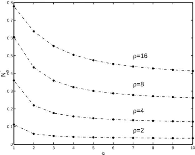
(1.21) where Ts(t) is the s-th Chebyshev polynomial, see (1.16). The quantity Ns∗is
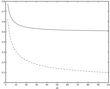
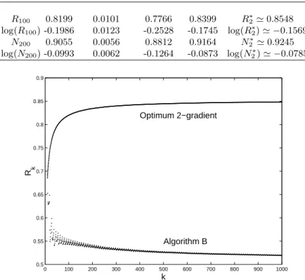
a decreasing function of s, see Fig. 1.1, but has a positive limit when s tends to infinity, lim s→∞N ∗ s = N∞∗ = (√̺− 1)2 (√̺ + 1)2. (1.22)
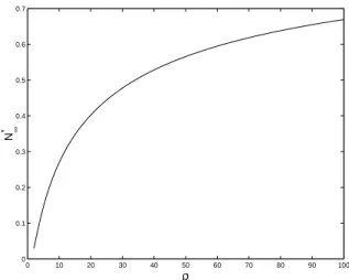
Fig. 1.2 shows the evolution of N∗
∞ as a function of the condition number ̺.
1 2 3 4 5 6 7 8 9 10 0 0.1 0.2 0.3 0.4 0.5 0.6 0.7 0.8 s Ns * ρ=16 ρ=8 ρ=4 ρ=2
Fig. 1.1.Upper bounds N∗
s, see (1.21), as functions of s for different values of the condition number ̺
A second monotone bounded sequence
Another quantity qk also turns out to be non-decreasing along the trajectory
0 10 20 30 40 50 60 70 80 90 100 0 0.1 0.2 0.3 0.4 0.5 0.6 0.7 ρ N∞ *
Fig. 1.2.Limiting value N∗
∞as a function of ̺
Theorem 6.When x0 is such that ν0 is supported on s + 1 points at least,
the quantity qk defined by
qk= (gk+1, gk+1) (γk s)2(gk, gk) , (1.23) with γk
s given by (1.8), is non-decreasing along the path followed by the
opti-mum s-gradient algorithm. Moreover, it satisfies qk ≤ qs∗=(M − m)
2s
24s−2 , for all k , (1.24)
where the equality is obtained when νk is the measure (1.17) of Theorem 4.
Proof. From Corollary 1, (g0, g0) > 0 implies (gk, gk) > 0 and γks > 0 for all
k so that qk is well defined. Using the same approach as for rk in Theorem 4,
we write (gk+1, gk+1)/γsk− (gk+2, gk)/γsk+1=¡Qks(A)gk, gk+1¢ /γsk −¡Qk+1 s (A)gk, gk+1¢ /γsk+1 =¡[Qk s(A)/γks− Qk+1s (A)/γsk+1]gk, gk+1 ¢ = Ã" (1/γsk− 1/γsk+1)I + s−1 X i=1 (γik/γsk− γik+1/γ k+1 s )Ai # gk, gk+1 ! = 0 ,
where equality to zero follows from (1.13). The Cauchy–Schwarz inequality then implies
(gk+1, gk+1)2/(γsk)2= (gk+2, gk)2/(γk+1s )2≤ (gk+2, gk+2)(gk, gk)/(γsk+1)2
and qk≤ qk+1with equality if and only if gk+2= αgkfor some α ∈ R+(α > 0
since (gk+2, gk) = (gk+1, gk+1)γsk+1/γsk and γsk> 0 for all k, see Corollary 1).
This shows that qk is non-decreasing.
The determination of the probability measure that maximizes qk is again
related to optimal design theory. Using (1.7) and (1.8), we obtain qk= |Mk s,0| |Mk s−1,0| .
Hence, using the inversion of a partitioned matrix, we can write
qk= µk2s− (1, µk1, . . . , µks−1)(Mks−1,0)−1 1 µk 1 .. . µk s−1 =³©(Mk s,0)−1 ª s+1,s+1 ´−1 ,
so that the maximization of qk with respect to νk is equivalent to the
de-termination of a Ds-optimum measure on [m, M ] for the estimation of θs in
the linear regression model η(θ, x) = Ps
i=0θixi with i.i.d. errors (or to the
determination of a c-optimal measure on [m, M ] with c = (0, . . . , 0, 1)⊤). This
measure is uniquely defined, see (Kiefer and Wolfowitz, 1959, p. 283): when the design interval is normalized to [−1, 1], the optimum measure ξ∗ is
sup-ported on s + 1 points given by ±1 and the s − 1 zeros of the derivative of s-th Chebyshev polynomial Ts(t) given by (1.16) and the weights are
ξ∗(−1) = ξ∗(1) = 1/(2s) , ξ∗(cos[jπ/s]) = 1/s , 1 ≤ j ≤ s − 1 . The transformation t ∈ [−1, 1] 7→ z = (M + m)/2 + t(M − m)/2 ∈ [m, M] gives the measure ν∗
s on [m, M ]. The associated maximum value for qk is q∗s
given by (1.24), see (Kiefer and Wolfowitz, 1959, p. 283).
The monotonicity of the sequence (qk), together with Theorem 3, implies
the following analogue to Corollary 3.
Corollary 4.Assume that ν0is supported on n0= s + 1 points. Then qk+1=
qk for all k.
As a non-decreasing and bounded sequence, (qk) tends to a limit q∞. The
existence of limiting values r∞and q∞will be essential for studying the limit
points of the orbits (z2k) or (ν2k) in the next sections. In the rest of the paper
we only consider the case where H = Rd and assume that A is diagonalized
1.3 Asymptotic behavior of the optimum s-gradient
algorithm in R
dThe situation is much more complex when s ≥ 2 than for s = 1, and we shall recall some of the properties established in (Forsythe, 1968) for H = Rd. If
x0 is such that the initial measure ν0 is supported on s points or less, the
algorithm terminates in one step. In the rest of the section we thus suppose that ν0 is supported on n0 ≥ s + 1 points. The algorithm then converges
linearly to the optimum, see Corollary 2. The set Z(x0) of limit points of the
sequence of renormalized gradients z2k satisfies the following.
Theorem 7.If x0 is such that ν0 has s + 1 support points at least, the
set Z(x0) of limit points of the sequence of renormalized gradients z2k,
k = 0, 1, 2, . . . is a closed connected subset of the d-dimensional unit sphere Sd. Any y in Z(x0) satisfies Tz2(y) = y, where Tz2(y) = Tz[Tz(y)] with Tz
defined by (1.10).
Proof. Using (1.18) we get rk+1− rk= (A−1g k+2, gk+2) (A−1g k+1, gk+1)× · 1 − (A −1g k+2, gk)2 (A−1g k+2, gk+2)(A−1gk, gk) ¸ = rk+1× · 1 − (A −1z k+2, zk)2 (A−1z k+2, zk+2)(A−1zk, zk) ¸ .
Since rk is non-decreasing and bounded, see Theorem 4, rk tends to a limit
r∞(x0) and, using Cauchy–Schwarz inequality kzk+2−zkk → 0. The set Z(x0)
of limit points of the sequence z2k is thus a continuum on Sd.
Take any y ∈ Z(x0). There exists a subsequence (ki) such that z2ki → y as
i → ∞, and z2ki+2= T
2
z(z2ki) → y since kz2ki+2− z2kik → 0. The continuity
of Tz then implies z2ki+2→ T
2
z(y) and thus Tz2(y) = y.
Obviously, the sequence (z2k+1) satisfies a similar property (consider ν1as
a new initial measure ν0), so that we only need to consider the sequence of
even iterates.
Remark 6. Forsythe (1968) conjectures that the continuum for Z(x0) is in fact
always a single point. Although it is confirmed by numerical simulations, we are not aware of any proof of attraction to a single point. One may however think of Z(x0) as the set of possible limit points for the sequence (z2k), leaving
open the possibility for attraction to a particular point y∗in Z(x
0). Examples
of sets Z(x0) will be presented in Sect. 1.4. Note that we shall speak of
at-traction and attractors although the terms are somewhat inaccurate: starting from x′
0 such that z0′ = g(x′0)/kg(x′0)k is arbitrarily close to some y in Z(x0)
yields a limit set Z(x′
0) for the iterates z2k′ close to Z(x0) but Z(x′0) 6= Z(x0).
Some coordinates [y]iof a given y in Z(x0) may equal zero, i ∈ {1, . . . , d}.
Define the asymptotic spectrum S(x0, y) at y ∈ Z(x0) as the set of eigenvalues
λisuch that [y]i6= 0 and let n = n(x0, y) be the number of points in S(x0, y).
We shall then say that S(x0, y) is a n-point asymptotic spectrum. We know
from Theorem 3 that if ν0 is supported on exactly n0 = s + 1 points then
n(x0, y) = s + 1 (and ν2k = ν0 for all k so that Z(x0) is the singleton {z0}).
In the more general situation where ν0 is supported on n0 ≥ s + 1 points,
n(x0, y) satisfies the following, see Forsythe (1968).
Theorem 8.Assume that ν0 is supported on n0 > s + 1 points. Then the
number of points n(x0, y) in the asymptotic spectrum S(x0, y) of any y ∈
Z(x0) satisfies
s + 1 ≤ n(x0, y) ≤ 2s .
Proof. Take any y in Z(x0), let n be the number of its nonzero components.
To this y we associate a measure ν through ν(λi) = [y]2i, i = 1, . . . , d and we
construct a polynomial Qs(t) from the moments of ν, see (1.6). Applying the
transformation (1.11) to ν we get the measure ν′ from which we construct
the polynomial Q′
s(t). The invariance property Tz2(y) = Tz[Tz(y)] = y, with
Tzdefined by (1.10), implies Qs(λi)Q′s(λi)[y]i= c[y]i, c > 0, where [y]iis any
nonzero component of y, i = 1, . . . , n. The equation Qs(t)Q′s(t) = c > 0 can
have between 1 and 2s solutions in (m, M ). We know already from Theorem 2 that n(x0, y) ≥ s + 1.
The following Theorem shows that when m and M are support points of ν0, then the asymptotic spectrum of any y ∈ Z(x0) also contains m and M .
Theorem 9.Assume that ν0 is supported on n0 ≥ s + 1 points and that
ν0(m) > 0, ν0(M ) > 0. Then lim infk→∞νk(m) > 0 and lim infk→∞νk(M ) >
0.
Proof. We only consider the case for M , the proof being similar for m. First notice that from Theorem 1, all roots of the polynomials Qk
s(t) lie in
the open interval (m, M ), so that νk(M ) > 0 for any k.
Suppose that lim infk→∞νk(M ) = 0. Then there exists a subsequence (ki)
such that z2ki tends to some y in Z(x0) and limi→∞ν2ki(M ) = 0. To this y we
associate a measure ν as in the proof of Theorem 8 and construct a polynomial Qs(t) from the moments of ν, see (1.6). Since ν2ki(M ) → 0, ν(M) = 0. Let
λj be the largest eigenvalue of A such that ν(λj) > 0. Then, all zeros of Qs(t)
lie in (m, λj) and the same is true for the polynomial Q′s(t) constructed from
the measure ν′ = T
ν(ν) obtained by the transformation (1.11). Hence, Qs(t)
and Q′s(t) are increasing (and positive, see Remark 4) for t between λj and
M , so that Qs(M )Q′s(M ) > Qs(λj)Q′s(λj). This implies by continuity
Q2ki
s (M )Q2ks i+1(M ) ≥ c Q2ks i(λj)Q2ks i+1(λj)
[g2ki+2] 2 d [g2ki] 2 d ≥ c2[g2ki+2] 2 j [g2ki] 2 j , i > i0,
see (1.6), and thus
[z2ki+2] 2 d [z2ki+2] 2 j ≥ c2[z2ki] 2 d [z2ki] 2 j , i > i0.
Since [zk]2d > 0 for all k and [z2ki]
2
j → ν(λj) > 0 this implies [z2ki]
2
d → ∞ as
i → ∞, which is impossible. Therefore, lim infk→∞νk(M ) > 0.
The properties above explain the asymptotic behavior of the steepest-descent algorithm in Rd: when s = 1 and ν
0 is supported on two points at
least, including m and M , then n(x0, y) = 2 for any y in Z(x0) and m and
M are in the asymptotic spectrum S(x0, y) of any y ∈ Z(x0). Therefore,
S(x0, y) = {m, M} for all y ∈ Z(x0). Since Z(x0) is a part of the unit sphere
Sd, kyk = 1 and there is only one degree of freedom. The limiting value r∞of
rk then defines the attractor uniquely and Z(x0) is a singleton.
In the case where s is even, Forsythe (1968) gives examples of invariant measures ν0 satisfying νk+2 = νk and supported on 2q points with s + 1 <
2q ≤ 2s, or supported on 2q + 1 points with s + 1 ≤ 2q + 1 < 2s. The nature of the sets Z(x0) and S(x0, y) is investigated more deeply in the next section
for the case s = 2.
1.4 The optimum 2-gradient algorithm in R
dIn all the section we omit the index k in the moments µk
j and matrices Mkm,n. The polynomial Qk 2(t) defined by (1.6) is then Qk2(t) = ¯ ¯ ¯ ¯ ¯ ¯ 1 µ1 1 µ1µ2 t µ2µ3t2 ¯ ¯ ¯ ¯ ¯ ¯ |M2,1| = ¯ ¯ ¯ ¯ ¯ ¯ 1 µ1 1 µ1µ2 t µ2µ3 t2 ¯ ¯ ¯ ¯ ¯ ¯ ¯ ¯ ¯ ¯ µ1µ2 µ2µ3 ¯ ¯ ¯ ¯ and the function Hk(x), see (1.12), is given by
Hk(x) = ¯ ¯ ¯ ¯ ¯ ¯ 1 µ1 1 µ1µ2 x µ2µ3x2 ¯ ¯ ¯ ¯ ¯ ¯ 2 ¯ ¯ ¯ ¯ 1 µ1 µ1µ2 ¯ ¯ ¯ ¯ ¯ ¯ ¯ ¯ ¯ ¯ 1 µ1µ2 µ1µ2µ3 µ2µ3µ4 ¯ ¯ ¯ ¯ ¯ ¯ (1.25) =¡ 1 x x2¢ 1 µ1µ2 µ1 µ2µ3 µ2 µ3µ4 −1 1 x x2 −¡ 1 x ¢ µ 1 µ1 µ1µ2 ¶−1 µ 1 x ¶ .
The monotone sequences (rk) and (qk) of Sect. 1.2.3, see (1.14, 1.23), are given by rk = ¯ ¯ ¯ ¯ ¯ ¯ µ−1 1 µ1 1 µ1µ2 µ1 µ2µ3 ¯ ¯ ¯ ¯ ¯ ¯ µ−1 ¯ ¯ ¯ ¯ µ1µ2 µ2µ3 ¯ ¯ ¯ ¯ , qk= ¯ ¯ ¯ ¯ ¯ ¯ 1 µ1µ2 µ1µ2µ3 µ2µ3µ4 ¯ ¯ ¯ ¯ ¯ ¯ ¯ ¯ ¯ ¯ 1 µ1 µ1µ2 ¯ ¯ ¯ ¯ . (1.26)
When ν0is supported on three points, νk+2= ν0 for all k from Theorem 3
and, when ν0is supported on less than three points, the algorithm converges
in one iteration. In the rest of the section we thus assume that ν0is supported
on more than three points. Without any loss of generality, we may take d as the number of components in the support of ν0 and m and M respectively as
the minimum and maximum values of these components. 1.4.1 A characterization of limit points through the transformation νk → νk+1
From Theorem 8, the number of components n(x0, y) of the asymptotic
spec-trum S(x0, y) of any y ∈ Z(x0) satisfies 3 ≤ n(x0, y) ≤ 4 and, from Theorem 9,
S(x0, y) always contains m and M .
Consider the function
¯ Qk2(t) = Qk 2(t)|M2,1| |M1,0|1/2|M2,0|1/2 = ¯ ¯ ¯ ¯ ¯ ¯ 1 µ1 1 µ1µ2 t µ2µ3t2 ¯ ¯ ¯ ¯ ¯ ¯ ¯ ¯ ¯ ¯ 1 µ1 µ1µ2 ¯ ¯ ¯ ¯ 1/2 ¯¯ ¯ ¯ ¯ ¯ 1 µ1µ2 µ1µ2µ3 µ2µ3µ4 ¯ ¯ ¯ ¯ ¯ ¯ 1/2. (1.27) It satisfies [ ¯Qk
2(t)]2 = Hk(t), zk+1 = ¯Qk2(A)zk, see (1.10), and can be
considered as a normalized version of Qk
2(t); zk+2 = zk is equivalent to
¯
Qk+12 (A) ¯Qk2(A)zk = zk, that is ¯Qk2(λi) ¯Qk+12 (λi) = 1 for all i’s such that
[zk]i 6= 0. ¯Qk2(t) and ¯Qk+12 (t) are second order polynomials in t with two
zeros in (m, M ), see Theorem 1, and we write ¯
Qk
2(t) = αkt2+ βkt + ωk, Q¯k+12 (t) = αk+1t2+ βk+1t + ωk+1.
From the expressions (1.26, 1.27), αk= 1/√qk for any k, so that both αk and
αk+1tend to some limit 1/√q∞, see Theorem 6. From (1.27) and (1.7, 1.8),
ωk2= (gk, gk) (gk+1, gk+1), ω 2 k+1= (gk+1, gk+1) (gk+2, gk+2).
Since kz2k+2− z2kk tends to zero, see Theorem 7, Theorem 5 implies that
Three-point asymptotic spectra
Assume that x0is such that ν0 has more than three support points. To any y
in Z(x0) we associate the measure ν defined by ν(λi) = [y]2i, i = 1, . . . , d and
denote Q2(t) the polynomial obtained through (1.6) from the moments of ν.
Denote ν′ the iterate of ν through Tν; to ν′ we associate Q′2(t) and write
Q2(t) = αt2+ βt + ω , Q′2(t) = α′t2+ β′t + ω′, (1.28)
where the coefficients satisfy α = α′= 1/√q
∞and ωω′= 1/r∞.
Suppose that n(x0, y) = 3, with S(x0, y) = {m, λj, M }, where λj is some
eigenvalue of A in (m, M ). We thus have
Q2(m)Q′2(m) = Q2(λj)Q′2(λj) = Q2(M )Q′2(M ) = 1 ,
so that Q2(t) and Q′2(t) are uniquely defined, in the sense that the number of
solutions in (β, β′, ω) is finite. (ω is a root of a 6-th degree polynomial equation,
with one value for β and β′ associated with each root. There is always one
solution at least: any measure supported on m, λj, M is invariant, so that at
least two roots exist for ω. The numerical solution of a series of examples shows that only two roots exist, which renders the product Q2(t)Q′2(t) unique, due
to the possible permutation between (β, ω) and (β′, ω′).) Fig. 1.3 presents a plot of the function Q2(t)Q′2(t) when ν gives respectively the weights 1/4, 1/4
and 1/2 to the points m = 1, λj = 4/3 and M = 2 (which gives Q2(t)Q′2(t) =
(81t2− 249t + 176)(12t2− 33t + 22)/8). 1 1.1 1.2 1.3 1.4 1.5 1.6 1.7 1.8 1.9 2 −2 −1.5 −1 −0.5 0 0.5 1 1.5 t Q 2 (t)Q ′ 2 (t) Fig. 1.3.Q2(t)Q ′ 2(t) when ν(1) = 1/4, ν(4/3) = 1/4 and ν(2) = 1/2
The orthogonality property (1.13) for i = 0 givesR Q2(t) ν(dt) = 0, that
is,
αµ2+ βµ1+ ω = 0 (1.29)
where µi = p1mi+ p2λij+ (1 − p1− p2)Mi, i = 1, 2 . . . with p1 = [y]21 and
p2= [y]2j. Since ν has three support points, its moments can be expressed as
linear combinations of µ1and µ2 through the equations
Z
ti(t − m)(t − λj)(t − M) ν(dt) = 0 , i ∈ Z .
Using (1.27) and (1.29) µ1and µ2can thus be determined from two coefficients
of Q2(t) only. After calculation, the Jacobians J1, J2 of the transformations
(µ1, µ2) → (α, β) and (µ1, µ2) → (α, ω) are found to be equal to
J1= M m + mλj+ λjM − 2µ1(m + λj+ M ) + µ 2 1+ 2µ2 2|M2,0||M1,0| , J2= µ2 1(m + λj+ M ) − 2µ1µ2− mλjM 2|M2,0||M1,0| .
The only measure ˜ν supported on {m, λj, M } for which J1 = J2 = 0 is
given by µ1 = λj, µ2 = [λj(m + λj+ M ) − mM]/2, or equivalently ˜ν(m) =
(M − λj)/[2(M − m)], ˜ν(λj) = 1/2. The solution for µ1, µ2 (and thus for ν
supported at m, λj, M ) associated with a given polynomial Q2(t) through the
pair r∞, q∞ is thus locally unique and there is no continuum for three-point
asymptotic spectra, Z(x0) is a singleton. As Fig. 1.3 illustrates, the existence
of a continuum would require the presence of an eigenvalue λ∗in the spectrum
of A to which some weight could be transferred from ν. This is only possible if Q2(λ∗)Q′2(λ∗) = 1, so that λ∗is uniquely defined (λ∗= 161/108 in Fig. 1.3).
When this happens, it corresponds to a four-point asymptotic spectrum, a situation considered next.
Four-point asymptotic spectra
We consider the same setup as above with now n(x0, y) = 4 and S(x0, y) =
{m, λj, λk, M }, where λj < λk are two eigenvalues of A in (m, M ). We thus
have
Q2(m)Q′2(m) = Q2(λj)Q′2(λj) = Q2(λk)Q′2(λk) = Q2(M )Q′2(M ) = 1 ,
where Q2(t), Q′2(t) are given by (1.28) and satisfy α = α′ = 1/√q∞, ωω′ =
1/r∞. The system of equations in (α, β, ω, α′, β′, ω′) is over-determined, which
implies the existence of a relation between r∞ and q∞. As it is the case
for three-point asymptotic spectra, to a given value for q∞ corresponds a
unique polynomial Q2(t) (up to the permutation with Q′2(t)). The measures ν
which can be obtained from the values of α, β, ω once µ4 has been expressed
as a function of µ1, µ2 and µ3using
Z
(t − m)(t − λj)(t − λk)(t − M) ν(dt) = 0 .
Consider the Jacobian J of the transformation (µ1, µ2, µ3) → (α, β, ω).
Set-ting J to zero defines a two-dimensional manifold in the space of moments µ1, µ2, µ3, or equivalently in the space of weights p1, p2, p3 with p1 = ν(m),
p2 = ν(λj), p3 = ν(λk) (and ν(M ) = 1 − p1− p2− p3). By setting some
value to the limit r∞ or q∞ one removes one degree of freedom and the
manifold becomes one-dimensional. Since [y]2
1 = p1, [y]2j = p2, [y]2k = p3,
[y]2
d= 1 − p1− p2− p3, the other components being zero, this also
character-izes the limit set Z(x0).
Let x1< x2 (respectively x′1< x′2) denote the two zeros of ¯Q2(t)
(respec-tively ¯Q′
2(t)). Suppose that λj< x1. Then ¯Q2(λj) > 0 and ¯Q2(λj) ¯Q′2(λj) = 1
implies ¯Q′
2(λj) > 0 and thus λj < x′1. But then, ¯Q2(λj) < ¯Q2(m) and
¯ Q′
2(λj) < ¯Q′2(m) which contradicts ¯Q2(λj) ¯Q′2(λj) = ¯Q2(m) ¯Q′2(m) = 1.
Therefore, λj> x1, and similarly x2> λk, that is
m < x1< λj< λk< x2< M . (1.30) Denote S = x1+ x2= − β α, P = x1x2= ω α, Sλ= λj+ λk, Pλ= λjλk, Sm= m + M , Pm= m M , and E = (Sλ− S)[S(S − Sm) + (Pm− P )] − (Pλ− P )(S − Sm) . (1.31)
One can easily check by direct calculation that J = |M1,0|
2
2α|M2,0|3
E
so that the set of limit points y in Z(x0) with n(x0, y) = 4 is characterized by
E = 0. In the next section we investigate the form of the corresponding man-ifold into more details in the case where the spectrum S(x0, y) is symmetric
with respect to c = (m + M )/2.
Four-point symmetric asymptotic spectra
When the spectrum is symmetric with respect to c = (m + M )/2, Sλ = Sm
(S − Sm)[S(S − Sm) + (Pm− P ) + (Pλ− P )] = 0 .
This defines a two-dimensional manifold with two branches: M1 defined by
S = Sm and M2 defined by S(S − Sm) + (Pm− P ) + (Pλ− P ) = 0. The
manifolds M1 and M2 only depend on the spectrum {m, λj, λk, M }. Note
that on the branch M1we have (x1+ x2)/2 = (m + M )/2 = c so that ¯Q2(t) is
symmetric with respect to c. One may also notice that ¯Q2(t) symmetric with
respect to c implies that the spectrum S(x0, y) is symmetric with respect to
c when E = 0. Indeed, ¯Q2(t) symmetric implies S = Sm, (1.30) then implies
P 6= Pm, so that E = 0 implies Sλ= S = Sm.
The branch M1 can be parameterized in P , and the values of r∞, q∞
satisfy
r∞= (Pm− P )(P − Pλ)
P (Pm+ Pλ− P )
, q∞= (Pm− P )(P − Pλ) .
Both r∞and q∞are maximum for P = (Pλ+Pm)/2. On M1, p1, p2, p3satisfy
the following p1= [p2(M − λj)(λj− λk) − (P − Pm)](P − Pλ) (P − Pm)(M − m)(M − λj) , (1.32) p3= P − Pm (M − λj)(λj− m)− p2 , (1.33)
where the value of P is fixed by r∞ or q∞, and the one dimensional manifold
for p1, p2, p3 is a linear segment in R3.
We parameterize the branch M2 in S, and obtain
r∞= (m + λj− S)(M + λj− S)(m + λk− S)(M + λk− S) [(λk− S)(λj− S) + Pm][(λk− S)(λj− S) + Pm+ 2Sm(Sm− S)] , q∞= (m + λj− S)(M + λj− S)(m + λk− S)(M + λk− S) 4 .
Both r∞and q∞are maximum for S = Sm= m + M . Hence, for each branch
the maximum value for r∞ and q∞is obtained on the intersection M1∩ M2
where S = Sm and P = (Pm+ Pλ)/2. On M2, p1, p2, p3satisfy the following
p2= λk+ m − S λk− λj · λk+ M − S 2(M − λj) − p1 M − m λj+ M − S ¸ , p3= λj+ m − S λk− λj · −λ2(λj+ M − S j− m) + p1 M − m λk+ M − S ¸ ,
where now the value of S is fixed by r∞ or q∞; the one dimensional manifold
for p1, p2, p3 is again a linear segment in R3.
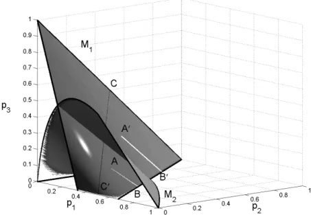
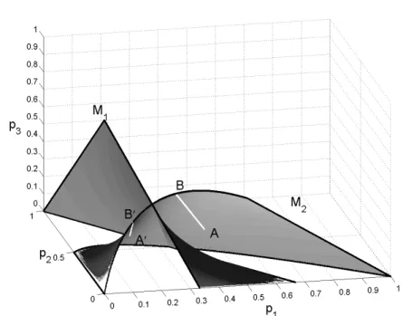
Figs. 1.4 and 1.5 present the two manifolds M1 and M2 in the space
C, C′on Fig. 1.4 corresponds to symmetric distributions for which p
2= p3. On
both figures, when starting the algorithm at x0 such that the point with
co-ordinates ([z0]21, [z0]22, [z0]23) is in A, to the even iterates z2k correspond points
that evolve along the line segment A, B, and to the odd iterates z2k+1
cor-responds the line A′, B′. The initial z
0 is chosen such that A is close to the
manifold M1 in Fig. 1.4 and to the manifold M2 in Fig. 1.5. In both cases
the limit set Z(x0) is a singleton {y} with n(x0, y) = 3: [y]3 = 0 in Fig. 1.4
and [y]2= 0 in Fig. 1.5.
Fig. 1.4. Sequence of iterates close to the manifold M1: A, B for z2k, A′, B′ for z2k+1; the line segment C, C
′
corresponds to symmetric distributions on M1 (p2 = p3)
1.4.2 A characterization of limit points through monotone sequences
Assume that x0is such that ν0has more than three support points. The limit
point for the orbit (zk) are such that rk+1= rk. To any y in Z(x0) we associate
the measure ν defined by ν(λi) = [y]2i, i = 1, . . . , d and then ν′ = Tν(ν) with
Tν given by (1.11); with ν and ν′ we associate respectively r(ν) and r(ν′),
which are defined from their moments by (1.26). Then, y ∈ Z(x0) implies
Tν[Tν(ν)] = ν and
∆(ν) = r(ν′) − r(ν) = 0 .
Fig. 1.5. Sequence of iterates close to the manifold M2: A, B for z2k, A ′
, B′ for z2k+1
Distributions that are symmetric with respect to µ1
When ν is symmetric with respect to µ1 direct calculation gives
∆(ν) = |M4,−1||M2,1| µ1|M3,0||M2,0|
,
which is zero for any four-point distribution. Any four-point distribution ν that is symmetric with respect to µ1 is thus invariant in two iterations, that
is Tν[Tν(ν)] = ν. The expression above for ∆(ν) is not valid when ν is not
symmetric with respect to µ1, a situation considered below.
General situation
Direct (but lengthy) calculations give ∆(ν) = N D with D = µ−1|M2,1||M2,−1|£|M1,0|2(|M1,−1||M4,1| − µ1|M4,−1|) + |M2,0|2(µ−1|M3,1| − |M3,−1|) − 2|M1,0||M2,0||M3,0|¤ (1.34) N = |M4,−1||M1,0|2£µ1(µ−1|M2,1| − |M2,−1|)2− µ−1|M2,1|2¤ +a2|M4,1| + b2|M3,−1| − 2ab|M3,0| (1.35)
with a = |M1,0||M2,−1| and b = (µ−1|M2,1| − |M2,−1|)|M2,0|. The
determi-nants that are involved satisfy some special identities
|M1,0|2= |M1,−1||M2,1| − µ1|M2,−1| (1.36) |M2,0|2= |M2,−1||M3,1| − |M2,1||M3,−1| |M3,0|2= |M3,−1||M4,1| − |M3,1||M4,−1| and µ−1|M1,1| − |M1,−1| = 1 , |M1,−1||M1,1| − µ1|M1,−1| = 0 (|M1,−1||M2,1| − µ1|M2,−1|)(µ−1|M1,1| − |M1,−1|) = |M1,0|2 (|M1,−1||M3,1| − µ1|M3,−1|)(µ−1|M2,1| − |M2,−1|) = |M2,0|2 +(|M1,−1||M2,1| − µ1|M2,−1|)(µ−1|M3,1| − |M3,−1|) (|M1,−1||M4,1| − µ1|M4,−1|)(µ−1|M3,1| − |M3,−1|) = |M3,0|2 +(|M1,−1||M3,1| − µ1|M3,−1|)(µ−1|M4,1| − |M4,−1|)
where all the terms inside the brackets are non-negative. Using these identities we obtain D = µ−1|M2,1||M2,−1| nh |M1,0|(|M1,−1||M4,1| − µ1|M4,−1|)1/2 +|M2,0|(µ−1|M3,1| − |M3,−1|)1/2 i2 + 2|M1,0||M2,0| × (|M1,−1||M3,1| − µ1|M3,−1|)(µ−1|M4,1| − |M4,−1|) (|M1,−1||M4,1| − µ1|M4,−1|)1/2(µ−1|M3,1| − |M3,−1|)1/2+ |M3,0| ¾
and thus D > 0 when ν has three support points or more. We also get a2|M4,1| + b2|M3,−1| − 2ab|M3,0| ≥ |M1,0|2|M2,1|2|M 3,1||M4,−1| |M3,−1| which gives N ≥|M1,0| 2|M 4,−1| |M3,−1| £|M1,0| 2(µ −1|M2,1| − |M2,−1|)|M3,−1| + |M2,0|3|M2,−1| ¤ ≥ 0 .
Now, y ∈ Z(x0) implies N = 0. Since |M2,−1| > 0 when ν has three
support points or more, N = 0 implies |M4,−1| = 0, that is, ν has three or
four support points only, and we recover the result of Theorem 8. Setting |M4,−1| = 0 in (1.35) we obtain that y ∈ Z(x0) implies
The condition (1.37) is satisfied for any three-point distribution. For a four point-distribution it is equivalent to b/a being the (double) root of the follow-ing quadratic equation in t, |M4,1| − 2t|M3,0| + |M3,−1|t2= 0. This condition
can be written as
δ(ν) = (µ−1|M2,1| − |M2,−1|)|M2,0||M3,−1| − |M1,0||M3,0||M2,−1| = 0 .
(1.38) (One may notice that when ν is symmetric with respect to µ1, δ(ν) becomes
δ(ν) = [|M1,0||M2,0|2/|M3,0|] |M4,−1| which is equal to zero for a four-point
distribution. We thus recover the result of Sect. 1.4.2.)
To summarize, y ∈ Z(x0) implies that ν is supported on three or four
points and satisfies (1.38). In the case of a four-point distribution supported on m, λj, λk, M , after expressing µ−1, µ4, µ5and µ6 as functions of µ1, µ2, µ3
though Z ti(t − m)(t − λ j)(t − λk)(t − M) ν(dt) = 0 , i ∈ Z , we obtain δ(ν) = KJ with K = 2α|M2,0| 3|M 1,0| mλjλkM p1p2p3(1 − p1− p2− p3) ×(λk− λj)2(λk− m)2(M − λk)2(λj− m)2(M − λj)2(M − m)2> 0 ,
where p1, p2, p3, α and J are defined as in Sect. 1.4.1. Since K > 0, the
attractor is equivalently defined by J = 0, which is precisely the situation considered in Sect. 1.4.1.
1.4.3 Stability
Not all three or four-point asymptotic spectra considered in Sect. 1.4.1 corre-spond to stable attractors. Although ν associated with some vector y on the unit sphere Sdmay be invariant by two iterations of (1.11), a measure νk
arbi-trarily close to ν (that is, associated with a renormalized gradient zk close to
y) may lead to an iterate νk+2far from νk. The situation can be explained from
the example of a three-point distribution considered in Fig. 1.3 of Sect. 1.4.1. The measure ν is invariant in two iteration of Tν given by (1.11). Take a
mea-sure νk= (1 − κ)ν + κν′ where 0 < κ < 1 and ν′ is a measure on (m, M ) that
puts some positive weight to some point λ∗ in the intervals (4/3, 161/108) or (1.7039, 1.9337). Then, for κ small enough the function Q2(t)Q′2(t) obtained
for ν′ is similar to that plotted for ν on Fig. 1.3, and the weight of λ∗ will
increase in two iterations since |Q2(λ∗)Q′2(λ∗)| > 1. The invariant measure ν
is thus an unstable fixed point for T2
ν when the spectrum of A contains some
eigenvalues in (4/3, 161/108) ∪ (1.7039, 1.9337). The analysis is thus similar to that in (Pronzato et al., 2001, 2006) for the steepest-descent algorithm (s = 1), even if the precise derivation of stability regions (in terms of the weights that two-step invariant measures give to their three or four support points), for a given spectrum for A, is much more difficult for s = 2.
1.4.4 Open questions and extension to s > 2
For s = 2, as shown in Sect. 1.4.1, if x0 is such that z0 is exactly on one of
the manifolds M1 or M2, then by construction z2k = z0 for all k. Although
it might be possible that choosing z0 close enough to M1 (respectively M2)
would force z2k to converge to a limit point before reaching the plane p3= 0
(respectively p2 = 0), the monotonicity of the trajectory along the line
seg-ment A, B indicates that there is no continuum and the limit set Z(x0) is a
single point. This was conjectured by Forsythe (1968) and is still an open ques-tion. We conjecture that additionally for almost all initial points the trajectory always attracts to a three-point spectrum (though the attraction make take a large number of iterations when zkis very close to M1∪ M2for some k). One
might think of using the asymptotic equivalence of rates of convergence, as stated in Theorem 5, to prove this conjecture. However, numerical calculations show that for any point on the manifold M1 defined in Sect. 1.4.1, the
prod-uct of the rates at two consecutive iterations satisfies Rk(W )Rk+1(W ) = r2∞
for any positive-definite matrix W (so that Rk(W )Rk+1(W ) does not depend
on p2 on the linear segment defined by r∞ on M1, see (1.32, 1.33), and all
points on this segment can thus be considered as asymptotically equivalent). Extending the approach of Sect. 1.4.2 for the characterization of limit points to the case s > 2 seems rather difficult, and the method used in Sect. 1.4.1 is more promising. A function ¯Qk
s(t) can be defined similarly to
(1.27), leading to two s-degree polynomials Qs(t), Q′s(t), see (1.28), each of
them having s roots in (m, M ). Let α and α′ denote the coefficients of terms
of highest degree in Qs(t) and Q′s(t) respectively, then α = α′ = 1/√q∞. Also,
let ω and ω′ denote the constant terms in Q
s(t) and Q′s(t); Theorem 5
im-plies that ωω′= 1/r
∞. Let n be the number of components in the asymptotic
spectrum S(x0, y), with s + 1 ≤ n ≤ 2s from Theorem 8; we thus have 2(s+1)
coefficients to determine, with n + 3 equations:
α = α′= 1/√q∞, ωω′ = 1/r∞ and Qs(λi)Q′s(λi) = 1 , i = 1, . . . , n
where the λi’s are the eigenvalues of A in S(x0, y) (including m and M , see
Theorem 9). We can then demonstrate that the functions Qs(t) and Q′s(t) are
uniquely defined when n = 2s and n = 2s−1 (which are the only possible cases when s = 2). When n = 2s, the system is over-determined, as it is the case in Sect. 1.4.1 for four-point asymptotic spectra when s = 2. The limit set Z(x0)
corresponds to measures ν for which the weights pi, i = 1, . . . , n − 1 belong to
a n−2-dimensional manifold. By setting some value to r∞or q∞the manifold
becomes (n − 3)-dimensional. When n = 2s − 1, ν can be characterized by its 2s − 2 first moments, which cannot be determined uniquely when s > 2. Therefore, although Qs(t) and Q′s(t) are always uniquely defined for n = 2s
and n = 2s − 1, the possibility of a continuum for Z(x0) still exists. The
1.5 Switching algorithms
The bound N∗
2 = (R∗2)1/2 on the convergence rate of the optimum 2-gradient
algorithm, see (1.21), is smaller than the bound N∗
1 = R1∗, which indicates
a slower convergence for the latter. Let ǫ denote a required precision on the squared norm of the gradient gk, then the number of gradient evaluations
needed to reach the precision ǫ is bounded by log(ǫ)/ log(N∗
2) for the optimum
2-gradient algorithm and by log(ǫ)/ log(N∗
1) for the steepest-descent
algo-rithm. To compare the number of gradient evaluations for the two algorithms we thus compute the ratio L∗
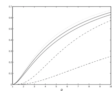
1/2= log(N1∗)/ log(N2∗). The evolution of L∗1/2as
a function of ̺ is presented in Fig. 1.6 in solid line. The improvement of the optimum 2-gradient over steepest descent is small for small ̺ but L∗
1/2tends to
1/2 as ̺ tends to infinity. (More generally, the ratio L∗
1/s= log(N1∗)/ log(Ns∗)
tends to 1/s as ̺ → ∞.) The ratio L∗
1/∞= log(N ∗
1)/ log(N∞∗), where N∞∗ is
defined in (1.22), is also presented in Fig. 1.6. It tends to zero as 1/√̺ when ̺ tends to ∞. 0 10 20 30 40 50 60 70 80 90 100 0 0.1 0.2 0.3 0.4 0.5 0.6 0.7 0.8 ρ Fig. 1.6.Ratios L∗
1/2 (solid line) and L ∗
1/∞(dashed line) as functions of ̺
The slow convergence of steepest descent, or, more generally, of the op-timum s-gradient algorithm, is partly due to the existence of a measure ν∗ s
associated with a large value for the rate of convergence R∗
s, see Theorem 4,
but mainly to the fact that ν∗
s is supported on s + 1 points and is thus
invari-ant in two steps of the algorithm, that is, Tν[Tν(νs∗)] = νs∗, see Theorem 3 (in
fact, ν∗
Switching between algorithms may then be seen as an attractive option to destroy the stability of this worst-case behavior. The rest of the paper is devoted to the analysis of the performance obtained when the two algorithms for s = 1 and s = 2 are combined, in the sense that the resulting algorithm switches between steepest descent and optimum 2-gradient. Notice that no measure exists that is invariant in two iterations for both the steepest descent and the optimum 2-gradient algorithms (this is no longer true for larger val-ues of s, for instance, a symmetric four-point distribution is invariant in two iterations for s = 2, see Sect. 1.4.2, and s = 3, see Theorem 3).
1.5.1 Superlinear convergence in R3
We suppose that d = 3, A is already diagonalized with eigenvalues m < λ < M = ̺m, and that x0is such that ν0puts a positive weight on each of them.
We denote pk = νk(m), tk = νk(λ) (so that νk(M ) = 1 − pk− tk). Consider
the following algorithm. Algorithm A
Step 0: Fix n, the total number iterations allowed, choose ǫ, a small positive number; go to Step 1.
Step 1 (s = 1): Use steepest descent from k = 0 to k∗, the first value of k
such that qk+1− qk< ǫ, where qk is given by (1.23) with s = 1; go to Step
2.
Step 2 (s = 2): Use the optimum 2-gradient algorithm for iterations k∗ to
n.
Notice that since qk is non-decreasing and bounded, see Theorem 6, switching
will always occur for some finite k∗. Since for the steepest-descent algorithm
the measure νk converges to a two-point measure supported at m and M ,
after switching the optimum 2-gradient algorithm is in a position where its convergence is fast provided that k∗ is large enough for t
k∗ to be small (it
would converge in one iteration if the measure were supported on exactly two points, i.e. if tk∗ were zero). Moreover, the 3-point measure νk∗ is invariant
in two iterations of optimum 2-gradient, that is, νk∗+2j = νk∗ for any j, so
that this fast convergence is maintained from iterations k∗ to n. This can be
formulated more precisely as follows.
Theorem 10.When ǫ = ǫ∗(n) = C log(n)/n in Algorithm A, with C an
arbitrary positive constant, the global rate of convergence Rn(x0) = · f (xn) f (x0) ¸1/n = Ãn−1 Y k=0 rk !1/n , (1.39)
with rk given by (1.14), satisfies
lim sup n→∞ log[Rn(x0)] log(n) < − 1 2.
Proof. We know from Theorem 6 that the sequence (qk) is non-decreasing and
bounded. For steepest descent s = 1 and the bound (1.24) is q∗
1= (M −m)2/4.
Since q0 > 0, it implies k∗ < (M − m)2/(4ǫ). Also, direct calculation gives
qk+1− qk = |Mk2,0|/qk2= |Mk2,0|/|Mk1,0|2 and, using (1.36), qk+1− qk= |M k 2,0| |Mk 2,1| 1 |Mk 1,−1| − µ1 |Mk 2,−1| |Mk 2,1| >|M k 2,0| |Mk 2,1| 1 |Mk 1,−1| , so that qk∗+1− qk∗ < ǫ implies |Mk∗ 2,0| |Mk∗ 2,1| < ǫ|Mk1,−1∗ | . (1.40)
For steepest descent, rk = |Mk1,−1|/(µk−1|M1,1k |) = 1 − 1/(µk1µk−1) < R∗1, so
that |Mk∗ 1,−1| = µk ∗ 1 µk ∗ −1− 1 < R∗1/(1 − R∗1) = (M − m)2/(4mM ) and (1.40) gives |Mk∗ 2,0| |Mk∗ 2,1| < ǫ(M − m) 2 4mM . (1.41)
The first iteration of the optimum 2-gradient algorithm has the rate rk∗ = f (xk∗+1) f (xk∗) = |M k∗ 2,−1| µk∗ −1|Mk ∗ 2,1| = |M k∗ 2,0| mM λµk∗ −1|Mk ∗ 2,1| , and using µk∗
−1 > 1/M and (1.41) we get rk∗ < Bǫ with B = (M −
m)2/[4M λm2]. Since d = 3, νk∗+2j = νk∗ and rk∗+2j = rk∗ for j = 1, 2, 3 . . .
Now, for each iteration of steepest descent we bound rk by R∗1; for the
optimum 2-gradient we use rk < Bǫ for k = k∗+ 2j and rk < R∗2 for k =
k∗+ 2j + 1, j = 1, 2, 3 . . . We have log[Rn(x0)] = 1 n ( log "k∗−1 Y k=0 rk # + log "n−1 Y k=k∗ rk #) . Since R∗
2< R∗1, Bǫ < R2∗for ǫ small enough, and k∗< ¯k = (M − m)2/(4ǫ) we
can write log[Rn(x0)] < Ln(ǫ) = 1 n ½ ¯ k log R∗1+ (n − ¯k) 1 2[log(Bǫ) + log(R ∗ 2)] ¾ . Taking ǫ = C log(n)/n and letting n tend to infinity, we obtain
lim
Algorithm A requires to fix the number n of iterations a priori and to choose ǫ as a function of n. The next algorithm does not require any such prior choice and uses alternatively a fixed number of iterations of steepest descent and optimum 2-gradient.
Algorithm B
Step 1 (s = 1): Use steepest descent for m1≥ 1 iterations; go to Step 2.
Step 2 (s = 2): Use the optimum 2-gradient algorithm for 2m2 iterations,
m2≥ 1; return to Step 1.
Its performance satisfies the following.
Theorem 11.For any choice of m1 and m2 in Algorithm B, the global rate
(1.39) satisfies Rn(x0) → 0 as the number n of iterations tends to infinity.
Proof. Denote kj = (j − 1)(m1+ 2m2) + m1, j = 1, 2 . . ., the iteration number
for the j-th switching from steepest descent to optimum 2-gradient. Notice that νkj−1 = νkj+2m2−1since any three-point measure is invariant in two steps
of the optimum 2-gradient algorithm. The repeated use of Step 2, with 2m2
iterations each time, has thus no influence on the behavior of the steepest-descent iterations used in Step 1. Therefore, ǫj= qkj− qkj−1 tends to zero as
j increases. Using the same arguments and the same notation as in the proof of Theorem 10 we thus get rkj < Bǫj for the first of the 2m2 iterations of the
optimum 2-gradient algorithm, with B = (M − m)2/[4M λm2]. For large n,
we write j = ¹ n m1+ 2m2 º n′ = n − j(m
1+ 2m2) < (m1+ 2m2). For the last n′ iterations we bound rk
by R∗
1; for steepest-descent iterations we use rk < R∗1; at the j-th call of Step
2 we use rkj < Bǫj for the first iteration of optimum 2-gradient and rk< R
∗ 2
for the subsequent ones. This yields the bound log[Rn(x0)] <
1
j(m1+ 2m2) + n′
× (
n′log(R∗1) + jm1log(R∗1) + j(2m2− 1) log(R2∗) + j X i=1 log(Bǫi) ) . Finally, we use the concavity of the logarithm and write
Pj i=1log(Bǫi) j < log à B Pj i=1ǫi j ! = log µ Bqkj − qm1−1 j ¶ < log µ Bq ∗ 1 j 
with q1∗ = (M − m)2/4, see (1.24). Therefore, log[Rn(x0)] → −∞ and
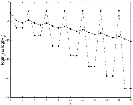
Fig. 1.7 presents a typical evolution of log(rk) and log(Rk), with Rk the
global rate of convergence (1.39), as functions of the iteration number k in Algorithm B when m1= m2= 1 (z0is a random point on the unit sphere S3
and A has the eigenvalues 1, 3/2 and 2). The rate of convergence rk of the
steepest-descent iterations is slightly increasing, but this is compensated by the regular decrease of the rate for the pairs of optimum 2-gradient iterations and the global rate Rk decreases towards zero.
0 2 4 6 8 10 12 14 16 18 20 −25 −20 −15 −10 −5 0 k log(r k ) & log(R k )
Fig. 1.7.Typical evolution of the logarithms of the rate of convergence rk, in dashed line, and of the global rate Rk defined by (1.39), in solid line, as functions of k in Algorithm B
Remark 7. In Theorems 10 and 11, n counts the number of iterations. Let n now denote the number of gradient evaluations (remember that one iteration of the optimum 2-gradient algorithm corresponds to two steps of the conjugate gradient method, see Remark 1, and thus requires two gradient evaluations), and define Nn(x0) = · f [x(n)] f (x0) ¸1/n (1.42) with x(n) the value of x generated by the algorithm after n gradient eval-uations. Following the same lines as in the proof of Theorem 10 we get for Algorithm A
log[Nn(x0)] = 1 n ( log "k∗−1 Y k=0 rk # + log "n−1 Y k=k∗ √r k #) < L′n(ǫ) = 1 n ½ ¯ k log R∗1+ (n − ¯k) 1 4[log(Bǫ) + log(R ∗ 2)] ¾ . Taking ǫ = C log(n)/n and letting n tend to infinity, we then obtain limn→∞L′n/ log(n) = −1/4.
Similarly to Theorem 11 we also have Nn(x0) → 0 as n → ∞ in
Algo-rithm B. ¤
The importance of the results in Theorems 10 and 11 should not be overem-phasized. After all, the optimum 3-gradient converges in one iteration in R3!
It shows, however, that an algorithm with fast convergence can be obtained from the combination of two algorithms with rather poor performance, which opens a promising route for further developments. As a first step in this direc-tion, next section shows that the combination used in Algorithm B still has a good performance in dimensions d > 3, with a behavior totally different from the regular one observed in R3.
1.5.2 Switching algorithms in Rd
, d > 3
We suppose that A is diagonalized with eigenvalues m = λ1 < λ2 < · · · <
λd = M = ̺m and that x0 is such that ν0 has n0 > 3 support points.
The behavior of Algorithm B is then totally different from the case d = 3, where convergence is superlinear. Numerical simulations (see Sect. 1.5.2) indicate that the convergence is then only linear, although faster than for the optimum 2-gradient algorithm for suitable choices of m1 and m2. A simple
interpretation is as follows. Steepest descent tends to force νk to be supported
on m and M only. If m1 is large, when switching to optimum 2-gradient,
say at iteration kj = j(m1+ 2m2) + m1, the first iteration has then a very
small rate rkj. Contrary to the case d = 3, νkj+2 6= νkj, so that the rate rk
quickly deteriorates as k increases and νk converges to a measure with three
or four support points. However, when switching back to steepest descent at iteration (j + 1)(m1+ 2m2) = kj+ 2m2, the rate is much better than the
bound R∗
1 since νkj+2m2 is far from a two-point measure. This alternation of
phases where νkconverges towards a two-point measure and then to a three or
four-point measure renders the behavior of the algorithm hardly predictable (Sect. 1.5.2 shows that a direct worst-case analysis is doomed to failure). On the other hand, each switching forces νk to jump to regions where convergence
is fast. The main interest of switching is thus to prevent the renormalized gradient zk from approaching its limit set where convergence is slow (since rk
is non-decreasing), and we shall see in Sect. 1.5.2 that choosing m1 = 1 and