Douuent Room , As any
<>arh
L~aco7-;* ~o° 'y oo ElectroeScCENTRIFUGAL DISTORTION IN ASYMMETRIC MOLECULES
II.
HDS
R. E. HILLGER M. W. P. STRANDBERG
OA J
TECHNICAL REPORT NO. 180
OCTOBER 5, 1950
RESEARCH LABORATORY OF ELECTRONICS
MASSACHUSETTS INSTITUTE OF TECHNOLOGYCAMBRIDGE, MASSACHUSETTS
-A
6
coQ
A&61~~~~~~~~~~~~~~~~~~~~~~~~~~'
The research reported in this document was made possible through support extended the Massachusetts Institute of Tech-nology, Research Laboratory of Electronics, jointly by the Army Signal Corps, the Navy Department (Office of Naval Research) and the Air Force (Air Materiel Command), under Signal Corps Contract No. DA36-039 sc-100, Project No. 8-102B-0; Depart-ment of the Army Project No. 3-99-10-022.
MASSACHUSETTS INSTITUTE OF TECHNOLOGY RESEARCH LABORATORY OF ELECTRONICS
Technical Report No. 180
CENTRIFUGAL DISTORTION II. October 5, 1950 IN ASYMMETRIC MOLECULES HDS R. E. Hillger M. W. P. Strandberg Abstract
A perturbation method for relating the theory of centrifugal distortion in asymmetric top molecules to observed microwave Q branch, a- or c-type transitions, is presented.
The formula for the distortion correction is expressed in terms of the total angular mo-mentum, J, the symmetry axis momentum of the nearest symmetric top, K, and five dis-tortion constants. The formula yields a satisfactory fit to the observed spectrum of HDS
(V - -0. 5). The electric dipole moment is determined as 1.02 + 0. 02 debye. The iner-tia defect and distortion constants are calculated. The effective structure for the HDS
molecule so determined is in agreement with infrared determinations.
I-CENTRIFUGAL DISTORTION IN ASYMMETRIC MOLECULES II. HDS
Introduction
The vibration-rotation energies of polyatomic molecules have been derived to a second order of approximation for special cases by a number of authors. In general, the method followed has been equivalent to that of Wilson and Howard (1). This work may be summarized by stating that the rotational term values of a molecule depend upon these quantities: the equilibrium structure of the molecule, the normal frequencies of vibration, and the nonvanishing coefficients of the anharmonic (cubic) terms in the ex-pression for the binding potential energy of the molecule. Nielsen (2) has calculated the matrix elements for the rotational energy including, to second order, vibration-rotation energies.
Unfortunately the correction of centrifugal distortion in asymmetric top rotational term values is, in general, an inconvenient process. The explicit diagonalization of the reduced energy matrix may be accomplished for only a relatively few low J terms, when the asymmetry coefficient and the six centrifugal distortion coefficients are included as unknowns. Since the experimental data are best used to evaluate the centrifugal distor-tion coefficients, the diagonalizadistor-tion of the reduced energy matrix for each trial value of these coefficients is awkward for comparison with experiment.
A method of arriving at an explicit form of the formula for centrifugal distortion correction terms to the rigid rotor frequencies has been demonstrated (3). This report will discuss a method of determining centrifugal distortion correction factors in terms of the general centrifugal distortion matrix elements.
1. Theory
The method used here is that of determining the centrifugal distortion correction in terms of rigid rotor frequencies specifically for Q branch a-type or c-type transitions.
This dependence may be determined explicitly in terms of quantum or pseudoquantum numbers and the rigid rotor absorption frequency by a modified application of conven-tional perturbation theory.
To review briefly, the reduced energy matrix is diagonal in J and M; the nonvan-ishing elements in K (i. e. Pz) are (K IHI K), (K IHI K ± 2), and (K IHIK ± 4). These
elements have been given by Nielsen (2) explicitly in terms of the molecular parame-ters.
The reduced energy matrix E(K) may be set up for a given value of J, the order of which is [(2J + 1)] since - J K< J. This matrix may immediately be factored to four
submatrices as in the case of the rigid rotor*. Explicitly these submatrices in terms *Obviously there is no loss in generality in considering only the reduced energy matrix,
since it contains the entire complexity of the asymmetric rotor problem. The addi-tion of [(a+c)/2] J(J+l) to E(K) yields the total energy.
of the original energy elements are
E+ =
a0 0 f2ao02 2a0 4 0
/2a02 a2 2 +a2,_2 a24 a26 °
F a0 2 4 a 44 a46 a48 0
0 I a2 6 a46 a66 a68 a6, 10
(1)
where E has the same elements as E+ after the first row and column have been deleted, and
al1- al,-1 1,-3 15 a +a al 30
1a3 1,-3 a33 35 37
a15 a35 a55 a57 a59 0
O a37 a57 a77 a79 a7,11
.. .. .. ... ... ...
(2)
In deriving these, use has been made of the relations
K, K = a-K,-K
aK, K+2 aK+2, K a-K, -K-2 = a-K-2, -K and
aK, K+4 aK+4, K a-K, -K-4 = a-K-4, -K (3) The matrices are presented in the general notation of King, Hainer and Cross (4) (here-inafter referred to as KHC) so that the identification of explicit energy levels is immedi-ately obtained from their work, and hence will not be duplicated here. The difference between KHC's matrices and those given above is that the latter give the entire energy of the molecule including distortion corrections.
The matrix elements for the rotational reduced energy are given explicitly by Nielsen* as
(KIHIK) = (R0 R+ 1K K + R3K ) (4)
*Nielsen's choice of phase factor for Px and P differ from KHC. We have modified Nielsen's results to agree with KHC by changing the sign of the (K I H IK + 2) elements. Either choice of phase yields identical results for the (K IHIK) and (KIHI K ± 4) ele-ments. In any case the modification is purely formal.
0+ =
(K IHIK + 2) = (J K +
l)1/2
R4 - R5 JK2 + (K + 2)2]} (5) (K IHIK + 4) =[f(J, K + 1)] [f(J, K+ ±3)]} '/R 6 (6) where R = F(- ) J(J+1) - DJ2 (J+1)2 R1 =e =r r R3 = -DK r RZ = (G-F) ( 2-) - DJK J(J+1) R4 = H(a-c) + J(J+1) f(J,n) = [J(J+1) - n(n-l)] [J(J+l) - n(n+l)] (7)and D, DJK,, DK' j, R5 and R6 are the six centrifugal distortion terms dependent upon the vibration frequencies and molecular structure parameters. R1 arises from
internal angular momentum and is hereafter neglected. a, b, and c are defined as the effective reciprocal moments of inertia of the molecule which when corrected for zero point vibration yield the equilibrium values, a e, be, and ce . * The latter are defined as the reciprocal moments of inertia the molecule would have if the atoms were located at the exact minima of the molecular binding potential, and may be expressed
h ae = 2 e cps b = cp ce = 8e rr Ic2e cps 8n 1 cc a>b> c . (8)
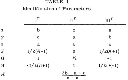
Plank's constant has been factored from all elements to reduce them to frequency units. The Ir representation is used for a-type Q branch transitions and the IIIr representation for c-type transitions. The actual definition of H, F and G in terms of a, b, and c are determined by the type of representation used. Table I has been prepared from KHC for this purpose. Further discussion of this point is given later.
*This is not quite correct, for there still remains a small correction due to vibration-rotation interaction which is dependent neither on vibration quantum number (zero point vi-bration) nor rotational quantum number (centrifugal distortion) i. e. Nielsen's xo, yo, and z .
----·I--·---TABLE I Identification of Parameters Ir IIr I I Ir x b c a y c a b z a b c F 1/2(K+) o G 1 K -1 H -i/2+) 1 2b-a-c a - c
In the Ir representation a-type transitions are between term levels of E and E-, or 0+ and 0-. Similarly for the IIIr representation, c-type transitions are given by the same selection rules.
The energy matrices (1) and (2) show clearly that the symmetric top K-degeneracy is removed in the Kt h level by a perturbation of order K. To illustrate, consider the E+ matrix. The 0+ level is a singlet level (nondegenerate in zero order). The 2+ level is split from the 2- level because of the second order coupling with the 0+ level through the off-diagonal elements Ta 0 2 . The term a,-2 is neglected for the moment since it is only a centrifugal distortion correction and small compared to the absorption energy. Both K = 2 levels are perturbed almost equally by the 4+ levels. So the K = 2 degeneracy is removed in second order. The 4 degeneracy is removed due to a second order
coupling with the 2 levels. Since the 2 degeneracy is removed in second order, the 4+ degeneracy is removed in fourth order, and so on. The degeneracy of the levels K+ and K- is thus eliminated in Kt h order due to the progressively greater splitting of the (K-2)+ and (K-4)', etc. levels.
Observation of this fact simplifies the calculation of the effect of including centrif-ugal distortion terms in the matrix. We postulate that the matrix has been progress-ively diagonalized by second order perturbation theory beginning with the next to the lowest K level in the matrix. Thus the new diagonal elements of the K-2 levels,
(aK2 K2)p, are assumed nondegenerate. The amount by which the levels are split is of course closely related to the absorption frequency vK_2. It differs slightly from the absorption frequency since the K± levels, which will eventually have their degeneracy removed, will further perturb the diagonal K-2 elements. The latter effect is taken
into account by writing* a
(aK-2, K-Z)p (aK-Z2 K-Z)p
K-
( aK, K-2 (9)*The rigid rotor frequency is not calculated so crudely, of course. Such an approxi-mation is only justified since we are interested in the additional contribution due to centrifugal distortion to an accuracy of a few percent.
This of course reduces to vK_2 in the region where second-order perturbation is appli-cable, i.e. where
2
aK, K-2 H f(J,K-l) << 1 (10)
(aK,K - aK-2, K-2) 64(G-F) (K-l)
By similar reasoning the interaction of the K level with the K + 2 level is negligibly small, thus 2 2 E! aKK-2 + K,K-4 (11) E+ (a+ a + (a+ aK K K-2, K-2)p aK,K K-4, K-4)p and hence 2 2 aK,K-2 aK,K-4 VK vK-2 aK + VK-4 (12)
VK VK2 (aK, K - aK-2, K-2) (aK, K- aK-4, K-4)
The term involving aK, K-4 is second order in a centrifugal distortion correction, and hence may be neglected.
The terms above are then written separating the rigid rotor contributions from the centrifugal distortion contributions.
26K, K-2 2 2(KK 6 K-2, K-2)
VK (VK)rigid (a ak + DK-2 (13)
aK-2
KK
-2, K-a)
where
aK, K-2 aK, K-2 (rigid) + (distortion), etc.
aK,K- raK, K-2 K, K-2
VK-2 =(VK-2)rigid (1 + DK-2)
and DK-2 is the centrifugal distortion contribution to vK_2 .
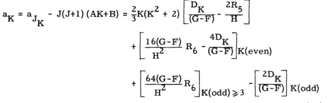
The term DK 2 is of course a similar term to that given above, but now in terms of DK 4 and so on. Finally, also, for low K values (1, 2, 3) the fourth off-diagonal terms, (K IH IK + 4), must be considered. When Eq. 13 is properly summed, using Eqs. 4, 5, 6 and 7, it may be written for odd and even K's as follows
(jK) (+ (VjK)6 + + (K-1) J(J+1) -F} (VJK)o ( K)r 1 2KJ(J+) fiJ + 3 K(K + 2) -
-
2 R6 ( KK(even ) + ~ H2 64(G-F) R 6 R[
. (14)H[ K(odd) >e 3 p K(odd) (14)
This is our desired equation.
It is well to reconsider the restrictions of this formula. First, one must stay away from the diagonal of perturbation divergence, i. e.
2
H f(J, K-l) << 1 . (15)
64(G-F)2 (K- )
Further discussion of this point is given in Ref. 3. Equation 14 is used to correct for the distortion in the observed microwave spectrum of HDS. Though this molecule is
quite asymmetric ( -' -0. 5) the convergence criterion given above is satisfied for the observable levels. It is to be noted, however, that though the convergence criterion is satisfied even for the observed high J high K lines, it may not be satisfied for the low K terms of the same J value. In other words, the convergence of a level JK may be assured, but the convergence of the splittings of the JK-2' JK-4' etc. may not be satis-factory. Such convergence is postulated in the derivation of Eq. 14. Since the distor-tion of the JK transidistor-tion is composed of its own terms, plus those of the lower order transitions, i. e. JK-2' JK-4' etc., each of these lower order contributions must be in turn calculable by this method to achieve Eq. 14. This is certainly not the case in
general. We only note that the contributions from the lower order K's diminish rapidly with decreasing K so that little error is caused as long as the main terms, the K - 2, and possibly K - 4 terms, meet the convergence requirement.
Second, it may be noted again that the above analysis is appropriate to Q-branch a-and c-type transitions. The type of transition covered is governed through F, G and H, by the representation used: Ir for a-type and III r for c-type transitions. The value of K in Eq. 14 corresponds to the KHC index K 1 or K+1 for a- and c-type transitions
respectively.
The restriction given above is not as drastic as may be first surmised, for mole-cules having significant distortion ("light" molemole-cules) and yet a microwave spectrum will, in general, satisfy it.
Finally, this analysis could be extended with more difficulty to P and R branches. At present such an extension seems of little general importance, since molecules with P or R branches in the microwave region will generally have large moments of inertia, and consequently small centrifugal distortion correction; or they will be nearly symme-tric tops, (only one small moment of inertia) and hence symmesymme-tric top formulae may be reasonably applied; or the qualitative analysis of Ref. 3 may also be used.
2. Centrifugal Distortion of HDS
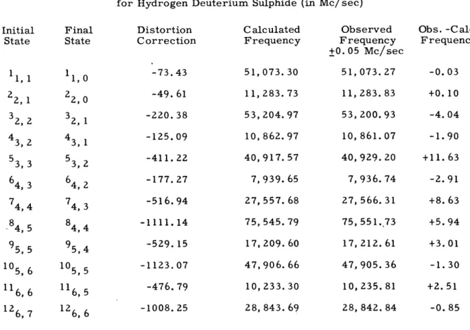
The experimental values of the rotational absorption frequencies of HDS , observed for the first time in the microwave region, and identified by the Stark effect, are given
in Table III. These data are now to be fitted to the distortion formula Eq. 14. The rigid rotor frequency is given by
(V JK)r = (a ) AE(()] (16)
-6-The process of fitting will be described briefly. A study of Eqs. 14 and 16 shows that there are seven adjustable parameters, i. e. the five distortion constants and (a-c)/2 and
K.
Fairly accurate values of the latter two constants are obtained from low J transitions. Assuming these are correct, the distortion constants are determined using the experimental frequencies and the method of least squares. The process is then reversed; vJ is calculated from the distortion constants just evaluated and com-pared with the observed (vJ ). Discrepancies are attributedtothefactthatthe (VJ , as determined from (a-c)/2 and /, are not exactly correct. Therefore, slight variations in (a-c)/2 andK
are made and the computations repeated until an entirely consistent set of results is obtained.The actual computations would seem to be quite laborious, but fortunately Eq. 14 lends itself to an analytical simplification which reduces the computations involved by a large factor. Taking values of (a-c)/2 and
K,
(vJ ) is calculated for each value ofJK. K in the present case is the KHC K_ 1 index for the asymmetric rotor. The differ-ences (jK) - (J) are taken and when finally the correct values of (VJK) are found, these differences will be the centrifugal distortion corrections. The following ratios
are formed for each line
aYJK (VJK)r
a (vJ | (17)
Now, if the differences a(J+l) aJK are taken between lines of equal K 1 the only distortion terms remaining are those which are a function of J. With slight rearrange-ment, a series of equations are obtained
a(J+1)K aJK DJK 2JK DJK
(J+ 1)- = T(G F) + 2TO K -P
= AK + B (18)
which represents a straight line as a function of K. The values of the constants A and B are taken as those which best fit this linear relationship and are found by the method of least squares. It turns out that if (a-c)/2 and
Ki
as chosen are almost correct, then the values of A and B are essentially independent of (vJK)r. Since (a-c)/2 and K are known to three-figure accuracy from low J transitions, the above computation need only be carried out once or twice during the process of fitting.A and B thus determine the J dependence of distortion and when substituted back into Eq. 14, a new series of equations are obtained, involving only K dependent and constant terms. These can be written
---·----22
Ft
DK
2R 5
aK = a - J(J+1) (AK+B) = K(K2 + 2) G- -aJK +l16(G-F) 4DK H 6 (G-F K(even) H K(odd) > 3 ( ) (19) where the "even" and "odd" notations indicate the terms which are present for even and odd values of K respectively. By taking the differences, aK+2 - aK, the coefficient of the K dependent term and the correct value ofK
may be determined. There are insuffi-cient data to evaluate all the constants unambiguously, therefore the value of DK is assumed to be known (see Sec. 4) since, in the case of HDS, it involves the smallest centrifugal distortion correction. Equation 19 for K = 1 then determines the value of (a-c)/2, R5 is calculable from the K-dependent term, and R6 results from the final remainder. It is at this point that the experimental data do not agree with the theory. The theory indicates that the remaining terms in R6 should show a four-to-one alterna-tion with K odd or even respectively, since DK/(G-F) is practically negligible. Experi-mentally, the remainder is a constant for any value of K > 2 for HDS. Since this disa-greement has not been resolved, the remainder, for purposes of fitting the experimental data, has been arbitrarily chosen to be [16(G-F)/HZ]R 6. Obviously, the constant terms become less and less important as J and K become large, i. e. for J = 12, K = 6, the three J and K dependent terms account for over 99 percent of the centrifugal distortion correction.The results of the equation fitting are summarized in Tables II and III.
TABLE II
N
, (a-c)/2 and Distortion Constants of Hydrogen Deuterium Sulphide (a-c)/2 = 3. 2664 cm 1 ] = -0. 47767 -4 -1 R5 = -2. 808 10 cm j = +2. 531 x 10 cm 1 -4 -1 D JK == +9. 133 x 10 cm DK = (-1.64 x 10- 4 cm-)* -5 -1 R6 = +0. 695 X 10 cm * Assumed.-8-TABLE III
Comparison of Calculated and Observed for Hydrogen Deuterium Sulphide (in
Distortion Correction -73.43 -49. 61 -220.38 116,6 116,5 126,7 126,6 -125.09 -411.22 -177.27 -516.94 -1111.14 -529.15 -1123.07 -476. 79 -1008.25 C alculated Frequency 51,073.30 11, 283. 73 53,204.97 10,862.97 40, 917.57 7, 939. 65 27, 557. 68 75, 545. 79 17,209. 60 47, 906. 66 10,233.30 28, 843. 69 Frequencies Mc/sec) Observed Frequency +0.05 Mc/sec 51,073.27 11, 283. 83 53,200.93 10, 861.07 40, 929.20 7, 936. 74 27, 566.31 75, 551.73 17, 212. 61 47, 905. 36 10,235.81 28, 842. 84 Obs. -Calc. Frequency -0.03 +0. 10 -4.04 -1.90 +11. 63 -2.91 +8. 63 +5.94 +3.01 -1.30 +2.51 -0. 85
The data presented in Table IV are quite consistent with no apparent systematic errors. For this reason, it is felt that the fitting is quite good and that the constants given in Table III truly represent the centrifugal distortion parameters of HDS.
3. Calculation of the Inertia Defect and the Effective Rotational Constants
The study of the rotational absorption spectrum of HDS yielded accurate values of (b-c) and (a-c)/2, but to obtain the effective rotational constants a, b, and c, another equation is required. If a AJ = +1 transition were observed and corrected for centrif-ugal distortion, the problem would be solved since (a+c) would then be' known. In the absence of this experimental data, one must resort to other means. Fortunately, another method is available because HDS is a planar molecule and hence the effective moments of inertia can be expressed in terms of the inertia defect , as follows
IV + IV -I = A
aa bb cc (20)
With a knowledge of the molecular force constants and vibrational frequencies obtained from infrared data, can be computed with a fair degree of accuracy. Since A is a
small correction term amounting to only a few percent of the rotational constants, an
-9-Final State 11, 0 2, 0 Initial State 1,1 22, 1 2, 2 43, 2 53, 3 64, 3 74, 4 84, 5 95, 5 105, 6 43, 1 53, 2 64, 2 74, 3 84, 4 95,4 105, 5
II_
__1_1_
_
_
_ _ _
I_ _I _ __ _CIIC_ _ _____Ierror as large as 10 to 20 percent may be permissible in the calculation of A and not affect the final results more than 1 percent. In addition, Darling and Dennison (5) and Nielsen (2) have pointed out that A is independent to second order approximation of the anharmonic force constants, and therefore only the harmonic terms in the potential energy function need be considered.
The necessary normal coordinates and vibrational frequencies are determined from existing infrared and Raman spectra data. The physical parameters of HDS are taken to be identical with HZS (6), an assumption which should be quite valid.
On the basis of Slater-Pauling valence forces, the kinetic and potential energy functions can be expressed directly in terms of the directed valence coordinates rl,
6r 2 and 6y which refer respectively to small displacements from equilibrium positions
in the sulphur-hydrogen bond length, the sulphur-deuterium bond length, and the angle y between the bonds, as pictured in Fig. 1. The energy equations are assumed purely
quadratic functions in the absence of knowledge concerning anharmonic terms.
The three Lagrangian equations of motion can be written immediately, and when solutions of the form et are assumed, the following secular equation is formed
Fig. 1. HDS molecules. 2 2 2 a kl a2 k 12 a13 X k13 al X -k a 2 X k a Xk k 12 k 12 a22 22 23 13 a X 13 23 k13 -a 33 2 - k 1 3 - a23 133-k a =0 (21)
where the X's are the normal frequencies (X = 4 c v ), the k's are force constants and the a's, reduced masses. The reduced masses are given explicitly by Cross and Van Vleck (7) for the general triatomic nonlinear molecule. The force constants were
assumed to be known from the work of Bailey, Thompson and Hale (8) on HZS and D2S;
thus the normal frequencies are determined for HDS. This assumption is quite valid in view of the fact that a comparison of the force constants of HZS and D2S shows
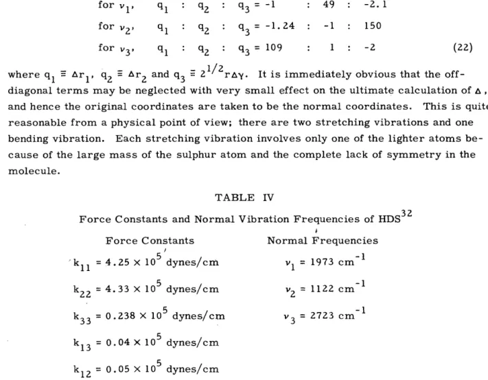
differ-ences of the order of magnitude of only one or two percent. The results seem quite reasonable considering the questionable infrared data on HDS. The force constants and zero-order frequencies are given in Table IV.
It is interesting to note that the off-diagonal terms of Eq. 21 are quite small, and thus the actual valence coordinates chosen are essentially the normal coordinates with minor corrections to be made due to the off-diagonal terms. The form of the normal vibrations compared with the original coordinates may be obtained directly from Eq. 21 and will be in the ratio of the first minors of any row in the determinant for each particu-lar normal mode of oscillation. These ratios turn out to be
-10-for v1 , ql : q2 : q3 = -1 for v2, q1 q2 : q3 = -1.24 for v3, q : q2 : q3 = 109 : 49 : -2. 1 : -1 150 1 : -2
where ql - rl, q2 Ar2 and q3 - 2 /2rAy. It is immediately obvious that the off-diagonal terms may be neglected with very small effect on the ultimate calculation of A, and hence the original coordinates are taken to be the normal coordinates. This is quite
reasonable from a physical point of view; there are two stretching vibrations and one bending vibration. Each stretching vibration involves only one of the lighter atoms be-cause of the large mass of the sulphur atom and the complete lack of symmetry in the molecule.
TABLE IV
Force Constants and Normal Vibration Frequencies of HDS3 2 Force Constants kll = 4.25 x 10⁵ dynes/cm k22 = 4.33 x 10⁵ dynes/cm k33= 0.238 X 10 dynes/cm k = 0.04 x 10⁵ dynes/cm kl2 = 0.05 x 10⁵ dynes/cm
Expressing the normal coordinates in state is computed to be Normal Frequencies v= 1973 cm I 1 =-1 V= 1122 cm 1 V= 2723 cm3 1
Nielsen's notation, for the ground vibrational
A = -0.244 X 1040 With A and the precise values of (b-c) of HDS are determined to be
and (a-c)/2, the effective rotational constants
a =9.682 cm 1; I = 2. 890 10- 4 0 gm-cm2 aa -1 v -40 2 b = 4.844 cm ; Ib bb 5.777x10 gm-cm c = 3. 140 cm- 1; IV = 8.910 x10-40 gm-cm- 2 cc (24)
These values can now be used in subsequent work, primarily to predict a AJ = +1 transition for the microwave spectroscopist and thus the complete experimental deter-mination of the effective rotational constants; and to present considerable aid to the infrared spectroscopist in the analysis of his data. It would be elegant to complete this
-11-(22)
2
gm-cm (23)
work by attempting to predict or calculate the equilibrium values of the moments of in-ertia, but the lack of knowledge of the anharmonic force constants, which give rise to the effects of the same order of magnitude as the effect of harmonic constants, makes this task impossible with any degree of accuracy.
4. Distortion Coefficients
The experimental distortion coefficients for HDS are given in Table II. These same coefficients can be calculated utilizing exactly the same data that were needed for the computation of a. Hence, the validity of the centrifugal distortion theory, of the calcu-lated effective rotational constants and of the structure of HDS can be quantitatively checked by computing these coefficients. The results of these calculations compared with the experimental values of the distortion constants are given in Table V.
TABLE V
Comparison of Calculated and Experimental Values of the Distortion Coefficients of HDS3 2
Distortion C alculated Experimental
Coefficient Value (cm-l) Value (cm- 1i)
R5 -2.Z1 x 10- 4 -2. 808 X10 - 4 -5 -5 6a +2.69X10- 10 +2.531X 5 DJK +9.16 X 10 4 +9. 133 X 10 4 DK -1. 64 X 10 4 (-1. 64 X 10-4)* R6 -1.90 X 10 5 +0. 695 10 5 DJ +8. 28 x 10 5 *Assumed.
While the results are not exactly perfect, the excellent agreement between the calcu-lated and measured values of the distortion constants exceeds expectations in view of the many simplifying assumptions made in the course of the previous work, and completes the cycle providing a check on the analysis presented in this report.
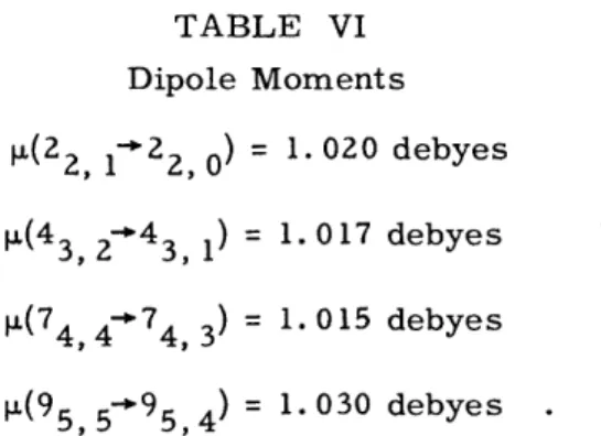
5. Stark Effect on HDS
The Stark effect was measured for four HDS lines, the 22 1 2 0; 43, 2-43 1; 74, 474, 3 and the 95, 595, 4' The dipole moment of each transition was computed with the results shown in Table VI. In all cases the Stark splitting follows a BM Z law where B is a constant depending on the transition. The contributions from terms involving
12-TABLE VI Dipole Moments ±(22, 1- 2 0) = 1.020 debyes 1(43 43 1) = 1.017 debyes 4(74, 474 3) = 1.015 debyes 1(95,5-95, 4) = 1.030 debyes
states other than the two participating in the absorption transition cancel to less than 1 percent of the major term value for all transitions except that for J = 2 where the contri-bution amounts to 1.2 percent. The latter correction is due entirely to the state J = 21 1 mixing with the J = 22 0 state.
Within the accuracy with which the measurements were made, the electric dipole moment of HDS is quoted to be
p = 1.02 + 0.02 debyes
It was originally thought that a correlation would be detected between a uniform change in [L and increasing J, i. e. increase of centrifugal distortion of the molecule. Such a change would indicate on the naive picture of a rotating molecule whether the hydrogen and deuterium were approaching or receding from each other. Unfortunately, the results are not accurate enough to discern such a trend. From an angular momentum point of view, i.e. (P) = aE/ai, it would seem that with incresing energy the dipole
moment should increase.
6. Absorption Coefficients and Isotopic Sulphur Transitions
The absorption coefficients in cm 1 of HDS3 2 absorption transitions are illustrated graphically in Fig. 2 as a function of the frequency in which form it serves several use-ful purposes. One, it presents all pertinent experimental data on HDS to the observer at a glance; two, experimentalists in the field may find the data useful as a standard; and three, qualitative predictions can be made regarding additional absorption transi-tions in HDS by observing the trends of the K families, as indicated by the light dotted lines on the graph.
Several absorption lines were observed and measured for the isotopic compounds HDS3 4 and HDS3 3, and these are tabulated in Table VII for future reference. The inten-sities of these lines are the same as shown in Fig. 2 but corrected for the natural abundance of the sulphur isotopes. The HDS3 3 line is the weakest line observed (a 10 7- cm ) and was the largest of three lines dispersed over a region of approxi-mately 10 Mc/sec. The poor sensitivity is not attributed to faulty equipment, but to a poor sample of HDS.
E o z z C.) z o z O z FREQUENCY IN KILOMEGACYCLES Fig. 2. HDS spectrum. TABLE VII Absorption Frequencies of HDS3 4 and HDS3 3 Transition 1 1,1 -1 1, 0 22, 1 22, 0 32,2 2, 1 43, 2 43, 1 74,4 4, 3 22, 1 22, 0 Frequency (Mc/sec) 50,912.27 11,235.45 52, 979. 67 10, 802.36 27, 392. 00 11,258.21 -14-C ompound HDS3 4 HDS3 4 HDS3 4 HDS3 4 HDS3 4 HDS3 3
7. Conclusion
Within certain restrictions a formula for centrifugal distortion in asymmetric
molecules has been presented. The distortion is determined by five calculable constants. As a test of the formula it has been applied to the observed microwave spectrum of HDS. The agreement is sufficiently satisfactory to confirm the general functional dependence of the formula on rotational state. Disagreement does exist, however, between the com-puted and observed effect both in magnitude and dependence of the contribution resulting from the fourth off-diagonal element, (R6). Fortunately the effect of this term is minor.
The formula given above compares with the approximate one derived in Ref. 3, except for a slight difference in the dependence on K. Further discussion of the com-parison of the two formulae will be given in paper III of this series.
References
1. E. B. Wilson, Jr., J. B. Howard: J. Chem. Phys. 4, 262, 1936 2. H. H. Nielsen: Phys. Rev. 60, 794, 1941
3. R. B. Lawrance, M. W. P. Strandberg: Centrifugal Distortion in Asymmetrical Top Molecules I: H2C12O, Technical Report No. 177, Research Laboratory of Electronics, M. I.T., Oct. 1950
4. G. W. King, R. M. Hainer, P. C. Cross: J. Chem. Phys. 11, 27, 1943 5. B. T. Darling, D. M. Dennison: Phys. Rev. 57, 128, 1940
6. P. C. Cross, G. W. King: Private communication
7. P. C. Cross, J. H. Van Vleck: J. Chem. Phys. 1, 357, 1933
8. C. R. Bailey, J. W. Thompson, J. B. Hale: J. Chem. Phys. 4, 625, 1936
-15-__