Symmetric Periodic Solutions in the N-Vortex Problem

HAL Id: tel-02462245

https://tel.archives-ouvertes.fr/tel-02462245

Submitted on 31 Jan 2020

HAL is a multi-disciplinary open access

archive for the deposit and dissemination of

sci-entific research documents, whether they are

pub-lished or not. The documents may come from

teaching and research institutions in France or

abroad, or from public or private research centers.

L’archive ouverte pluridisciplinaire HAL, est

destinée au dépôt et à la diffusion de documents

scientifiques de niveau recherche, publiés ou non,

émanant des établissements d’enseignement et de

recherche français ou étrangers, des laboratoires

publics ou privés.

Symmetric Periodic Solutions in the N-Vortex Problem

Qun Wang

To cite this version:

Qun Wang. Symmetric Periodic Solutions in the N-Vortex Problem. Fluids mechanics

[physics.class-ph]. Université Paris sciences et lettres, 2018. English. �NNT : 2018PSLED069�. �tel-02462245�

de l’Universit ´e de recherche Paris Sciences et Lettres

PSL Research University

Pr ´epar ´ee `a Universit ´e Paris Dauphine

Solutions P ´eriodiques Sym ´etriques dans le Probl `eme de N-Vortex

´

Ecole doctorale n

o

543

´

ECOLE DOCTORALE DE DAUPHINE

Sp ´ecialit ´e

SCIENCES

Soutenue par

Qun WANG

le 12 Dec 2018

Dirig ´ee par

Jacques F ´

EJOZ et Eric S ´

ER ´

E

COMPOSITION DU JURY :

M Alain CHENCINER Universit ´e Paris Diderot Pr ´esident

M Alberto ABBONDANDOLO Ruhr-Universit ¨at Bochum Rapporteur

M Thomas BARTSCH

Justus-Liebig-Universit ¨at Gießen Rapporteur

M Jacques F ´EJOZ Universit ´e Paris Dauphine Directeur de Th `ese M Eric S ´ER ´E

Universit ´e Paris Dauphine Codirecteur de Th `ese M Ke ZHANG

University of Toronto Membre du jury

Solutions Périodiques Symétriques dans

le Problème de N-Vortex

Qun WANG

Directeurs:

Prof. Jacques Féjoz

Prof. Eric Séré

préparé à l’Université Paris Dauphine

Université PSL

Une thèse soumise pour le diplôme de

Docteur en Sciences

2015t7月1Â/ÙŒ1873tÂe∞U0Ñ最ÌÑ7月1Â⇥_1/(Ÿ一)⌘•0ÜUniversit´e Paris IXÑ pf˚ZÎU÷⇢Â，1dÜœÜÇ同éÌ✏)一,pÊS›而 Ì≈éCÑ t⇥<d⇠√=öKˆ， ⌘ÛÅ⌘(Ÿ t-Ÿà⌘‡¡.©å◆±Ñ∫ÏÙÂ真⁄Ñ"✏⇥

ñH⌘Å感"⌘ÑZÎ生¸师Jacques F´ejozZÎåEric S´er´eZÎ⇥÷Ï⌃⌘引eÜpfvÑÜfl，v Ÿà⌘‡¡而ZöÑ/持å◆±⇥(Ÿ t-⌘Ïq同œÜÜ∏⇢qÕ4复åÛó±明⇥ $ˆ✏ã‰⌘ ∞∆Ò;⇥v一/Zå↵Jf期，⌘‡:(0ó一*˝œˆÿ∞⇤Q$*SobolevzÙÑLe8p，óK M一tJÑÂ\Mü=⇤⇥S´er´eYà)言◆±⌘Ù，S⌘Ï„≥不Ü一*pfÓòˆ，v不/⌘Ï‘ÍÒÛ a-Ù†‡˝，而/Ÿ*Óò‘Ûa-Ù† £⇥vå/(˚ZÎM⌘®‚F´ejozYàÑ✏¡，‚Ó⌘/& ÔÂœ8fi∞†a¢望ªP⇥F´ejozYàJ…⌘pfv(é思ÛKÍ1，ÇúL®˝不Í1，£H思Û谈 UÍ1⇥flè$M老师å⇣ZÎ∫á，不Ff0Üà⇢Â∆åπ’，Ùó0‰xæ^Ñv∂，Ÿ/⌘»生 ÑcxåPã⇥

⌘Å感"Alain ChencinerZÎ⇥H生一πb˘é SÓòŸà⌘¯⇢Ñ⌥¸，一πb˘-˝á化U ∞˙¯SÑg@åú1⇥,一!¡b，H生ø(-áJ…⌘÷ú1⇣◊，$1ãÙ“◊- ;，;- ◊”⇥H生˛(一«谈 û†±⌦)Sõf∞π’↵Ñá‡-– pf∂ô\ÑŒ<， 一µ'✏/Ù， ˚Hermiteᇉ∫感hG思ôÛÙÂ)外fiŸ，˚Poincar´eᇉ∫感h'SÛć^Ú≠·e⇥H生à ®⌥Poincar´e，一!⌘⌘ChencinerH生G•⌘sé˘hØ⇤ÑÂ\ˆ，H生Ó⌘˝&(Ä;ä¡明 思Ô˛“˙e，¡⌘flë*≥ø⌃⌃Y¸⌘ÅÒ;⌃êÄUÑ9,Ñ≈b，不ÅX</而^Ñ态¶⇥⌘Œ H生£Ãó0à⇢ÑY ⇥ ⌘Å感"Alain AlbouyZÎ⇥⌘ZÎ期Ù一Ë⌃ÑÂ\u感åheÍéAlbouyåKaloshin(¡明5SÓò -√Ñb P'Ñ一*引⌃⇥⌘‡d˘H生E·ÜÒÒÑ感¿⇥H生谈↵v不⇢e，Fá‡cÕºÂ˝Å :æ Bæ⇥\+⌦_⌦<4ÇwøJÌ↵Í2“:∫'˚=s”，H生¶ÔSK⇥ ⌘Å感"Bruno BouchardZÎ⇥⌘˛œ一¶:/&ûL;˚ZÎπk不≥⇥BouchardH生J…⌘7PI ªM~后ш⇡1ù一'„威ÎÃ⇥Ùe_Á，⌘60ÙŒ]'ZÎVf—⇢Âƈш⇡p}1/(ù 一ˆ12tÑ˘dU一¶Ω⇥

⌘Å感"ôÂ明ZÎ，Alberto AbbondandoloZÎ，Thomas BartschZ΢é⌘∫áÑ‘∆°⇧å–˙ Ñÿ5ÑÓ9✏¡，ŸÅ'Ñ–ÿÜ,áÑ(œ⇥=°1é⌘Ñ4s P，vÙæM ¯⇢∞✏，6而˘ é MYà不吝±9шÙ与æõ， (°?«↵-S∞Ñ∆Ùå%É，˝‰⌘Ò感cx⇥感" ÔZ Î不‹⌥ÃŒ⇢&⇢◆↵ve˙-⌘ÑZÎ’⇢T©‘X⇢⇥感"Igor BratusekH生(⌘T©ÑL?↵è-ŸàÑ.©åø)⇥

⌘Å感"$˙üZÎ，Eva MirandaZÎ，Alexey BorisovZÎ，Ivan MamaevZÎ，Alexander KilinZ Î，Urs FrauenfelderZÎ，Abed BounemouraZÎ，Amadeu DelshamsZÎ，Y˝ÕZÎ，u ZÎ，u KfZÎ，·! ZÎ，YчZÎ，Å⌘RZÎ，ø∏ZÎ，]f:ZÎ， zêZÎ，"—NZÎ， XøsÎ，⇠/)ZÎ，h贝†H生，įÖH生， ƒÏZÎ⌃´ÑÂ∆å˙Æ⇥÷Ï”ΩÜ⌘˘é® õ˚flå)SõfÑÜ„，v¿—Ü⌘à⇢∞Ñ思Ô⇥

⌘Å感"Patrick BernardZÎ，Yves MadayZÎ，R´emi RhodesZÎ，Olivier GlassZÎ，Stefano OllaZ Î，Pierre CardaliaguetZÎ，Otared KavianZÎ，YX´ZÎ，È^ZÎ，4pZÎ，êt˙ZÎ，Halim Doss ZÎ，Hans F¨ollmerZÎ，Chua Seng KeeZÎ，Jon BerrickZÎ，Chu DelinZÎ，Y∑0ZÎ，$  $ZÎ，Agnes SulemZÎ(⌘(ÙŒ,]'få∞†a˝À'f;˚UΫ↵-ŸàÑYÚ⇥

⌘Å感"HæZÎ，hπZÎ，ìURZÎ，Borrelli WilliamZÎ，Arnaud TriayH生, Michel OrieauxZ Î, Oms C´edricZÎ, Roisin BraddellsÎ，˘ZGH生，N星”H生，˘uusÎ，Charles BertucciZ Î，Clarke JorgeZÎ，Lafleche LaurentH生，Hannani AmiraliH生，_ôH生，êÔZÎ(ÙŒ,]' fÑCEREMADEû姟à⌘Ñj4，À≈，◆±å.©⇥ ⌘Å感" ffZÎ⇥⌘(f'˚fˆ,✏Œá，/H生Ñ0^ ⌫å谈⌘Œ生，⌘萌生Ü⇣:一* pf∂Ñ?望，最»⇤áŒ⌃p⌦ÜpfvKÔ⇥一Âfi»q'Í，H生引}E◆“Ze)2Í，˝n一 o‡”，∑∑与¯生q…，Ç fiÛwe一Ç(Â⇥ ⌘Å感"ãwõZÎ⇥Œ(∞†a˝À'f˚fw，wõ1一ÙŸà⌘Ì⌥Ñ.©⇥ŸÕ◆±一Ù持Ì 0⌘ZÎ’⇢⇥wõMN*¢，>Kï≥¶' Ê∫‰4>”KŒ⇥÷◆±⌘∫生(世，‡^“á明>æ ^，ŒÓ>SD”⇥⌘Ò◊感®，vÂdÍ…Û ⇥ ⌘Å感"-⌧flZÎ⇥Z:Íÿ-ˆ期Ñ⇢À，⌘Ï(l⌘pfvKM˝áœÜ‚ò⇥(⌦wpj jn∫S，Ù‰∫Îps生⇥⌧fl˛引⌦4_Ÿ.Œ4洞\↵⌘⌘，◆±⌘K—⌘⌦⇥vû~tK后，€ 'pfB◊ Â@⌦á‡，» ‡«˝够 世？¯‘K↵，⌧flDZfÓÑ«b，UØ，⇠≈，一言Â= K，“}C⌥∫>Ä„”，≥‰⌘»´Ò◊◆舞⇥ ⌘Å感" hH生⇥⌘ϯ∆é2011t，一同¡¡ÜhÙÑ∫ãÙÌåân≤"⇥ hH生Ñ✏û，§ 真，Ño，«b，I，˝‰∫感˘⇥ h˘⌘Ñ◆±åg~æÂ言h，⌘ÍBÍÒfÓ˝Ç h~f一 ,«猛æ€，π˝不ú负ŸM}↵ÀÑÀ≈⇥ ⌘Å感" ¸H生⇥ ¸H生不≈(‡U⌦与⌘œ8¢®，Ù/ÙŒpf与⌃∫i⌃Ñ-˝Zί生-最与⌘一¡ÇE⇧⇥œ Æ∫，ÄÄÒe⌘√⇥感ı¯∆é":，¢§é≤⇥，⌅né'w，fl?K—é i⌃，Ó´é‡U，⌘≤é_V⇥ ⌘Å感"Y6ZÎ⇥Y6H生œ8Ÿ⌘≤Üog（original generation ÑÇı，◆±⌘Œãü创Ñ \⇥v(intensive 500≠√Ü⌘ÑS⇥˝，/⌘˝够¨«ZÎ期Ù´√ãõÑÕÅ›¡⇥ ⌘Å感"u˝áH生⇥÷˘舞Hã⇢ÑÌ≈å˘[fÑT⁄˝ÒÒqÕÜ⌘⇥(⌘£ó£1ˆ，u˝á H生∞´Ù’，Âã3明“ÏÂ不{,®√:;”/—⌘>↵—Â外Ñ´外Ki，‰⌘ÒÒ◊(⇥ ⌘Å感"àπ， ’w+á⇥Œ’˝t⇢ˆLûL后，⌘与ŒMÑ同ã‡N≠ÜÄe，‡:⌘˘%+期 ÙÑá化á:不Â:6⇥àπ+á'π◊I，…vÇ«，Òó∞⌫¨æ^v- '⇥⁄6，“‚e°ûL S，{\°ûK∫”，⌘Õ?$ ÍÃÆ≥f^⇥ ⌘Å感"⇤ÅH生，àgsÎ，~#ÍsÎ， 33sÎ，*≈pH生，s君sÎ，N~ÖH生， ’ ssÎ，ã8‚sÎ˙-⌘ÑZÎT©∞:，:⌘Ù©威⇥ ⌘Å感"ÙŒN∫Ó⇤队ÑâÅ，Xwå，>Ì⌧，NÛ，4á*，uø，∑«，Ãv，7◊õ，Ø ˆ，õ≤，HP)，-~⇣，_o，Ì⇧，4k，刁z，⌦c，∑PR，ã✓*，0Œ，ãÒp ± ¿$老师⇥Ÿ/一*E·ƒ'(Ñ∆S，(à⇢‘[-⌘Ï_S˙Ü:låfiâ'⇥⌘ xj⇤队¶« Ü一µé}ˆI，v;ºÜSD，⇤ÇÜ´√⇥=°⌘œ8S∂，Ÿ⇤队&eªÊ，F/'∂ÕÁŸàÜ ⌘Ωπå/持⇥ 最后，⌘Å感"⌘Ñ6≤ãÙ‰H生，Õ≤÷明sÎ，å⌘ѪPãásÎ⇥""`Ï·›YÑ/持 å1⇥⌘䟫∫á.Ÿ`Ï，⌘最≤1Ñ∂∫Ï⇥ 2018t 月é∞†a

Résumé

Cette thèse porte sur l’étude des solutions périodiques du problème des N tourbillons à vorticité positive. Ce problème, formulé par Helmholtz il y a plus de 160 ans, possède une histoire très riche et reste un domaine de recherche très actif. Pour un nombre quelconque de tourbillons et sans contrainte sur les vorticit´s, ce système n’est pas intégrable au sens de Liouville : on ne peut trouver de solution périodique non triviale par des méthodes explicites. Dans cette th`se, à l’aide de méthodes variationnelles, nous prouvons l’existence d’une infinité de solutions périodiques non triviales pour un syst `me de N tourbillons à vorticités positives. De plus, lorsque les vorticités sont des nombres rationnels positifs, nous montrons qu’il n’existe qu’un nombre fini de niveaux d’énergie sur lesquels un équilibre relatif pourrait exister. Enfin, pour un système de N tourbillons identiques, nous montrons qu’il existe une infinité de chorégraphies simples.

Mots clés: système Hamiltonien, orbite périodique, N-Tourbillon, symétrie

Abstract

This thesis focuses on the study of the periodic solutions of the N-vortex problem of positive vorticity. This problem was formulated by Helmholtz more than 160 years ago and remains an active research field. For an undetermined number of vortices and general vorticities the system is not Liouville integrable and periodic solutions cannot be determined explicitly, except for relative equilibria. By using variational methods, we prove the existence of infinitely many non-trivial periodic solutions for arbitrary N and arbitrary positive vorticities. Moreover, when the vorticities are positive rational numbers, we show that there exists only finitely many energy levels on which there might exist a relative equilibrium. Finally, for the identical N-vortex problem, we show that there exists infinitely many simple choreographies.

Table of contents

List of figures vii

Nomenclature ix

1 Introduction 1

1.1 Vortex Model: From Continuum to Discrete . . . 1

1.1.1 Vortices Model in Hydrodynamics: Euler’s Equation . . . 3

1.1.2 Vortices Model in Quantum Mechanics: Gross-Pitaevskii Equation 4 1.2 From Integrable System to Non-Integrable System . . . 5

1.2.1 Integrable Cases . . . 5

1.2.2 Non-Integrable Cases . . . 9

1.3 Periodic Solutions of the N-vortex Problem . . . 11

1.3.1 Equilibria . . . 11

1.3.2 Non-Equilibrium Solutions . . . 15

1.3.3 Variational Method: From Poincaré to the Eight . . . 17

1.4 Variational Methods in the N-Vortex Hamiltonian Systems . . . 22

1.5 Main Results . . . 24

1.5.1 Periodic Orbits of the Positive N-Vortex Problem . . . 24

1.5.2 Choreographies of the Identical N-Vortex Problem . . . 26

1.5.3 An Uniform Bound Estimate for Symmetric Periodic Orbits . . . . 28

2 Periodic Orbits of the Positive N-Vortex Problem 31 2.1 Sparseness of Relative Equilibria . . . 32

2.1.1 Positive Vorticities . . . 32

2.1.2 Rational Positive Vorticities And Beyond . . . 34

2.2 Abundance of Non-Equilibrium Relative Periodic Solutions . . . 38

2.2.1 Symplectic Reduction and Relative Periodic Orbits in the Plane . . 38

3 Periodic Orbits of the Identical N-Vortex Problem 49

3.1 Absolute and relative choreographies . . . 53

3.1.1 (Simple) Choreographic Loop . . . 53

3.1.2 Reduced Choreographic Loop in CPN−1_{. . . . 54}

3.1.3 Centred Reduced Choreographic Loop in CPN−2 _{. . . . 55}

3.1.4 Relative choreographic loop in R2N _{. . . . 56}

3.2 Choreographic Holomorphic Spheres in Reduced Phase space . . . 58

3.3 Choreographic Fiber Bundle . . . 59

3.3.1 Choreographic Fiber and Section . . . 60

3.4 Choreographic Hamiltonian Perturbation . . . 61

3.4.1 Invariant Hamiltonian Under Choreographic Symmetry . . . 61

3.5 Well Posedness Of Choreographic Holomorphic Sphere . . . 63

3.5.1 Well Posedness of Choreographic Holomorphic Sphere . . . 64

3.6 Simple Relative Choreographies Of Planar Interactive Hamiltonian System 73 3.6.1 Simple Relative Choreography . . . 73

3.6.2 A Sufficient Condition For Existence Of Symmetric Component . . 76

3.7 Application To Some Physical Models . . . 76

3.7.1 The Non-Linear Discrete Schrödinger Equation . . . 77

3.7.2 The N-Vortex Problem in Hydrodynamics . . . 77

3.7.3 The N-Vortex Problem in Bose-Einstein Condensation . . . 80

3.7.4 Comparation With Other Methods . . . 84

4 Uniform Upper Bounds for Mutual Distances of Symmetric Periodic Solutions of N-Vortex Type Hamiltonian 87 4.1 Upper Bounds of Mutual Distances . . . 87

4.1.1 The Group of Italian Symmetry . . . 88

4.2 Uniform bound for Italian Symmetric T-periodic solution . . . 89

4.3 Application to Identical N-vortex System . . . 93

4.3.1 N-vortex System as Hamiltonian System . . . 93

4.3.2 Reparametrization Of Time . . . 93

4.3.3 Compactness for solution space of Floer Equation . . . 95

A Some Elementary Results on the Hamiltonian System 101 A.1 Poincaré-Melnikov Method . . . 101

Table of contents v B A minimax Approach For Identical N-Vortex Problem 105

B.1 Planar N-vortex Problem as Hamiltonian System . . . 105

B.1.1 Hamiltonian Structure and First Integrals . . . 105

B.1.2 Scatch of the proof . . . 107

B.2 The Existence of T-periodic solution for H2 . . . 107

B.2.1 Commuted Hamiltonian flows and the induced T-periodic solution of the Hamiltonian H1 . . . 112

B.3 Collision, Minimal Period and the Induced Periodic Solution of the Hamilto-nian H0 . . . 113

B.4 Symmetry and Exclusion of Collision . . . 116

B.4.1 Simple choreography . . . 116

B.4.2 Simple choreography with a center . . . 117

B.5 Verification of Palais-Smale condition . . . 118

B.6 Palais’ Principle and the Symmetry of choreography . . . 121

B.6.1 Symmetry of choreography . . . 121

List of figures

1.1 The Point Vortex Model of Helmholtz . . . 2

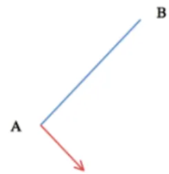
1.2 The velocity of A due to B, both with positive vorticity . . . 2

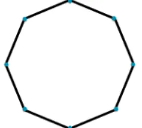
1.3 Thomson configuration for 8 vortices which form an octagon . . . 13

1.4 Figure "8" of the 3-body problem (picture taken from [33]) . . . 20

2.1 A non trivial relative periodic (left) coming from a non-centred relative equilibrium in the original phase space (right) . . . 39

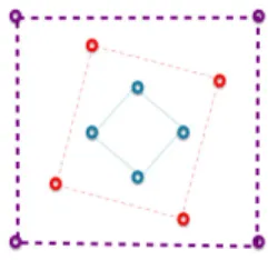
2.2 An example of a M ⇥ N-vortex configuration that is CN symmetric, with M=3, N=4 . . . 47

3.1 Two configurations of same H and I . . . 50

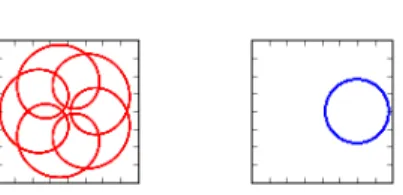
3.2 4-vortex problem in BEC restricted to Mρ . . . 83

3.3 A 3-polygon (equilateral triangle) in a rotational frame . . . 83

3.4 The configuration changing with reduced energy level . . . 85

B.1 The critical value is taken as the inf-sup among all the surfaces modelled on Q(left), thus is bounded above by sup on Q (right) itself . . . 112

Nomenclature

O(N, R) The Orthogonal Group

SO(N, R) The Special Orthogonal Group Sp(N, R) The Symplectic Group

U(N, C) The Unitary Group

HM The Hamiltonian on the symplectic manifold M

XH The Hamiltonian vector field of H

k•k The Norm

J The almost complex structure {•,•} The Poisson bracket

CPk The k-dimensional complex projective space R2N The 2N-dimensional Euclidean space Sk The sphere in k + 1 dimensional space

(M, ω) The symplectic manifold M with symplectic structure ω Hk The Hilbert Space Wk,2

Lp The Lebesgue’s Space

C∞ The Space of smooth functions Wk,α The Fractal Sobolev Space Wk,p The Sobolev Space

J The generlised momentum map Γi The vorticity of the i-th Vortex

z The 2N-dimensional vector describing the positions of N particles zi The 2-dimensional vector describing the position of the i-th particle

Acronyms / Abbreviations BEC Bose Einstein Condensation

NLDS Non Linear Discrete Schrödinger Equation

NNRPO Nontrivial Normalised Relative Periodic Solution NRPO Normalised Relative Periodic Solution

ODE Ordinary Differential Equation PDE Partial Differential Equation RPO Relative Periodic Solution RSC Relative Simple Choreography

Chapter 1

Introduction

1.1

Vortex Model: From Continuum to Discrete

The study of vortex dynamics has up to now 160 years of history, whose birth is marked by Hermann von Helmholtz’s seminal paper in hydrodynamics Über Integrale der hydro-dynamischen Gleichungen, welche den Wirbelbewegungen entsprechen[49], published in the year 1858.1 _{In his famous paper, Helmholtz has developped the conservation laws of}

vorticity for Euler’s model, which shows that the vorticity can neither be created or destroyed by any conservative forces. It is known today as the following theorems:

1. Helmholtz’s first theorem: The total vorticity flux in a vorticity tube remains constant along the tube;

2. Helmholtz’s second theorem: The total vorticity flux across any material surface remains constant in time2_.

In chapter 5 of his 1858 paper, by using these theorems, Helmholtz considered the perpendic-ular section of infinitely thin, straight, parallel vortex filaments with constant vorticity with a plane, thus he had introduced the point vortex model, known today as the N-vortex problem in the plane.

1_{It has been translated into English by Tait [86], and has shown considerable impact on the Victorian school} of hydrodynamics, including the development of vortex atom theory by William Thomson (more frequently mentioned as Lord Kelvin) [107–109] during the period 1867-1878.

Fig. 1.1 The Point Vortex Model of Helmholtz

Given a system of N vortices, each vortex zi= (xi, yi) with intensity Γi2 R \ {0}, their

dynamics are governed by the ODEs: ˙xi= − 1 2π

∑

_j6=i Γj |zi− zj|2(yi− yj), ˙yi= 1 2π

∑

_j6=i Γj |zi− zj|2(xi− xj) (1.1)

It is Kirchhoff who first has shown the Hamiltonian nature of this system in his lecture notes

Fig. 1.2 The velocity of A due to B, both with positive vorticity

on mathematical physics in 1876 [54]. More precisely, he had shown that the system could be written as Γid dtxi= ∂ ∂ yiH(z) Γid dtyi= − ∂ ∂ xiH(z) where H(z) = −_4π1

∑

1i< jN Γ_iΓ_{jlog |zi− zj|}2

1.1 Vortex Model: From Continuum to Discrete 3 Similar systems of point vortices have emerged from Bose-Einstein condensation to super-conductivity, from evolution of stellar system, to the geographical ocean flow. In this section, we give a brief discussion on the procedure of passing from continuum model to discrete model. It allows one to study infinite dimensional problems through an efficient finite dimensional approximation, and retrieve essential information on various phenomena in physics from simplified models.

1.1.1

Vortices Model in Hydrodynamics: Euler’s Equation

The motion of ideal incompressible flow is governed by the Euler’ equation

ut+ u · ∇u = −∇p (1.2)

Here u 2 R3_{represents the velocity vector field of the ideal fluid. Letting}

ω = curlu = ∇ ^ u = (∂yuz− ∂zuy, ∂zux− ∂xuz, ∂xuy− ∂yux), (1.3)

equation (1.2) becomes

Dω

Dt = ω· ∇u. (1.4)

By considering a very thin layer, we may assume that z = 0. The system is then 2-dimensional. For regularity considerations, we turn the above equation into the following weak form. Define

ωt( f ) = Z

Df (z)ωt(dz). (1.5)

We look for solutions ω(z,t) s.t. 8 < : d dtωt( f ) = ωt(u · ∇ f ) u(z,t) =R DJ∇GD(z, v)ω(dv).

Here f : D ⇢ R2_{! R}2_{is a bounded smooth function, and G}

Dis the Green function in domain

D. We are interested in the evolution of point vortices in the whole plane. In this case, • The initial vorticity function is the following point vorticity distribution:

ω0(dz) =

∑

1iN

• D = R2_{, and G}

D(z, v) = − 1

2πlog |z − v|.

Observe (by using a regularizing sequence if necessary) that a vortex is at rest under the action of its own field due to symmetry. We finally arrive at the following system:

8 < : Γ_idtdxi=_{∂ y}∂_iH(z) Γi_dtdyi= −_{∂ x}∂_iH(z), 1  i  N, where H_R2N(z) = − 1 4π_{1i< jN}

∑

ΓiΓjlog |zi− zj| 2 _(1.7) By taking Xi=p|Γi|xi,Yi= Γip|Γi|yi (1.8)

the above system becomes a standard Hamiltonian system.

In this thesis we will not focus on the impact of a boundary on the dynamical behavior, we only mention that in the presence of a boundary the Hamiltonian is more complicated, i.e.,

HΩ(z) = − 1 4π_{1i< jN}

∑

ΓiΓjlog |zi− zj| 2₊

_∑

1iN RΩ(zi) (1.9)

It consists of two parts: the Kirchhoff function H_R2N, which rules the interactions between

vortices; and the Routh function RD, which depends on the Green function of the domain Ω,

and which evaluates the interaction of each vortex individually with the boundary ∂ Ω. In some situations, RΩcould be found explicitly by using the so-called image method. For a

general discussion, see Lim [62].

1.1.2

Vortices Model in Quantum Mechanics: Gross-Pitaevskii

Equa-tion

Consider a dilute gas of bosons that is cooled to an extremely low temperature near absolute zero. Normally, atoms will present different macroscopic wave functions. However in this extreme situation, all the atoms will present a single macroscopic wave function. This state of matter is called Bose-Einstein Condensation (BEC). The wave function ψ of the

1.2 From Integrable System to Non-Integrable System 5 cloud of atoms is described by a partial differential equation(PDE), i.e., the Gross-Pitaevskii (GP) equation:

i∂tψ = −1

2∆ψ +V (x, y)ψ + |ψ|

2_{ψ (1.10)}

Here V (x,y) is the function describing the artificially set external potential(magnetic and optic fields), which is used for confining the atoms. In practice, V (x,y) is taken to be isotropic about the origin, and is realized either via a harmonic trap [41] or via a hard wall container [3]. Note that when V = 0, it is the classical cubic Schrödinger equation. Again we could consider the interaction of straight vortex lines and write a ODE system as an approximation of this PDE system. It turns out that the governing Hamiltonian becomes

H(z) = −1₂(µ N

∑

i=1 log 1 1 − |zi|2+ λ

∑

_{i< j}log |zi− zj| 2_{) (1.11)}

In this case the vortices are confined in the unit disk. As in the bounded domain N-vortex prob-lem in hydrodynamics, these vortices intersect pairwise with each other, and, simultaneously, individually with the boundary.

1.2

From Integrable System to Non-Integrable System

The Hamiltonian nature of the N-vortex problem opens the door to using symplectic methods, and naturally raises the question of integrability. Integrability is one of the first important qualitative features of a Hamiltonian system. It implies the existence of a regular invariant foliation, thus excludes the possibility of chaotic behavior. Moreover, integral curves may be found by means of quadratures and eliminations. To the contrary, the non-integrable Hamiltonian system is in general much harder to understand. In this chapter, we take N-vortex problem from hydrodynamics as our example, and review some known results about the integrability of the N-vortex problem. It turns out that for N  3 the system is completely integrable, while for N > 4 it is in general non-integrable.

1.2.1

Integrable Cases

In this subsection, we recall the definition of Liouville integrability, and show that the 3-vortex problem from Euler’s equation is an integrable Hamiltonian system. Similar analysis applies to 2-vortex problem from BEC.

Liouville Integrablity

Let (M,ω) be a symplectic manifold, where M = R2N, ω = N

∑

i=1 1 Γidyi^ dxi

is the vorticity-weighted symplectic structure. The N-vortex problem could then be writen as Γ˙z = XH(z)

Definition 1.2.1_{(Poisson Bracket). The Poisson Bracket of two functions F,G 2 C}∞(M, R) is defined as

{F,G} = ω(dF,dG) (1.12) In our case, in local coordinates the Poisson Bracket can also be interpreted as

{F,G} =

∑

1iN 1 Γi( dF dxi dG dyi− dF dyi dG dxi) (1.13)

It is easy to check that the following properties holds for the Poisson Bracket

{F, µ1G + µ2H} = µ1{F,G1} + µ2{F,H}; (bi-linearity)

{F,G} = −{G,F}; (skew-symmetry) {F,GH} = G{F,H} + H{F,G}; (Leibniz rule) {{F,G},H} + {{G,H},F} + {{H,F},G} = 0 (Jacobi Identity) Definition 1.2.2(First Integral). A function F 2 C∞(M, R) is called a first integral of the Hamiltonian system if {F,H} = 0.

The following theorem on Liouville integrability is taken from [9].

Theorem 1.2.1(Integrable System). Suppose that we are given N functions on a 2N- dimen-sional symplectic manifold, h = (h1, h2, ..., hN) 2 RN, and

Lh= {z 2 M| Fi(z) = hi, 1  i  N} (1.14)

If they satisfy moreover that

1.2 From Integrable System to Non-Integrable System 7 • Fi, 1  i  N are independent on Lh, i.e. det(dFdz) 6= 0 on Lh

Then

1. Lhis an smooth manifold invariant under the flow φHof the Hamiltonian.

2. If further more Lhis connected and compact, then Lhis diffeomorphic to TN

3. There exists so-called action angle variables (I, φ ) s.t. under this symplectic transfor-mation the flow of the Hamiltonian flow is quasi-periodic:

˙

φ = ωh, ωh= ω(h) 2 RN (1.15)

4. The canonical Hamiltonian equation can be integrated by quadratures. Integrability of N-Vortex Problem:_{N  3}

The first three integrals of the N-vortex problem have first been found explicitly by Henri Poincaré in [88]. Note that

• The system is invariant under translation,hence P(z(t)) =

∑

1iN

Γixi(t) = cst, Q(z(t)) =

∑

1iN

Γiyi(t) = cst (1.16)

• The system is invariant under rotation,hence I(z(t)) =

∑

1iN

Γ_i|zi(t)|2= cst (1.17)

It turns out that

{H,I} = {H,P2+ Q2} = {P2+ Q2, I} = 0 (1.18) As a result the 3-vortex problem is integrable and much about it has been understood since a long time. In 1877, Gröbli in his dissertation [44] has first introduced the relative coordinates represented by the mutual distances ρ12, ρ23, ρ13between the three pairs of vortices. Using

these coordinates, he has re-calculated the first integrals, and investigated in particular problems today known as the relative equilibria and the self-similar motions. In 1949, Synge [105] has reinvestigated the problem using the same coordinates, and analyzed the stability of relative equilibria. He has also found different relative periodic solution configurations. Some

general observation on discrete symmetry of the system has also been discussed therein. Later on Novikov [78] has use the phase diagram technique to classify possible motion regimes for 3 identical vortices, followed by the generalisation to 3-vortex problem with arbitrary vorticities by Aref [5]. Poisson geometric aspect of 3-vortex problem is studied by Borisov et al in a series of papers [23, 20, 21].

Symplectic Reduction and Reduced Hamiltonian

Before we enter into the discussion for periodic solutions of the N-vortex problem, let’s first notice that closed orbits of N-vortex problem of hydrodynamics are not isolated. Indeed, if z(t) is an orbit, then so are

• (z1(t) + c, ··· ,zN(t) + c), c 2 R2;

• (eiθ_z

1(t), ··· ,eiθzN(t)), θ 2 R \ 2πZ;

• λ12z(_λt), λ > 0.

We wish not to distinguish such orbits, thus introducing the following definition. Definition 1.2.3. We will call an orbit z(t)

• centred if it satisfies P(z(t)) = Q(z(t)) = 0 ; • normalized if it is centred and satisfies I(z(t)) = 1 ; • periodic if z(t) = z(t + T ) for some T > 0 ;

• relatively periodic orbit (RPO) if z(t) = gz(t + T ) for some T > 0 and g 2 E(2). Thus, (NRPO) will stand for a normalized relative periodic orbit, and this is the object that we want to study. For the N-vortex problem in BEC, although the scaling and translation in general does not give new solutions, the system is still invariant under rotation while we are more interested in studying the deformation rather than the rotation of the configuration. For these purposes, we would like to study the projected flow of the system on some quotient manifold, which represents the truly deformation of the configuration. In Appendix A we have recalled briefly the theory for symplectic reduction and the reduced Hamiltonian, which serves exactly our need.

1.2 From Integrable System to Non-Integrable System 9 • N-Vortex Problem of Hydrodynamics:

The system is invariant under the action of the special Euclidean group SE(2), the phase space is CPN−2_{, as is shown in the following diagram:}

S1

R2N R2N−2 S2N−3

CPN−2

p=q=0 I=1

/SO(2)

• N-Vortex Problem of Bose-Einstein Condensation:

The system is invariant under the action of the special orthogonal group SO(2), the phase space is CPN−1_{, as is shown in the following diagram:}

S1 R2N S2N−1 CPN−1 I=1 /SO(2)

1.2.2

Non-Integrable Cases

Analysis of the N-vortex problem for N ≥ 4 is in general quite difficult, because there is not enough first integrals in involution to give a solution explicitly by quadratures. In this section, we investigate two aspects of the dynamical behavior of some special N-vortex problems, which could somehow be seen as nearly integrable Hamiltonian systems. On one hand, the application of Poincaré-Melnikov method reveals the chaotic behavior of the system; on the other hand, the application of Kolmogorov-Arnold-Moser theory ensures the stability of invariant tori.

Chaotic Behavior of N-vortex Problem:_{N ≥ 4}

In this subsection, we review the detection of chaotic behavior of N-vortex problems by the Poincaré Melnikov method.

There has been a couple of analytic proofs of the non-integrability of the 4-vortex problem based on the Poincaré-Melnikov method. In general, one assumes that one or more of the vortices have zero vorticity, hence they are particles under influence of the large vortices. This idea is somehow similar to the restricted 3-body problem in celestial mechanics. As the zero vorticity is turned into small but positive vorticity, the system will trigger the homoclinic chaos.

1. Ziglin’s configuration

In 1980, Ziglin first proved the non-integrability of 4-vortex problem by considering a perturbation of the equilateral triangle configuration [121]. The configuration envolves essentially a passive particle in the vector fields generated by a equilateral triangle formed by 3 identical vortices. Based on Ziglin’s method later on Bagrets and Bagrets have proved the non-integrability of 4-vortex problem on the sphere [11].

2. Koiller and Carvalho’s configuration

Koiller and Carvalho’s proof for the non-integrability of the 4-vortex problem in 1989 [55] has chosen a different configuration. where two vortices with opposite vorticity Γ_{1= −Γ2}will have impact on the passive particles Γ3= Γ4= ε << 1.

3. Castilla, Moauro, Negrini, and Oliva’s configuration

Castilla et al have considered another configuration to show the non-integrability of the 4-vorte problem in 1993 [27]. It consists of 3 identical vortices of vorticity 1 and a 4th_{passive vortex of small vorticity 0 < ε << 1. Their configuration could be seen}

as a perturbation of the heteroclinic orbits of Euler’s configurations between different permutations.

Stable Behavior of N-vortex Problem:_{N ≥ 4}

We have already seen in the previous section that for an integrable Hamiltonian system, its phase space up to a symplectimorphism, is foliated by Lagrangian invariant tori. The dynamics on these tori are quasi-periodic. The Kolmogrov-Arnold-Moser theory deals with the stability of these tori: it implies that, under suitable assumptions, for the perturbed Hamiltonian system (which are nearly integrable Hamiltonian systems) these tori persist. For brief introduction of KAM theory, see J.B.Bost [24] and [40] for application to celestial mechanics. The first application of KAM theorem to N-vortex problem is given by Khanin in 1982 [53] , who has shown that for general N-vortex with arbitrary vorticity Γi2 R \ {0},1 

i  N, there exists a set of initial conditions of positive measure, for which the motion of vortices is quasi-periodic. While the existence result is established, little is known about

1.3 Periodic Solutions of the N-vortex Problem 11 the size of perturbation admissible for such tori to survive. In 1988 Alessandra Celletti and Corrado Falcolini [28] has shown that a lower bound of perturbation size could be εKAM = 7.81 ⇥ 10−23 for a prescribed frequency ω =

p 5−1

2 . Lim [64] has studied the

existence of KAM tori for vortex lattice. Blackmore and Knio [18] have studied various KAM type results for three coaxial vortex rings.

1.3

Periodic Solutions of the N-vortex Problem

As mentioned in the last section, the N-vortex problem is in general not integrable when N > 3. This is somehow similar to the case of 3-body problem in celestial mechanics, which serves as one of the main resources for the modern development of dynamical systems. The singularities at collision and at infinity which put considerable difficulties from the analytical point of view, could be overcome by the construction of periodic solutions. Moreover, in Poincaré’s mind, these solutions are also building blocks of general motions of the 3-body problem, as he believes one can use them to approximate any solutions. Actually, Poincaré has pointed out in his revolutionary monograph of celestial mechanics the significance of (relative) periodic solutions:

D’ailleurs, ce qui nous rend ces solutions si précieuses, c’est qu’elles sont, pour ainsi dire, la seule brèche par où nous puissions essayer de pénétrer dans une place jusqu’ici réputée inabordable.

We believe the same philosophy applies to the N-vortex problem too. Thus in this section, we will discuss some of the results in the study of periodic solutions for the N-vortex problem.

1.3.1

Equilibria

Absolute Equilibria

Equilibria may appear either in an inertial frame or in some rotating frame. In the former case, these solutions are called absolute equilibria (fixed points), while in the later case they are called relative equilibria.

The 3-vortex problem cannot have any fixed point unless the following conditions are fulfilled simultaneously [44, 105]

z2− z1=

Γ2

Γ₃(z1− z3)

Then O’Neil [79] has studied the general case and concluded that the corresponding necessary condition for the existence of an absolute equilibrium is that the total angular momentum vanishes:

L =

∑

1i< jN

ΓiΓj= 0 (1.20)

Moreover, the converse is almost true: given almost all choices Γ = (Γ1, Γ2, ..., ΓN) s.t. L = 0,

there exists exactly (N − 2)! different absolute equilibria. Recently, Bartsch, Micheletti and Pistoia have studied the existence of fixed points for the planar N-vortex problem in a bounded domain, together with their non-degeneracy [15, 14]. In particular, they have shown that the Kirchhoff-Routh function being Morse is a generic property. Kuhl has shown under some technical assumption the existence of the collinear equilibria and possible symmetry [58, 57].

Relative Equilibria

There exists much more intensive study for relative equilibria, especially those becoming fixed point in a rotating frame. Such notion exists in celestial mechanics. These configurations correspond to a larger category of configurations, i.e., the central configuration in celestial mechanics [70]. However due to the fact that for N-vortex problem the phase space coincides with the configuration space, the notion of central configurations and relative equilibria coincide in N-vortex problem. We assume that the total vorticity ∑_1iNΓi6= 0, as a result

the vorticity center is finite. The relative equilibrium configurations in the N-vortex problem could be defined as the following:

Definition 1.3.1. A periodic solution of the planar N-vortex problem is called a relative equilibrium, if it is of the form

zi(t) = eJωt(zi(0) −C) +C

where C is the vorticity center.

We list some properties that will be used frequently later on: Proposition 1.3.1. The following are equivalent:

(1) z 2 Z1; (1.21)

1.3 Periodic Solutions of the N-vortex Problem 13

Fig. 1.3 Thomson configuration for 8 vortices which form an octagon

Proof. _{: (1)) (2) : By definition of relative equilibrium, z(t) 2 Z}1implies 9ω 2 R s.t.

∇H(z(t)) =ω

2∇I(z(t))

taking inner product with z(t) on both sides. Since I(z) = 1, one sees that −_2πL = ωI(z(t)) )ω₂ = −_4πL

Hence (2) is proved.

(2)) (1) : If z satisfies that ∇H(z) = −_4πL ∇I(z), then the flow passing through z will be a relative equilibrium. We need to show that such a relative equilibrium is normalized. First, by considering (x,y) 2 R2_{as a complex number x + iy 2 C, (3.18) implies that}

−_2π1

∑

j6=i ΓiΓj ¯zi− ¯zj |zi− zj|2= − L 4πΓi¯zi, 81  i  N It follows that 0 = −_2π1 N

∑

i=1

∑

j6=i ΓjΓi ¯zi− ¯zj |zi− zj|2 = − N

∑

i=1 L 4πΓi¯zi Thus ∑N

i=1Γizi= 0, and z is centred. Next, multiply z on both sides of (3.18), so that

−_2πL = ∇H(z)z = −_4πL ∇_{I(z) z = −}L

2πI(z). Thus I(z) = 1.

The study of relative equilibria comprises various aspects, for instance the explicit con-struction of solutions, or the finiteness of configurations for given or generic vorticities, etc.

Explicit construction of relative equilibria Historically, the first such solution is the reg-ular N-polygon rotating around its center. This configuration first appears in the work of J.J.Thomson [106] and is known as Thomson’s configuration since then. Staring from this point, Havelock [48] has found the double vortex ring which is named after him too. Aref [6] and Koiller et al [56] has studied the case of relative equilibria with a center of symmetry, which is later on generalized by Lewis and Ratiu [60] for cases of sub-rings with different vorticity. For a comprehensive study of these vortex rings and multi-rings, one could turn to [7], which discussed not only such relative equilibria in the plane but also on the sphere, and even on various two dimensional manifolds. There exists relative equilibria which are not symmetric, as Aref and Vainchtein have shown by the method of continuation [8].

Finiteness of relative equilibria Relative equilibria of the N-vortex problem are in general not isolated due to the invariance under translation and rotation. After the normalisation, it turns out that the above defining equation represents a rather complicated system of algebraic equations, depending on the N vorticities. With the preassumed vorticities, the solution set of these equations is an algebraic subset of the product space of the phase space. This is quite similar to the situation of celestial mechanics, where the finiteness of central configuration of Newtonian gravitational systems, known as the Smale’s 6th_{problem for 21st century [101],}

is only solved in the first simplest cases and remains as a challenge. O’Neil has shown in [79] that when ∑_{1i< jN}ΓiΓj6= 0,∑_1iN6= 0, there are no more thann!₂ collinear relative

equilibrium configurations. Hampton and Moeckel [47] have shown the finiteness of the number of relative equilibria configurations for N = 4 is generic by using similar methods in their earlier work for 4-body problem [46]. More precisely, they have shown that

Theorem 1.3.1(Theorem 1.[46]). Let L = ∑_{1i< jN}ΓiΓj, Γ = ∑_1iNΓi. If the vorticities

Γiare nonzero, then the four-vortex problem has:

(1) exactly 2 equilibria when the necessary condition L = 0 holds;

(2) at most 6 rigidly translating configurations when the necessary condition Γ = 0 holds; (3) at most 12 collinear relative equilibria;

(4) at most 14 strictly planar relative equilibria when Γ = 0;

(5) at most 74 strictly planar relative equilibria when Γ 6= 0 provided Γi+ Γj6= 0 and

Γi+ Γj+ Γk6= 0 for all distinct indices i, j,k 2 {1,2,3,4}.

O’Neil has used another formulation to show the finiteness of the number of relative configurations and has used Bezout’s theorem to find an upper bound. More precisely

1.3 Periodic Solutions of the N-vortex Problem 15 Theorem 1.3.2(Theorem 1.[79] ). Let L = ∑_{1i< jN}ΓiΓj, Γ = ∑_1iNGammai. If the

vor-ticities Γiare nonzero, moreover then the four-vortex problem has at most 56 planar relative

equilibria when (1) L 6= 0 and Γ 6= 0; (2) Γi+ Γj6= 0,1  i < j 6= 4 (3) Γ1+ Γ2+ Γj6= 0, j = 3, 4 (4) Γ1Γ2+ Γj(Γ1+ Γ2) 6= 0, j = 3, 4 (5) Γ1Γ3− Γ2Γ46= 0, Γ1Γ4− Γ2Γ36= 0

For general N, Palmore has developped a Morse theoretical approach based on his earlier work in celestial mechanics [81–84]. He concluded in [85] that for generic choice of positive vorticity the equivalent classes (after taking quotient of translation and rotation) are non-degenerated critical point of the reduced Hamiltonian, and he used Morse type inequality to get lower bound for the number of different relative equilibria. This is fully justified in details for the case N = 4 by Roberts [95].

1.3.2

Non-Equilibrium Solutions

The study for existence of relative periodic solutions that are not equilibria is in general more difficult, since after the reduction, the search of equilibria is a finite dimensional problem, which is not the case for non-equilibria relative periodic solutions. As a result much less is known in this direction. We mention two methods that have been used in the literature. Symmetry Reduction

As we have seen, the main difficulty of the N-vortex problem is that its degree of freedom is in general too large to permit any efficient quantitative interpretation. On the other hand, the situation of 1-degree of freedom is extremely simple for the search of periodic solutions, since each compact regular component of the energy surface will be a periodic solution, which is ensured by the topological classification of 1-dimensional manifolds Applications of this method consist in general in two steps: first, one focuses on configurations with some symmetry that allows reduction of the system to 1-degree of freedom; next, one tries to search for the compactness of the level of hyper-surface of the reduced Hamiltonian. If it happens to be compact and the flow is global, then one sees from the above topological classification, that the hyper-surface is homeomorphic to a disjoint union of circles and each of them corresponds to a periodic solution.

named these orbits as "tourbillons dansants"(dansing vortices) and has applied this idea to various 2-dimensional manifolds, which is further developped in Soulière and Tokieda [103], Montaldi, Soulière and Tokieda [72]. Laurent-Polz [59] has found many relative periodic solutions with respect to various symmetric groups by mixing the idea of symplectic reduction and such discret reduction. Borisov, Mamaev, and Kilin [22] used similar ideas to find relative periodic orbits in the plane and the sphere for 3 and 4 vortices.

Continuation Methods

Another basic approach of finding periodic solution starts with a solution that is already known. Then with some assumption about the non-degeneracy, one can see that there exist periodic solutions with could be seen as a continuation of the original periodic solutions with respect to certain parameter. This idea is explored since the work of Poincaré and first sees its application in celestial mechanics [87]. In particular, we claim the following theorem about the center manifold, known as Lyapunov center theorem see [61, 98]. The following version is taken from the monograph of Meyer [69]:

Theorem 1.3.3 (Lyapunov center theorem). Assume that the system ˙z = f (z) admits a nondegenerate integral and has an equilibrium point with exponents ±ωi,λ3, λ4, ..., λm,

where iω 6= 0 is purely imaginary. Ifλj

iω2 Z for j = 3,...,m, then there exists a one-parameter/

family of periodic orbits emanating from the equilibrium point. Moreover, when approaching the equilibrium point along the family, the periods ten to2π_ω and the nontrivial multipliers tend to exp(2πλj

ω ), j = 3, 4, ..., m.

This theorem could be seen as a special case of the Weinstein-Moser theorem, first studied by Alain Weinstein [115] for positive definite Hamiltonian case and by Moser [76] for a more general situation:

Theorem 1.3.4(Weinstein-Moser theorem). Assume that the system possesses a fixed point z0= 0 and an integral G(z) 2 C2and that R2N= E + F, where E, F are invariant subspaces

of the linearized flow

˙z = Cz, C = ∇2_{H(0) (1.23)}

such that

1. all solutions z(t) 2 E share a common period T; 2. none of the solutions z(t) 2 F \ {0} has T as its period.

1.3 Periodic Solutions of the N-vortex Problem 17 3. assume further more

∇2G_(0)|E≥ 0 (1.24)

Then for sufficiently small ε > 0, the hyper-surface G−1_{(ε + G(0)) has at least one periodic}

solution whose period is close to T .

In the study of the N-vortex problem, Roberts [94] has discussed the stability of the linearized equation in details, in particular, the form of characteristic polynomial is calculated. The treatment of symplectic decomposition is similar to the work of Moeckel [71] in celestial mechanics. Borisov et al [22] have used the symplectic reduction techniques from their own construction of Lie-Poisson dynamics [19] and then applied the Lyapunov center theorem to the 4-vortex problem to find periodic solutions bifurcating from Goryachev’s configuration; Carvalho and Cabral [26] have used a discrete Fourier transform to simplify the linearized equation and applied Lyapunov center theorem to the Thomson’s configuration.

Recently, Bartsch and his collaborators find new periodic solutions by the superposition principle, where the analysis is based on the degree theory, and could be understood as a continuation method applied at singularity (collision). For example they have found periodic solutions by replacing a fixed point of Routh’s function by N vortices; or by replacing 1-vortex on a level set near the boundary by 2 vortices very close to each other, whose vorticity center remains on the level set. See for example [12] [13] [36]. This approach is powerful in the sense that it applies to a large family of boundaries. It shares somehow similar spirit with the KAM approach for invariant tori as discussed earlier.

1.3.3

Variational Method: From Poincaré to the Eight

Variational method is versatile in mathematical physics in establishing existence results for solutions of a physical system. The N-body problem in celestial mechanics is not an exception neither.

let q = (q1, ..., qN) 2 Rd, d 2 {2,3} be positions of mass particles in either R2or R3. Their

interactions follows the Newtonian gravity, namely mi¨qi(t) =

∑

j6=i

mimj qj(t) − qi(t)

kqj(t) − qi(t)k3

Let K and U be the kinetic energy and the potential energy respectively. K( ˙q(t)) = k˙q(t)k 2 2 (1.26) U(q(t)) = −

∑

1i< jN mimj kqi(t) − qj(t)k (1.27) Then the action functional is defined as

A_UT_{(q) =} Z T 0 K(q(t)) −U(q(t))dt = Z T 0 k ˙q(t)k2 2 +_{1i< jN}

∑

mimj kqi(t) − qj(t)kdt (1.28)

Note that we have emphasized the dependence of U in the action functional, since one could take other forms of U, for example the so-called strong force or weak force, instead of picking the Newtonian potential. It is well-known that the natural function space associated to this functional is

Λ_T = H1([0, T ], R2d) (1.29) Λ0_{T = {q(t) 2 H}1([0, T ], R2d), q(0) = q0, q(T ) = qT} (1.30)

where q0, qTare prefixed configurations.

The attempt to apply variational method for proving the existence of periodic solutions began as early as Henri Poincaré at the end of 19th_{century. In a short note in 1896 [89], he}

as already mentioned the idea of searching (relative) periodic solutions by minimizing the Langrangian action among all loops in a given homology class. However, in practice this is not so easy because of two reasons: the collision and the infinity.

The first reason is the singularity at collision. It is known that the action of the trajectories with collision(s) are still finite, as a result, the minimization does not necessarily give collision free orbit. The second reason is the singularity at infinity. In modern terminology, minimization of the Lagrangian functional involves two ingredients: lower semi-continuity and coercivity of the action functional. However, the action functional of the N-body problem is not coercive.

It turns out that the searching for collision free periodic orbit through unconstrained minimization is somehow hopeless (with an exception of the trivial solution at infinity s.t. A_{T(∞) = 0 ). As a result, one must put extra constraints in the optimization.}

1.3 Periodic Solutions of the N-vortex Problem 19 Homology Constraints

The first method combines the strong force assumption and imposes special homology class constraints. Since the Newtonian potential is too weak, the collision does not blow up the action. As a result we suppose in our model that the potential is "stronger" than the classical Newtonian potential

Definition 1.3.2(Strong Force). A potential U : Rd_{! (−∞,0] is said to satisfy the strong} force condition if 9c > 0 s.t.

U(|z|)  − c

|z|2 when |z| ! 0 (1.31) Using the strong force condition, the action functional will be pushed to infinity when collision happens. Next, for singularity at infinity, one could focus on some special free ho-motopy class. In particular, the tied class, as is used in the work of Gordon [43], Montgomery [73] and other authors.

Definition 1.3.3(Tied Class). Let M be a non-compact complete Riemannian manifold and ∆be a non-compact sub-variety. Let α be a free homotopy class, and cnbe a sequence of

free loops in α. We say that cn! ∞ if we can pick a point sequence pn2 cns.t. |pn| ! ∞.

Then we say α is a tied class if for any pn! ∞, we have

l(cn) ! ∞ (1.32)

where l(cn) is the length of the loop cn.

Clearly this tied class will provide us the coercivity needed in variational methods. As a result Montgomery [73] has found many periodic orbits of various free homotopy classes by applying such method. It is interesting that when the strong force condition is dropped, this approach is still capable to give variational characterizition for some well known solutions, for example Gordon [43] and Venturelli [111] have given characterization of Kepler solutions for planar 2 bodies and Lagrange equilateral configuration of spatial 3-body respectively. However due to the difficulty we discussed it fails to give many new solutions.

Symmetry Constraints

Another recently emerged approach uses the symmetry constraint. The first well known symmetry is formulated by the Italian school and bears the name Italian symmetry [37, 119]. Following earlier numerical work of Moore [74] Using the symmetry, Chenciner and Montgomery proved analytically the existence of the eight curve for the 3-body problem

Fig. 1.4 Figure "8" of the 3-body problem (picture taken from [33])

in their seminal paper [33]. In this paper, by fixing an initial configuration and a terminal configuration, they get 1

12 of the whole orbit by minimization of the action functional. By

comparing the value of action functional at with that evaluated at a collision, they showed that the orbit thus found is collision-free. Then the symmetry permits them to extend the orbit to get the complete eight curve. The proof contains a numerical part, and in 2001 Chen [29] has formulated an analytical proof for this part.

Later on Christian Marchal [66] has proved a general lemma that permits various con-strained minimizations. The following version is taken from [30]:

Theorem 1.3.5(Marchal’s Lemma). A minimizer of AT in the space Λ0T(q0, qT) is

collision-free in the whole open interval (0, T ).

In other words, the collision cannot happen in any intermediate time spot (the two end configurations thus excluded). This theorem together with specific symmetries assigned to the problem will generate various symmetric periodic solutions that are collision free. See for example [30].

Choreography

One special property of the eight curve is being a choreography. This is a special class of periodic orbits showing very symmetric behavior. More precisely:

Definition 1.3.4(Choreography). Let z(t) be a collision free T-periodic solution of the N-body problem. We say that z(t) is a

1.3 Periodic Solutions of the N-vortex Problem 21 • Multiple Choreography, if all masses similarly move on several curves (with at least one fewer curves than masses), and those on the same curve move with constant time shift.

In other words, a T -periodic solution z(t) of the N-body problem is a simple choreography if and only if

zi(t +

T

N) = zi−1(t)

Example 1.3.1. We give some examples of simple choreographies:

• The Lagrangian triangle relative equilibrium is a simple choreography of the 3-body problem. More generally, the N-polygon relative equilibrium is a simple choreography of the N-body problem. These rigid motion type simple choreographies are called trivialones, and they becomes a fixed point in a rotating frame;

• The eight curve in the previous section is a non-equilibrium simple choreography of the 3-body problem, which means that it is a simple choreography but not a rigid motion in any rotating frame.

• Barutello and Terracini [16] have studied the simple choreography by variational methods, by putting it into a rotating frame. It turns out that while for some values of the angular velocity minimizers are still relative-equilibria, for others the minima of the action are not anymore rigid motions.

It is believed that as N increases, the number of (non-equilibrium) simple choreographies is increasing rapidly too. This is proved by Chenciner et al [32] for the strong force and by Yu [118] for the Newtonian case. One should note that the choreography is also a discrete symmetry, however, it does not decrease the degree of freedom of the original system and should not be confused with the symmetric reduction mentioned earlier. Rather, by looking for simple choreographies, one usually benefits from extra information about the action functional and from Palais’ principle of symmetric criticality [80].

1.4

Variational Methods in the N-Vortex Hamiltonian

Sys-tems

As discussed in the previous chapter, the action functional associated with a loop γ(t) = (p(t), q(t)) 2 C∞(S1, R2n) in the phase space is

A_{H(z) =}

Z

S1pdq − H(z)dt (1.33)

Periodic solutions of the Hamiltonian system could be seen as critical points of this functional in some function space to be precised later on. Such an action functional is highly indefinite, since all of the critical points are of infinite Morse index. As a result, one cannot expect in general to find a critical point by minimization, and the application of variational methods (for example mountain pass) seems to be very difficult. On the other hand, the flow of such a system in most situations is global, hence it is natural to search solutions by global methods. In the rest of the thesis we will mainly use two approaches in this section: the minimax method of Rabinowitz that is based on the linking argument [90, 17, 93] (see also the development in [38, 91, 35]), and the Floer’s Hamiltonian perturbation of J-holomorphic curves [45, 50, 42, 51], which is closely related to the Weinstein’s conjecture [117, 116, 90]. Again, we will focus on autonomous Hamiltonian, and results for time-dependent Hamiltonian (for example the proof of Arnold’s conjecture of fixed points) are omitted. we refer the reader to the book of Long [65] for detailed description of Maslov type index and its application to Hamiltonian system and the book of Abbondandolo [1], Audin [10] and the reference therein for a Morse theoretical approach to Hamiltonian systems. It should be aware that the variational method could be applied to find not only periodic solutions, but also other orbits, in particular the homoclinic and heteroclinic orbits. We refer to the work of Ekeland, Séré, Zelati, Rabinowitz [120, 96, 92] and the references therein.

Before we go further, it might worth comparing the variational formulation of the N-body problem and the N-vortex problem, and identify some difficulties for directly application of ideas from N-body problem to N-vortex problem.

Recall that A_UT_{(q) =} Z T 0 k ˙q(t)k2 2 +_{1i< jN}

∑

mimj kqi(t) − qj(t)k dt (N-body functional) A_HT_{(z) =} Z T

1.4 Variational Methods in the N-Vortex Hamiltonian Systems 23 It turns out that

• In N-body functional, the momentum and the position are conjugate variables. They are separated into two terms, i.e., the kinetic energy and the potential energy, relatively ; while in N-vortex functional, the horizontal position and the vertical position are conjugate variables. They are mixed together.

• In N-body functional, the kinetic energy part is positive ; while in N-vortex functional, even for all positive vorticities, theRT

0 ydxcould be either positive or negative, hence it

is difficult to consider the coercivity.

• In N-body functional, the mirepresents the mass of the particle, which is supposed

to be positive ; while in N-vortex functional, Γicould either be positive or negative,

which increased the difficulty.

• In N-body functional, the natural function space is H1_{, which is embedded into the}

space of continuous functions ; while in N-vortex functional, the functional space under consideration is H12, which is not embedded into the space of continuous functions.

As a result, it is ambiguous for notions of homotopical constraints.

On the other hand, if we would like to consider the energy surface of the Hamiltonian, as is already noted in [13], there are also some difficulties, for example

• The energy surface is not compact, hence symplectic methods [52] in general cannot be applied directly ;

• The energy surface is not convex, hence convex methods [39] in general cannot be applied directly ;

• When N ≥ 4 it is difficult to verify whether the surface is of contact type or not. As a result, we would like to focus on the normalized orbits. This does not lead to any essential loss: after all the N-vortex Hamiltonian from Euler’s equation has some homogeneous property, hence once the normalized orbits are found, the behaviours of other orbits are immediately known, up to a re-scaling factor.

1.5

Main Results

Consider the system

Γ˙z(t) = XH(z(t)) = J∇H(z(t)) H(z) = −_4π1 N

∑

i, j=1,i< j ΓiΓjlog |zi− zj|2 (System-I)

while the Poisson matrix J and the vorticity matrix Γ are

J= 2 6 4 J . .. J 3 7 5, J= " 0 1 −1 0 # Γ = 2 6 6 6 6 6 6 6 6 6 4 Γ1 Γ₁ . .. . .. ΓN ΓN 3 7 7 7 7 7 7 7 7 7 5 .

1.5.1

Periodic Orbits of the Positive N-Vortex Problem

In Chapter II, we always assume that all the vorticities are positive, i.e., Γi> 0, 1  i  N.

we show the existence of infinitely many non-trivial relative periodic solutions of H1 We define

Z0(H) = {z|z is a normalized orbit of H1}

Z1(H) = {z|z is a normalized relative equilibrium of H1 }

1.5 Main Results 25 and correspondingly

H_{0= {h 2 R|h = H(z),z 2 Z0(H)}} H_{1= {h 2 R|h = H(z),z 2 Z1(H)}} H_{2= {h 2 R|h = H(z),z 2 Z2(H)}}

We would like to use the symplectic capacity theory (see for example [52]), which requires basically a regular and compact energy surface of the Hamiltonian. The main result of the chapter could be summarized has the following:

Theorem A:

For Γi2 R⇤+(resp. Q⇤+), 81  i  N, H1is a closed (resp. finite) set in R and µ(H1) = 0.

The proof of theorem A is summarized in lemma 2.1.1, theorem 2.1.1, and theorem 2.1.2. One then verifies that in the reduced dynamic Hamiltonian system, the conditions for application of symplectic capacity theory are valid, as a result we can prove that:

Theorem B:

For Γi2 R⇤+, H2is dense in H0.

The proof of theorem B is summarized in lemma 2.2.1, theorem 2.2.1 and theorem 2.0.1. Finally, motivated by the multiple vortex rings, we observe that when the vortices could be divided into M groups, and in each group the N vortices present the CNsymmetry, then

the reduced phase space are still of finite symplectic capacity. More precisely,

Definition 1.5.1. _{Let M, N 2 N. We say a centred M ⇥ N-vortex configuration is C}N

-symmetric, if

z= eJM⇥N2πN_z (1.34)

We say an orbit of the centred M ⇥ N-vortex problem is CN symmetric, if z(t) is a CN

symmetric configuration for all t 2 R. Thus we have that

Theorem C:

Consider the above symmetric M ⇥ N-vortex problem with positive vorticities s.t. Γ_li= Γl j, 1  l  M,1  i < j  N.

Then here are infinitely many CN-symmetric non-trivial normalized periodic solution of the

original M ⇥ N-vortex problem.

The proof of theorem C is summarized in theorem 2.3.1.

1.5.2

Choreographies of the Identical N-Vortex Problem

In chapter 3, we further more assume that all the vortices have identical vorticity. We can assume the common vorticity is 1 without loss of any generality. We would like to search for periodic orbits with some discrete symmetry. More precisely, we denote the set of 2π-periodic continuous loops by

Λ = {Z 2 C (S1, R2N)|Z(0) = Z(2π)}, S1= R/2πZ. τ : S1_{! S}1 τ(t) =2π n + t (1.35) ˜σ : R2N ! R2N (z1, z2, ..., zN−1, zN)−! (z˜σ N, z1, ..., zn−2, zN−1) (1.36) and g_{: Λ ! Λ} (gZ)(t) = ˜σ Z(τ−1t) We are interested in the fixed points of g, namely free loops satisfying

zi+1(t +T_N) = zi(t) (1.37)

Definition 1.5.2. _{We call a loop Z 2 Λ} • a choreography, if gZ = Z;

• a centred choreography, if Z(t) is a choreography and

1.5 Main Results 27 Again we are interested in the reduced Hamiltonian system on the reduced manifold. By analogue to the relative periodic solutions studied in the previous chapter, we can thus define a relative choreography to be those orbits that become choreography in some appropriate rotating frame. We consider the general planar Hamiltonian system:

˙Z(t) = XH_R2N(Z(t)) = JR2N∇HR2N(Z(t)), Z= (z1, z2, ..., zN), zi= (xi, yi) 2 R2 with H_R2N(Z) = n

∑

i=1 αiV (|zi|2) +

∑

1i< jN βi jF(|zi− zj|2). (System-I) Hypothesis D:

Assume that the reduced Hamiltonian H satisfies the following assumptions: H_R2Nis smooth;

αi= αj, 81  i < j  N., βi j= βmn, 8(i, j) 6= (m,n);

H(A) < H(B), with ˜σ A = A, ˜σ B = B.

Under these assumptions, we will develop a symmetric version of holomorphic spheres, and use it to prove the existence of relative choreographies. The main result is the following theorem:

Theorem E:

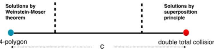
Let I = (H(A), H(B)) be the open interval. Denote

D_{= {c 2 I| Sc= H}−1_{(c) has a σ -invariant connected component S}σ_c} G_{= {c 2 I| Sc= H}−1_{(c) possesses a reduced simple choreography on it}} Then

µ(G ) = µ(D)

The theory of symmetric holomorphic sphere is developed in section 3.1-3.5. Then the proof of theorem E is carried out in theorem 3.6.1. As an application to the identical N-vortex problem, we can prove that

Consider the Hamiltonian

H_R2N(Z) = − 1

4π_{1i< jN}

∑

log |zi− zj|

2

Assume that N is even. Then there exist infinitely many non-trivial centred reduced relative choreographies.

The proof is summarized in theorem 3.7.2. The method is however applicable to other physical models, as is explained in theorem 3.7.1 and theorem 3.7.3.

We mention that we have also tried to apply the minimax method to find choreographies for the identical N-vortex problem. Unfortunately, we don’t know if the solution thus found is a relative equilibrium or not, hence according to our insistence on non-equilibrium, this minimax method might fail to meet our criteria of being suitable3_{. As a result we only report}

it in the appendix B in order not to diverge from the main points in the thesis.

1.5.3

An Uniform Bound Estimate for Symmetric Periodic Orbits

Finally In chapter 4, we study a uniform bound for Hamiltonians of N-vortex type. We have already seen that in general it is hopeless to have a uniform bound for periodic solutions of fixed period T . However, if we can have some symmetric constraints imposed on the orbit, it gives some extra control of the orbits. More precisely, define

M(z) = sup 1i< jN,t2[0,T]log |zi(t) − zj(t)| 2 _(1.39) ¯ M(T, N) = sup z2ΛT M(z) (1.40)

and ΛT stands for all the absolute centred T-choreographies of the N-vortex problem. we

prove the following theorem: Theorem G:

Let z(t) be a T-periodic solution of an N-vortex system where the Hamiltonian is of the form H(z) = −_4π1

∑

1i< jn

ΓiΓj|zi− zj|2

3_{Hilbert has posed his 19}th_{problem in the International Mathematical Congress that "Has not every} variational problem a solution, provided certain assumptions regarding the given boundary conditions are satisfied, and provided also that if need be that the notion of solution be suitably extended?”

1.5 Main Results 29 then

¯

M(T, N) < ∞

The proof is done in theorem 4.2.1 for orbits that are Italian symmetry, namely that z(t +T 2) =

−z(t). By similar argument the conclusion however holds for centred choreography too. Next we would like to study the bound for the action. To this end we study the re-parametrised Hamiltonian

G = exp (−

∏

1< jN|z i− zj|2)

We are interested in studying the trajectory space

M_{CH= {u : R ⇥ R \ T Z ! R}2N_{|8s 2 R,t 2 [0,T ],} ∂ u

∂ s+ J ∂ u

∂ t+ ∇G(u) = 0, E(u) < ∞ u(s, ) is an absolute centred choreography}

By using theorem G, one can prove a version of Gromov compactness for MCH. More

precisely, Theorem H: M_{CH is compact.}

This might serve as a starting step for the construction of Floer type theory of the N-vortex type Hamiltonian system.

Chapter 2

Periodic Orbits of the Positive N-Vortex

Problem

Abstract

In this chapter, we study the N-vortex problem in the plane with positive vorticities.

Γ˙z(t) = XH(z(t)) = J∇H(z(t)), ˙z = (z1, z2, ..., zN), zi= (xi, yi) 2 R2 (H1)

where the Hamiltonian is

H(z) = −_4π1

∑

1i< jN

ΓiΓjlog |zi− zj|2 (2.1)

After an investigation of some properties for normalized relative equilibria of the system, we use symplectic capacity theory to show that, there exist infinitely many normalized relative periodic orbits on a dense subset of all energy levels, which are neither fixed points nor relative equilibria. Let H0, H1, H2be defined as in chapter 1 we study the N-vortex

problem with positive vorticity. The main result is that: Theorem 2.0.1. If Γi> 0 (81  i  N), H2is dense in H0.

2.1

Sparseness of Relative Equilibria

Before we proceed to study NTNRPOs, we first need to have some preparation for properties of the normalized relative equilibria of H. =In this section, we study the normalized relative equilibria of H, with an emphasis on their energy levels.

2.1.1

Positive Vorticities

First note that the mutual distances between vortices in a normalized relative equilibrium configuration cannot be too small. More precisely:

Lemma 2.1.1. For Γi2 R+, there exists constant ε(Γ) which depends only on the vorticities

Γ = (Γ1, Γ2, ..ΓN), 1  i  N, s.t.

inf

z2Z1

1i< jN

|zi− zj|2> ε > 0

Remark 2.1.1. As the relative equilibria are rigid body motions, we have dropped the dependence of time of z to simplify the discussion.

This result first appears in the work of O’Neil [79] and has been reproved recently by Roberts [95] using a renormalisation argument, followed by a detailed discussion on Morse index of relative equilibria. We here give an alternative proof by the observation that for a relative equilibirum, the vorticity center of a given cluster also rotates uniformly.

Proof. : Denote

m(z) = inf

1i< jN|zi− zj| 2

Suppose to the contrary that zk_{is a sequence of relative equilibria whose mutual distances}

s.t. lim_k!∞m(zk_{) = 0. Then by consecutively passing to subsequence if necessary, we may}

suppose that there exists an sub-index set V ⇢ {1,2,..,N} s.t. zk

i ! z⇤, 8i 2 V . Denote zVas

the vector of vortices with index in V. The Hamiltonian could be separated into two parts, the interactions between vortices in V and otherwise. Let H(z) = HV(z) + HVc(z), where

HV(z) = − 1 4π _{i< j}

∑

i, j2V ΓiΓjlog |zi− zj|2 (2.2) HVc(z) = − 1 4π

∑

_{i< j} (i, j) /2V ⇥V ΓiΓjlog |zi− zj|2 (2.3)