MÉMOIRE PRÉSENTÉ À
L'UNIVERSITÉ DU QUÉBEC À TROIS-RIVIÈRES
COMME EXIGENCE PARTIELLE
DE LA MAÎTRISE EN SCIENCES DE L'ENVIRONNEMENT
PAR
SAIDANEMRIAPPLICATION D'UN MODÈLE HYDROLOGIQUE CONCEPTUEL POUR L'ÉTUDE DES CRUES PRINTANIÈRES AU QUÉBEC
Université du Québec à Trois-Rivières
Service de la bibliothèque
Avertissement
L’auteur de ce mémoire ou de cette thèse a autorisé l’Université du Québec
à Trois-Rivières à diffuser, à des fins non lucratives, une copie de son
mémoire ou de sa thèse.
Cette diffusion n’entraîne pas une renonciation de la part de l’auteur à ses
droits de propriété intellectuelle, incluant le droit d’auteur, sur ce mémoire
ou cette thèse. Notamment, la reproduction ou la publication de la totalité
ou d’une partie importante de ce mémoire ou de cette thèse requiert son
autorisation.
À l'issue de ce travail, je tiens à remercier et à exprimer toute ma gratitude à mon directeur de maîtrise M. Christophe Kinnard, professeur du Département des sciences de l'environnement de l'Université du Québec à Trois-Rivières, de m'avoir donné l'opportunité, pour la confiance qu'il m'a accordée, pour sa disponibilité, son efficacité et l'effort fourni.
Je tiens aussi à remercier les membres du jury qui ont accepté d'évaluer mon travail: MM. Ali Assani et Stéphane Campeau, professeurs du Département des sciences de l'environnement de l'Université du Québec à Trois-Rivières.
Je remercie également chaleureusement mes collègues et amis du Laboratoire en environnement des régions froides (GLACIOLAB), Lisane Arsenault, Okan Aygun, Hadi Mohammadzadeh Khani, Olivier Larouche, Arthur de Grandpré, Matthieu Loyer, Vasana Dharmadasa pour leur écoute, encouragement et tous les agréables moments qu'on a vécu ensemble.
À mes chers parents qui ont toujours été à mes côtés, à mon cher mari que rien n'aurait été possible sans vous et je vous en suis très reconnaissante!
La problématique envisagée par les hydrologues, dans un contexte de prédominance de neige en hiver et de fonte rapide au printemps, est d'avoir une estimation réaliste du couvert nival et de comprendre la complexité des facteurs qui contrôlent la génération des crues printanières. La modélisation hydrologique et de l'accumulation et la fonte de la neige par des modèles hydrologiques à différentes complexités constituent un outil pour la prévision opérationnelle des crues et la simulation du manteau nival. Dans cette étude, nous chercherons à améliorer la calibration d'un modèle hydrologique conceptuel couplé avec un module de fonte de la neige par l'ajout des données observées de l'équivalent en eau de la neige (ÉEN) dans le but d'obtenir une simulation réaliste du couvert nival dans une première étape. Dans une deuxième étape, nous avons essayé de comprendre la variabilité interannuelle de la magnitude et de la date d'occurrence des pics de crues printanières et de répondre à la question: est-ce que cette variabilité dépend principalement du stock de neige maximal accumulé, et quel est l'effet de la quantité et de l'intensité de la pluie durant la période de fonte sur le pic de crue? La performance de deux modèles, GR4J et Cemaneige, a été testée tout d'abord sur 12 bassins à régime hydrologique naturel et la calibration a été réalisée selon quatre stratégies. Un calage classique par rapport aux débits mesurés a été réalisé en premier temps en utilisant une méthode d'optimisation locale et ensuite avec un algorithme global (SCE-UA) dans la deuxième méthode. La troisième méthode consiste à calibrer indépendamment le module de neige avec l'équivalent en eau (ÉEN) observé aux stations du réseau nivométrique et l'introduire par la suite dans le modèle hydrologique. Une calibration multi-objectif a été entreprise par la suite, où les paramètres du modèle ont été calés par rapport à l'ÉEN et le débit observé, en utilisant un algorithme d'optimisation multi-objectif AMALGAM. Une amélioration de la simulation du couvert nival et du débit par la méthode multi-objectif a été démontrée. Les jeux de paramètres équifinaux ont montré une interaction et une compensation entre les paramètres qui constituent une grande source d'équifinalité. Sur une période de pré-conditionnement des crues, les facteurs liés à la fonte de neige, la pluie liquide enregistrée et l'humidité de sol ont été calculés et par la suite leurs capacités à expliquer les caractéristiques des pics printaniers (magnitude et date d'occurrence) ont été évaluées par une régression linéaire multiple. Nos résultats de régression linéaire démontrent que la variabilité interannuelle de la magnitude de crues printanières à travers les douze bassins dépend des facteurs suivants en ordre d'importance : l'intensité de fonte (moyenne et maximale), le total de la fonte, le total de la pluie, le pic de l'équivalent en eau (ÉEN) et l'humidité du sol. La pluie pré-crue contrôle principalement la variabilité interannuelle du pic de crue dans les bassins forestiers situés plus au nord avec un régime nival. Cependant, l'importance du stock de neige accumulé en hiver contrôle davantage cette variabilité dans les bassins du sud, plus agricoles et à régime davantage pluvio-nival. La date d'occurrence est plutôt expliquée par la pluie pré-crue. Mots-clés: crues printanières, variabilité interannuelle, magnitude, date d'occurrence, calibration, modèles hydrologiques conceptuels, ÉEN, incertitude des paramètres, changements climatiques.
REMERCIEMENTS ... ii
RÉsuMÉ...
iii CHAPITRE 1INTRODUCTION ... 1 1.1 Mise en contexte ... . 1.2 Problématique ... ... ... ... ... ... ... ... ... ... 2 1.3 Objectifs.. ... ... ... ... ... ... ... ... ... .... ... 2 CHAPITRE II
COMPARING CALIBRATION STRATEGIES OF A CONCEPTUAL SNOW HYDROLOGY MODEL AND THEIR IMPACT ON MODEL PERFORMANCE AND PARAMETER IDENTIFIABILITY... 4 Abstract ... 5 Introduction... 6 Data and methods... Il Study site and data ... ... ... ... ... ... ... ... ... Il Models ... 12 Calibration strategies ... 14 Parameters equifinality . ... ... ... ... .... ... ... ... ... 15 Parameter sensitivity analysis.... ... .... ... ... ... ... ... ... 15 Climate sensitivity ... 16 Results ... 16 Models performance... 16 Parameters interaction ... 18 Identifiability analysis of GR4J-Cemaneige parameters ... 19 Equifinality under changing climate... 20 Discussion and conclusion... 21
SWE simulation ... ... ... ... ... ... ... ... .... ... ... 21 Equifinalty and model structure uncertainty... 23 Conclusion ... ... ... ... ... ... ... ... ... .... ... ... 26
List of tables... 28
List of figures... 31
References... 44
CHAPITRE III MECHANISMS OF SPRING FRESHET GENERATION IN SOUTHERN QUEBEC, CANADA ... 51
Abstract ... 52
Introduction ... ... ... ... ... ... ... ... ... ... ... ... 53
Study Area and Data ... ... ... ... ... ... 56
Methodology ... ... ... ... ... ... ... .... ... ... ... ... 59
Spring flood identification ... ... ... ... ... ... ... 59
Antecedent factors and statistical analysis of spring freshet peak... 60
Results... 61
Inter-annual and spatial variability of peak streamflow and its date of occurrence... 61
Contribution of melt and rain to flood volumes.... ... ... ... 62
Correlation between antecedent factors and spring flow peak and timing... 63
Multivariate regression ... ... ... ... ... ... ... ... 64
Uncertainties of simulated predictors ... 66
Extremes events as simulated by conceptual model... 68
Discussion and conclusion... 72
List of tables.... ... ... ... ... ... ... ... ... ... ... ... ... 77 List of figures... 86 References .... ... ... ... ... ... ... ... ... ... 95 CHAPITRE IV CONCLUSION GÉNÉRALE ... 99 RÉFÉRENCES BIBLIOGRAPHIQUES... 102
INTRODUCTION
t.
t
Mise en contexteL'hydrologie dans les pays nordiques comme le Canada se distingue par de longs hivers dominés par la neige et une fonte printanière rapide. Cette fonte saisonnière fournit plus de 80 % du ruissellement annuel dans les prairies canadiennes (Buttle, 2016). Au Québec la quantité de neige accumulée est très importante avec un maximum annuel moyen de 200 à 300 mm d'équivalent en eau (Brown, 2010). Dans le nord du Québec, l'accumulation de neige commence en octobre et continue jusqu'au mois de mai tandis qu'au sud la neige commence à s'accumuler en novembre jusqu'à la fonte en mars-avril (Buttle et al., 2016). Le régime de ruissellement est fortement influencé par l'écoulement de la fonte des neiges au printemps et le débit le plus élevé est typiquement mesuré pendant cette période, le régime hydrologique des rivières se caractérise alors par une principale crue printanière (Adamowski, 2000), une crue secondaire faible liée aux précipitations en automne, une période de faible débit en hiver résultant de la chute de précipitations sous forme de neige et une autre période de faible débit en été suite à la diminution des précipitations liquides et solides (Assani et al., 2012). La relation entre le volume de neige et les débits de crues printanières a constitué le sujet de recherche de plusieurs études dans le but de prédire les crues, étudier les facteurs qui les préconditionnent et estimer la contribution du volume de la fonte à ces débits. Pour les gestionnaires des ressources en eau, une connaissance précise de l'équivalent en eau des neiges (ÉEN) des manteaux nival dans les derniers jours d'hiver est très importante pour la prévision du moment et du volume de crue printanière (Turcotte et al., 2010). L'état hydrique du sol ainsi que la contribution de la pluie aux crues peuvent influencer l'estimation de la vraie contribution nivale à ces crues. La modélisation de l'accumulation et la fonte de la neige par des modèles de neige et hydrologiques à différentes complexités constituent un outil pour la prévision opérationnelle des crues.
Une simulation réaliste du manteau nival présent sur le bassin suivi d'une bonne calibration et validation de ces modèles hydrologiques peut fournir une estimation réaliste de la contribution respective de la pluie et de la fonte de la neige aux débits en réponse aux conditions hydro-climatiques au moment des crues.
1.2 Problématique
Les crues printanières causent parfois des inondations qui provoquent d'importants dégâts matériels. Une meilleure compréhension des conditions hydroclimatiques causant les crues est souhaitable et représente la première étape vers le développement de méthodes de prévision des crues à l'échelle opérationnelle (jours) et saisonnière (mois). L'étude des facteurs préconditionnant les crues est difficile au Québec en raison du peu de données hydrométéorologiques disponibles. Quoique des données fiables de précipitation et températures existent, le bilan d'humidité du sol et la quantité de neige au sol, deux facteurs influençant fortement les crues, ne sont pas mesurés de façon routinière. L'utilisation de modèles hydrologiques peut ainsi contribuer à améliorer notre compréhension des facteurs qui pré conditionnent les crues printanières. La calibration classique des paramètres des modèles de neige se fait typiquement par rapport aux débits avec des critères de performance globale calculés à partir des débits observés et simulés (Troin et al., 2015; Valéry et al., 2014a, 2014b). Sauf que dans un bassin dominé par la fonte des neiges, une bonne simulation de débit à la sortie ne garantit pas toujours une bonne représentation des processus de neige.
1.3 Objectifs
L'objectif principal de ce projet de recherche est d'étudier les caractéristiques hydrométéorologiques des crues printanières au Québec à l'aide d'un modèle hydrologique simplifié (modèle GR4J) et un modèle de fonte à base de degré/jours (modèle Cemaneige) pour la compréhension des facteurs qui préconditionnent les crues printanières au Québec. Les objectifs spécifiques suivants ont été poursuivis:
1) Tester la performance d'un modèle pluie-neige-débit pour 12 bassins au Québec. La question principale qui sous-tend cet objectif est la suivante: un modèle conceptuel et parcimonieux est-il adéquat pour bien simuler l'évolution du couvert nival et les débits de crues printanières? Le choix de la stratégie de calage/validation des deux modèles est le premier défi à relever dans cette étape, qui comprend le choix de la fonction objectif et d'un algorithme d'optimisation permettant d'utiliser simultanément les relevés de neige et les débits observés. Nos principales hypothèses qui ont été testées pour cette partie sont 1) la calibration multi-objectif (débit et neige) améliore la simulation des débits et du manteau nival et augmente la stabilité des paramètres (réduit l'équifinalité); 2) les paramètres hydrologiques seront spatialement plus homogènes, et mieux reliés aux caractéristiques du bassin lorsque les paramètres neige sont prescrits. Cet objectif va être l'objet du chapitre 1.
2) Identifier les variables, telles que simulées par le modèle GR4J-Cemaneige, qui préconditionnent les crues (apports de la fonte de la neige, pluies, bilan d'humidité du sol) et leurs variations spatiales. La question qui sous-tend cet objectif est la suivante: quelle est la contribution respective de la pluie, de la fonte des neiges et de l'état hydrique du sol aux pics de crues printanières? Les hypothèses qui ont été testées sont 1) la contribution de la pluie au volume de crue printanière varie entre les bassins, selon la latitude; 2) la variabilité interannuelle de la magnitude du pic de crue printanière ainsi que sa date d'occurrence dépend principalement du stock de neige accumulé, et secondairement de la quantité de pluie durant la période de fonte; 3) plus le stock de neige est important, plus longue sera la fonte et le niveau des rivières montera plus haut; 4) plus il y a de pluie durant la fonte, plus le niveau montera. Les résultats de cette deuxième partie seront l'objet du chapitre II.
COMP ARING CALIBRATION STRATEGIES OF A CONCEPTUAL SNOW
HYDROLOGY MODEL AND THEIR IMPACT ON MODEL PERFORMANCE
AND P ARAMETER IDENTIFIABILITY
Article en attente de soumission au journal scientifique Journal of Hydrology
Saida Nernri l, Christophe Kinnard 1
1 Département des Sciences de l'environnement, Université du Québec à Trois-Rivières, C. P. 500, Trois-Rivières, Québec, G9A 5H7 Canada
Corresponding author: Christophe Kinnard
Abstract
Having a realistic estimation of snow coyer by conceptual hydrological models continues to challenge hydrologists. The calibration of the free parameters is an unavoidable step in modeling and the uncertainties resulting from the use of this optimal set remains a source of concem, especially in fore casting applications and climate changes impact assessments. The objective of this study is to improve the calibration of the conceptual hydrological model GR4J coupled with the snowmelt model Cemaneige, in order to obtain a more realistic simulation of the snow water equivalent (SWE) and to reduce the uncertainty of the free parameters. The performance of the two models was tested over twelve snow-dominated basins in southem Quebec, Canada. Four calibration strategies were adopted and compared. In the first two strategies, the parameters were calibrated against observed streamflow only using a local and a global algorithm. In the third and fourth strategies the calibration of snow and hydrological parameters was performed against observed discharge and snow water equivalent (SWE) measured at snow survey points, first separately, and then with a multi-objective approach using the AMALGAM algorithm. An ensemble of equifinal parameters was used to compare the capacity of the global and multi-objective algorithms to improve the parameters identifiability, and to quantify their uncertainties in the detection of climate change impact on spring peak streamflow. Results show that the inclusion of snow observations using the multi-objective approach improved the simulation of SWE and the identifiability of the parameters. The large number of equifinal parameters found during calibration shows the importance of structure no-identifiability in the coupled GR4J-Cemaneige mode!. The uncertainty induced by using the best numerical optimal solution rather than equifinal parameters giving a similar performance, for detecting
changes in maximum spring streamflow in response to climate warming in
snow-dominated basins, is not negligible.
Keywords: conceptual hydrologic model; calibration; SWE; structural uncertainty; equifinality; climate change.
Introduction
In cold regions, the accumulation of snow in winter and the rapid melting during the warm period is the main source of the high spring streamflow. In these areas, a good estimation of the amount of snow present in a basin before melting is the starting point of any floods forecasting and essential to understand the interannual variability of the magnitude and the timing of snow melting. In the Canadian province of Quebec,
the amount of accumulated snow is considerable, with a mean annual maximum of 200 to 300 mm in terms of water equivalent (Brown, 2010). Melting of this snow in the spring represents an important source of freshwater which shapes the ecology of the region as well as hydropower generation capacity (Brown, 2010). In Québec, a network of snow survey measurement sites was installed by the Ministry of Environment and Fight Against Climate Change (MELCC) since 1928 for operational purposes to monitor snow cover depth and snow water equivalent (SWE) (Poirier et al., 2014). Remote sensing data (passive and active microwaves) has also been widely used for estimating SWE but problems remain in forested areas and regions with thick snow cover, as weIl as in steep mountain terrain (Brown, 2010; Turcotte et al., 2007).
Consequently, hydrological models of different complexities have been mainly used by hydrologists to simulate the accumulation and melting of snow and to estimate streamflow for operational purposes (Turcotte et al., 2010). Several rainfall-runoff models have shown a great ability to simulate runoff, but in a snow-dominated basin, a good streamflow simulation does not al ways guarantee a good representation of the snow processes (Udnres et al., 2007). Accurate simulations of both river discharge and snow cover are desirable if these models are to be used to project potential impacts of climate change on snow hydrology.
Model calibration is necessary to estimate the free parameters in conceptual models, and many questions still arise about how the uncertainties in the calibrated parameters impact streamflow forecasts as weIl as model-based climate change projections. In its beginning, the calibration problem was a numerical problem which often led to miscalibration, as described by Andréassian et al. (2012), due to the high-dimensional response surfaces of the parameters and the failure of algorithms to locate
global mathematical optima without being trapped by local ones (Moradkhani et al.,
2009). Therefore, several optimization algorithms (local, global) were developed during the last decades, with the objective to improve both the search algorithms and the evaluation criteria used during calibration and validation. Several important reviews in the li te rature have illustrated and compared the optimization methods developed and used by hydrologists (Duan et al., 1992; Efstratiadis et al., 2010; Gupta et al., 2006; Gupta et al., 2003b; Moradkhani et al., 2009). The Shuffled Complex Evolution -University of Arizona (SCE-UA) algorithm elaborated by Duan et al. (1992) is often considered the most efficient for the calibration of conceptual and global hydrological models because of its ability to find global optima (Arsenault et al., 2013). Despite the
development of sophisticated automatic algorithms and calibration methods,
the uncertainties related to calibrated parameters has persisted while new uncertainty problems have been revealed (Blasone, 2007). The major issue is the multiplicity of optimal parameters, whereas several sets of parameters give the same performance, and this remains at the heart of aIl studies on the robustness of hydrological models.
The concept of a single optimal set has been gradually replaced to accept that a group of parameter sets can give equally satisfying simulations, a concept called 'equifinality' by Beven (2006). Nurnerous hydrological studies have focused on quantifying equifinality and its impact on simulations (Arsenault, 2015; Arsenault et al., 2014; Beven, 2006; Beven et al., 2001; Foulon et al., 2018). This multiplicity is also explained by the dependence between the optimized parameter values and the climatic conditions of the calibration period, which was highlighted by several authors using a multi-calibration approach on climatically contrasted sub-periods (i.e. periods of similar climatic conditions) (Blasone, 2007; Brigode et al., 2013; Coron et al., 2014; Coron et al., 2012; Merz et al., 20 Il; Perrin, 2000; Seiller et al., 2012; Vos et al., 2010). These studies also demonstrate the problem of the temporal transferability of parameters, i.e. when they are calibrated over a period and transferred to another period with different climatic conditions. Gupta et al. (1998) also explained this multiplicity of optimal sets by the natural multi-objectivity of the parameters that are related to the calibration objective function. In the context of snow-dominated basins, the parameters of the snow models are most often calibrated simultaneously with the hydrological parameters against
observed discharge, without taking into account any infonnation about snow (e.g. Troin et al., 2015; Valéry et al., 2014a, 2014b). Hence in addition to the aforementioned calibration uncertainties, the representativity of key processes such as snow melting represents another important issue in these basins, especially wh en using these models for climate change studies. A multi-objective approach was recommended by hydrologists to replace this classical calibration method to improve the simulation of all processes and to reduce uncertainties in the free parameters (Efstratiadis et al., 2010; Gupta et al., 1998). This is typically carried out using evolutionary algorithms that se arch for acceptable trade-offs between objective functions and leads to a feasible vector called 'Pareto optima lit y' (Yapo et al., 1998). Several studies have already shown the utility of including snow observations in the calibration of different models within a multi-objective approach to improve the simulation of SWE (Duethmann et al., 2014; Fenicia et al., 2007; Finger et al., 2011; Madsen, 2003; Parajka et al., 2008; Parajka et al., 2007; Turcotte et al., 2003). Snow coyer area (SCA) estimated by satellite sensors such as MODIS and Landsat are among the snow observations used to calibrate and validate snowmelt models (Duethmann et al., 2014; Finger et al., 2011; Parajka et al., 2008). In Quebec, Roy et al. (2010) incorporated snow-covered area derived from remote sensing to improve spring streamflow simulation with the Hydrotel model. Turcotte et al. (2007) used snow survey observations (density and SWE) to calibrate the Hydrotel model at each snow survey station.
Lumped or semi-distributed models are among the most used models to assess climate change impacts on water resources (Wilby, 2005). Uncertainties in climatic scenarios and downscaling techniques are known to cause significant uncertainties in hydrological impact assessments (e.g. Wilby, 2005). Several recent studies have also focused on the uncertainties induced by hydrological modeling, i.e. those resulting from structural and parameterization errors. Sorne of these studies attempted to rank these uncertainties, but there is no agreement yet on the ranking of hydrological and climatic errors, and between hydrological uncertainties themselves, i.e. structural errors and parameters equifinality (Bennett et al., 2012; Kay et al., 2009; Seiller et al., 2014; Teng et al., 2011; Wilby, 2005; Wilby et al., 2006). Uncertainty arising from the model
structure is typically evaluated by using multiple hydrological models having different structures, and so different representations of hydrology processes, to see the spread of future hydrological projections for the same c1imatic scenario (e.g. Chen et al., 20 Il; Jiang et al., 2007; Poulin et al., 2011; SeilIer et al., 2014). Seiller et al. (2014) compared the uncertainties arising from c1imatic variability and the choice between twenty lumped hydrological models and seven snow models, and found that the uncertainty in simulated streamflow arising from models structures was less important than uncertainties in c1imate scenarios. Wilby et al. (2006) ranked parameter uncertainty as the third most important source, behind the choice of GCM and downscaling technique. Chen et al. (20 Il) ranked the structural uncertainty as the fourth and parameters uncertainties as the fifth most important, behind climatic uncertainties, for a Canadian catchment. In aIl these studies, structural and parameterization uncertainties were evaluated jointly.
The impacts of parameters non-uniqueness on hydrological projections have been addressed by generating equifinal parameter sets using different methods and running the model using this ensemble. Wilby (2005) studied the uncertainties caused by conceptual model structure, parameter equifinality and the choice of calibration period (wet, dry). He used two different model structures and 100 equifinal parameter sets sampled by Monte Carlo sampling and two emission scenarios, and found that the uncertainty on projected monthly mean river flows due to parameter equifinality was higher in winter than summer and comparable to those related to emission scenarios.
Kay et al. (2009) used two different versions of a conceptual model and a jackknifing method to generate parameter sets and found that the uncertainty related to climate modeling was higher th an that arising from hydrological modeling. In a snow-dominated basin of southem Québec, Poulin et al. (20 Il) used two hydrological model versions and equifinal parameter sets obtained by multiple calibrations with the SCE-UA algorithm,
and found that model structural uncertainties are more important th an parameter uncertainty due to equifinality under c1imate change, insisting that this structural uncertainty should be considered in hydrological impact assessment studies. Bennett et al. (2012) used 25 Pareto solution sets obtained by the multi-objective algorithm MOCOM and found that hydrological parameter uncertainty was less than the uncertainties related to GCMs and emissions scenarios for three snow-dominated basins
in British-Colombia, Canada. Ficklin et al. (2014) examined the effects of parameter equifinalty on hydrology in the SWAT model using outputs from five GCMs and showed that equifinal sets can lead to statistically significant differences in projected streamflow, snowmelt rates and timing under climate change. Hence the use of a single parameter set to project future streamflow under climate change with the SW AT model was deemed to be not robust in snow-dominated basins. Brigode et al. (2013) tested two models, GR4J and TOPMODEL, on 89 catchments in France to study the uncertainties related to parameter instability (dependence to calibration climate conditions) and parameter equifinality in a climate change context. They used the GLUE method to identify 2000 posterior parameters sets and found that the uncertainty arising from the temporal transferability of parameters was higher than that from equifinality. Her et al. (2016) studied the uncertainties related to climate models and hydrological parameter equifinality under climate change using the GLUE method and different thresholds to identify behavioral parameter sets. They showed that parameter uncertainty depends on the choice of hydrologic indicator and has a greater influence on soil moisture and groundwater projections than climate model uncertainty. Foulon et al. (2018) assessed the impact of equifinality and the choice of objective function on several hydrological indices, including SWE and maximum winter peak flows. Their study was conducted over 10 basins in Québec with the Hydrotel model, using 250 equifinal sets and different objective functions computed on streamflow. They found that the choice of objective function was most important for SWE, while parameter equifinality was a more important source of uncertainty for the other hydrologic indices. The authors insisted that equifinality should be systematically taken into account in future work. Most of the aformentionned studies compared the sources of uncertainty and demonstrated that uncertainties induced by hydrological models are less important than climate models, but nonetheless suggested that they should be evaluated when performing climate change impact assessments.
The mam question of interest in this study is whether simple conceptual hydrological models are capable to adequately simulate runoff as weil as snow cover in snow-dominated basins and how stable are the optimized parameters. Therefore, the
main objective of this study is to improve the simulation of snowpack by a parsimonious hydrological model, GR4J (Perrin et al., 2003), coupled to the snow model Cemaneige (Valéry, 2010) by considering available SWE observations from the Quebec permanent snow measurement network in the model calibration. We further investigate different calibration strategies, by (i) comparing the respective performance of a local, global and multi-objective algorithm for twelve snow-dominated basins in Québec, and (ii) comparing how the calibration strategy improves the parameters identifiability. Finally, we test how the uncertainty related to parameter equifinality impacts the assessment of streamflow sensitivity to climate change. The goal is not to perform a thorough, scenario-based climate change impact assessment nor to compare the different sources of uncertainties, but rather to focus on the impacts of choosing either a mathematically-optimal parameter set versus several equifinal parameter sets on the detection of a climate changing signal in selected streamflow signatures.
Data and methods
Study site and data
Twelve tributary basins of the St. Lawrence River in Quebec were selected in this study (Fig. 1). The choice was based on the length of observed discharge data (> 20 years), the natural character of the hydrological regime of the ri vers and,
especially, the availability of snow measurement points inside or close to the studied
basin. The area of the basins varies between 367 and 4504 km2 (Table 1). They are located in four homogeneous hydrological regions, namely (i) the St. Lawrence northwest region (Batiscan, Bras du Nord, Matawin) on the north shore and characterized by a continental climate; (ii) the St. Lawrence southwest region (Nicolet, L'Acadie) characterized by a mixed maritime and continental climate; (iii) the St. Lawrence southeast region (York, Beaurivage, Bécancour, Famine, Etchemin,
Ouelle) characterized by a mix of maritime and continental climate, and (iv) the St. Lawrence northeast (Godbout) characterized by a maritime climate (Assani et al.,
Daily historical discharge data measured at the basin outlets were extracted from the website of the Quebec Center of Water Expertise (CEHQ) (www.cehq.qc.ca). The climatic data used were extracted from the daily climate grids developed by the Atmospheric Environment Information Service (SIMAT) in collaboration with the CEHQ (Bergeron, 2015). The total daily precipitation (solid and liquid), minimum and maximum temperature at each grid point are estimated by spatial interpolation (kriging) using stations managed by the Quebec Climate Monitoring Program (Programme de surveillance du climat du Québec: PSC) and stations operated by the national hydropower company Hydro-Québec. The interpolated climate grids are considered to be of good quality in the southem part of Quebec given the high density of stations in this region. Continuous data are available for the period from 1961 to 2015 (Bergeron, 2015). The snow observations come from the permanent snow survey network maintained by the Ministry of Environment and Fight Against Climate Change (MELCC). Survey sites are located in forested areas where the depth and density of snow is measured every two weeks during the winter and spring seasons. Each SWE observation at a given survey site represents the average of ten manual measurements made with a snow tube along a 100 rn-long transect. The historical measurements of 12 survey sites located in or very close to the selected basins were used. The snow survey sites and the characteristics of the basins are shown in Table 1.
Models
The GR4J (modèle du Génie Rural à 4 paramètres Journalier) hydrological conceptual model (Perrin et al., 2003) and the Cemaneige snow model (Valéry, 2010) were chosen in this study to simulate the snow coyer and hydrology of the basins.
In the GR4J model, hydrological processes in the basin have been simplified into two interconnected reservoirs. The production function, which determines the amount of water in the basin, is represented by a soil reservoir with a maximum capacity xl (mm) which is the first parameter to be calibrated. The transfer function, which determines the transfer of water in the water basin, is represented by a routing reservoir which receives the quantity released by the production function and calculates a discharge linked to its
level of filling and its maXImum retention capacity at 1-day, x3, which is a free parameter. Edijtano (1991) added a function to simulate water transit time to the routing reservoir by a unit hydrograph to improve the simulation of flood peaks in which 90% of the water released by the production store is routed by a unit hydrograph to the routing reservoir, while the remaining 10% contributes directly to flow and is routed only by a unit hydrograph. The base of the unit hydrograph, x4 (mm/day), is a free parameter. The model was previously found to give poor simulations in basins with intermittent flow regimes. For this reason, Nascimento (1995) added a groundwater exchange function to the routing reservoir and to the direct flow compone nt which improved runoff simulations. This exchange coefficient, x2 (mm/day), can be negative (losses to the aquifer) or positive (inflow from the aquifers) and this is why the model no longer considers the basin as a conservative water balance system but rather as an open system (Perrin, 2000; Perrin et al., 2003; Perrin et al., 2007). The version of GR41 from Perrin (2000) is used in this study.
Developed by Valéry (2010), the Cemaneige module with two free parameters simulates snow accumulation an melt in the basin with one snow reservoir for each of five altitude bands. The two internaI states of the snowpack simulated are the snow storage (snow water equivalent) and the thermal state. The snow storage is initially zero and increases at each time step after adding the solid fraction of the precipitation.
The thermal state of the snowpack (OC) determines the onset of melting and is calculated by a weighting coefficient, x5 (dimensionless), which is a free parameter of the model to be calibrated and varies between 0 and 1. A value of 1 describes a maximum thermal inertia of the snow compared to air temperature. After the calculation of the snow storage and its thermal state, the model calculates the potential melt which represents the maximum amount of snow that can melt using the degree-day method. The degree-day factor, x6 (mm °C l), controls the potential melt and is a free parame ter to be calibrated. Six parameters must then be calibrated for the coupled GR41-Cemaneige model. Table 2 summarizes the description of these parameters. The ranges of hydrological model parameters are based on lite rature and previous studies (Perrin, 2000) while those for the Cemaneige model were chosen based on the work of Valéry (2010).
Calibration strategies
In the calibration strategy, the choice of optimization algorithm and objective functions have a great influence on the identification of the parameters and their uncertainty, in addition to the structure of the model and the quality of the input data. The objective of improving the snow coyer simulation by the GR4J -Cemaneige model and the identifiability of the parameters led us to consider four calibration strategies in which three algorithms (local, global and multi-objective) were used: for the first two strategies, the calibration of the six GR4J-Cemaneige model parameters was done simultaneously using the observed discharge, with respectively a local 'pas-à-pas' approach (strategy 1: 'LOCAL') and the global SCE-UA algorithm (strategy 2: 'SCE-FLOW'). The local 'pas-à-pas' (step-by-step) optimization algorithm was used for the development and improvement of the two models by researchers at Cemagref, France (Perrin, 2000). The global automatic algorithm Shuffled Complex Evolution (SCE-UA) developed by Duan et al. (1992) is considered the most efficient by hydrologists. The SWE simulated by these two strategies was then compared with the SWE observed at the nivometric survey points in, or closest to, the selected basins, for the elevation band closest to the elevation of the snow survey point. In the third strategy, 'SCE_INDEP', the four hydrological model parameters and the two snow parameters were calibrated separately. The two snow parameters were calibrated with the observed SWE and prescribed subsequently as fixed parameters in the coupled GR4J-Cemaneige model. The four hydrological parameters were next calibrated with the observed discharge by the global SCE-UA algorithm. The fourth and final multi-objective strategy, 'MULTI', was finally applied in which the six model parameters were calibrated simultaneously with the observed SWE and discharge using the multi-objective optimization algorithm AMALGAM (Vrugt et al., 2007). The split-sample test calibration method (Klemes, 1986) was used to separate the observation record into two equal length periods of calibration/validation (Table 1). The Nash-Sutcliffe (1970) efficiency criterion was used as the evaluation criterion and calculated from the observed and simulated discharge (Nash-Q) and from the SWE measured at surveys point and that simulated by the model for the corresponding elevation band (Nash-SWE):
Equation (1)
Equation (2)
where Qo and Qs are the observed and simulated discharge and SWEo and SWEs the observed and simulated snow water equivalent, respectively.
Parameters equifinality
Only the calibration methods SCE_FLOW and MULII were used in this step to study the interaction and the compensation between parameters. Iterations made by the algorithms during calibration until convergence were saved (more than 6000 for each basin). For the SCE-UA algorithm, the parameter sets yielding a Nash value within 1 %
of the optimal Nash value were considered equifinal. Similarly, for the multi-objective algorithm AMALGAM, the optimal point of the Pareto solution was chosen and aIl parameter sets around this point that gave the same optimal performance with a difference less than 1 % in the Nash criterion were retained.
Parameter sensitivity analysis
The dynamic identifiability analysis (DYNIA) method developed by (Wagener et al., 2003) was used after that to investigate the parame ter identifiability. This method consists in testing the identifiability of each parameter in a moving time window, set to 15 days here, by identifying the portion of the parameter range that give the best performance (Wagener et al., 2003). Finding a clear range of parameter values that give the best simulation means that this parameter is more identifiable in this time window, while the opposite means that aIl values within the range can give equaIly-best simulation in combination with other parameters. Time-varying sensitivity analysis (TVSA) (Pianosi et al., 2016; Reusser et al., 20 Il) is used also to investigate the most influential model parameters at each time step of the simulation and the consistency of
the parame ter role and its period of influence with the physical behavior of the basin (Pianosi et al., 2016; Reusser et al., 2011).
Climate sensitivity
The objective in this step is to assess how parameter equifinality and the choice of a single optimal parameter set versus several equifinal sets impact the characterisation of streamflow sensitivity to climate change. We focus here on the sensitivity of the average annual springtime peak streamflow (Qmaxsp) and its timing (QmaxspT) to a +2 oC increase in mean air temperature. Only the equifinal sets obtained by the third calibration strategy, the most used in lite rature , was considered III this part (SCE-FLOW). The sensitivity measures used (~Qmaxsp), is the percent difference between the mean historical Qmaxsp obtained by the optimal set and that projected by the optimal set and equifinal sets under the warming scenario. The same approach was used for the peakflow timing (~QmaxspT, in days). The objective is to investigate the agreement between the equifinal and optimal sets about the evolution, i.e. the direction and magnitude of change, of an important hydrological indicator in southem Quebec which is the peak streamflow induced by snowmelt in spring.
Results
Models performance
For all calibration strategies, one global optimal parameter set was obtained, except for the multi-objective method MULTI where a vector of 'Pareto-optimal' parameter sets was obtained. The optimal point of the Pareto set that gives the best compromise between snow SWE and discharge was selected to compare with the performance of the other calibration strategies. Boxplots in Fig. 2 show the model performance for the 12 selected basins and the four calibration methods for both the calibration and validation periods. With the first method LOCAL (Fig. 2aI) the model shows a good performance in discharge simulation with a median Nash-Q value of 84%
in calibration and 80% in validation but a comparatively poor performance in SWE simulation: the median Nash-SWE value is around 40% during calibration and increases to 58% in validation, but the spread of the distribution is higher (Fig. 2a2). The calibration results with the global algorithm SCE_FLOW also show a good streamflow simulation with a median Nash-Q value of 82% in calibration, similar to the first method, but with an improvement in validation with the median Nash-Q value increasing to 83% (Fig. 2bl). The SWE simulation is still weak with the SCE FLOW method but slightly improves nonetheless with the median Nash-SWE value increasing to 43% in calibration and 59% in validation (Fig. 2b2), but the spread of the distributions is still considerable and comparable to the first local method. In the third strategy SCE_INDEP, the two Cemaneige parameters were calibrated separately against the
observed SWE, which improved significantly the Nash-SWE in calibration with a
median value of 58%. This significant improvement in the Nash-SWE criterion is however accompanied by a degradation of the flow simulation, with the median Nash-Q value decreasing to 80% in calibration and 76% in validation, which means that the introduction of two fixed snow parameters in the GR4J-Cemaneige model led to an over-adjustment on the SWE and a degradation in the streamflow simulation (Fig. 2c). The multi-objective strategy in which the Nash-SWE and Nash-Q are simultaneously optimized (Fig. 2d) improved the simulation of the SWE, with 75% of the basins having a Nash-SWE greater than 50% in calibration and greater th an 40% in validation, without significantly degrading streamflow simulations (Fig.2dl). The simulation of SWE is
hence significantly improved for the two methods SCE_INDEP and MULTI in which
the snow observations are taken into account (Fig. 2c-d), but the method SCE _ INDEP degrades the simulation of discharge. The best simulation of SWE in both calibration and validation without significant streamflow degradation is obtained by the MDL TI method, for which the model efficiency ranged between 31 and 84% for the 12 basins (Fig. 3). The best SWE simulations were obtained for the Famine, Beaurivage, Ouelle, Bécancour, and Bras de Nord basins, with a Nash-SWE criterion above 65% while the poorest simulation were obtained for the Matawin and Acadie basins. The poor simulation in these two basins may be due to the survey sites being less representative of the basin, which is an obvious limitation of using point observations to constrain the
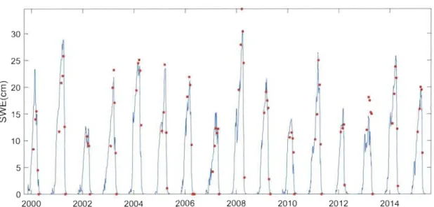
snow mode!. Fig. 4 shows an example of SWE simulation for the Bécancour catchment with the MDL TI method.
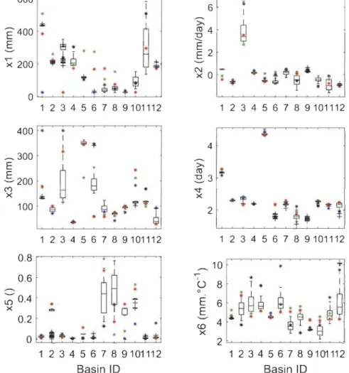
Parameters interaction
The distribution of the optimal parameters obtained for the 12 basins is different between the calibration strategies, except for the parameter x4 (base of the unit hydrograph) and x2 (water table exchange) which are more similar (Fig. 5). The choice of the calibration method does not seem to have a clear impact on the distribution of the parameters between the basins. For the third method SCE_INDEP,
where the calibration of the Cemaneige parameters is do ne separately on the SWE observations, the degree-day factor x6 which determines potential snowmelt is higher and more dispersed than for the other methods, while x5 (weighting coefficient of the thermal state), which determines the onset of melting, is minimized. Subsequently, the parameter xl (maximum capacity of the soil reservoir) approaches its lower limit in sorne basins while x3 (the routing reservoir capacity) approaches its upper limit. The optimal parameters obtained by each calibration strategy differ with each other for a given basin (Fig. 6). This shows that different optimal sets give the best simulation for each calibration method over the same period. The two parameters x2 and x4 are the only ones for which similar values are obtained from aU calibration strategies.
Equifinality was studied usmg two calibration methods, namely SCE _FLOW, which is the global algorithm most used in the literature and uses only observed discharge, and the method MULTI which gave the best performance (Fig. 3). The distributions of equifinal parameters obtained for the 12 basins by the procedure described in the methods section are presented in Fig. 7. The distributions for the SCE_FLOW method are narrow but with many extreme values, while the distributions for the multi-objective method are more homogeneous (Fig. 7). For the SCE _FLOW method the number of sets found is very high and variable between basins. Therefore, in order to converge mathematically with a very small change in the Nash value
«
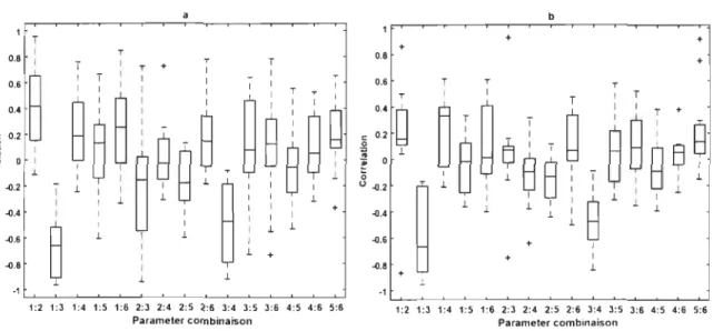
1 %),450 mm for basin 1 (Batiscan). Similar variability is seen for the other basins. The calibration with the multi-objective algorithm reduced the number of equifinal parameters sets and their dispersion (Fig. 7b). The MUL TI method also reduced the range, i.e. the difference between the maximum and minimum parameter value, but no significant reduction was found in the interquartile range compared to the SCE _FLOW method (Fig. 8). The correlation between the equifinal sets can explain this dispersion and multiplicity of parameters giving the same performance. A strong negative correlation is found between the two reservoir parameters, xl (the maximum soil reservoir capacity) and x3 (the routing reservoir capacity), with a median value of -0.7,
and between the two transfer parameters x3 and x4 (base time unit hydrograph) with a median value of -0.5 (Fig. 9). A positive correlation is also visible between x 1 and x2, which regulates the amount of water available in the basin, with a median value of 0.4 (Fig. 9a). This strong correlation shows the compensation between the parameters occurring during the optimization and the difficulty to converge toward an optimal set. This parameter correlation was significantly reduced when using the MUL TI method (Fig. 9b).
Identifiability analysis ofGR4J-Cemaneige parameters
The equifinality of parameters has led us to investigate more deeply the identifiability of the GR4J and Cemaneige parameters using the DYNIA and TVSA methods in order to understand the interaction of model parameters. The analysis was only performed in the Bécancour basin (ID#2) for the sake of brevity. The temporal identifiability of the six parameters of the GR4J-Cemaneige model found by the DYNIA method is shown in Fig. 10. In these graphs the color scale represents the frequency distribution of the parameters for a sample of the 10% best-performing simulations,
using the root-mean-squared error (rmse) as objective function. A parameter becomes more identifiable during periods when the frequency distribution is narrower. For the parameter xl, low values are more frequent before and during floods, while high values are more frequent after the floods. There is no c1ear part in this parameter space that is identifiable in the best-performing simulations, which indicates that different values of
this parameter give similar results in combination with the other parameters. Parameter x2 is a multiplicative parameter that regulates the volume of water in the basin: the more positive its value, the largest is the contribution of groundwater to the basin, while more negative values increase deep percolation losses. Fig. 10 shows that negative values are more frequent during low flow periods, indicating large water losses to deep aquifers simulated by the model. Conversely, high positive values ofx2 are more frequent during floods. This means that to simulate the high flows the model increases the supply from the water table while for the low flows the model increases the loss to the water table. The high sensitivity of x2 implies that the GR4J model first tries to use this parameter to adjust the water volume in the basin and then the other production parameter xl, which explains the difficulty of finding sensitive x 1 values conditioned on discharge. The parameter x3 (one-day capacity of the routing reservoir) is barely identifiable: high values are more frequent during and before the floods, and after the floods the models begins decreasing the its value but still the identifiability is unclear. The identifiability of the parameters x4 (base time of the unit hydrograph) and x5 (thermal coefficient of state of the snowpack) is low since very different values of these parameters give similar results in combination with the remaining parameters. Parameter x6 (degree-day factor) is somewhat identifiable during the melt period, with a value between 5 and 7 mm °C-1 giving the best simulation. Time-varying sensitivity analysis (TVSA) (Reusser et al., 20 Il) (Fig. Il) also shows that the parame ter x2 is the most influential, except during the spring pre-flood periods when the snow parameters x5 and x6 of the Cemaneige model become the most influential, whereas they have no influence on the rest of the period. This confirms that the behavior of the model is consistent with the physical behavior of the basin in the spring. The sensitivity of xl, x3, and x4 is not clear compared with x2, suggesting that the model tries to first use the x2 parameter value to adjust the flow and then uses the other parameters afterward.
Equifinality under changing climate
The final objective of this study was to assess how parameter equifinality and the choice of a single optimal vs. equifinal parameter set impact the characterisation of
streamflow sensitivity to c1imate change. The distribution of ~Qmaxsp values can thus be used to quantify the uncertainty in the sensitivity of springtime peak flow to warming which results from equifinality alone (Fig. 12) There is a general agreement between ail equifinal and the optimal sets that peak spring streamflow would decrease in the future in response to a +2 oC climate warming, as ail simulations display negative ~Qmaxsp
values. For ail basins the impact of a +2 oC c1imate warming on Qmaxsp can be detected using the optimal parameter set (red dot on Fig. 12) with a 99% confidence interval varying between ± 0.8% (basin 10) to ± 3.9% (basin 7), which is a rather low uncertainty. However, the distributions of sensitivities is not normal, and when we take into account ail the parameter sets inc1uding the numerous outliers, the range of reduction in Qmaxsp can be much greater, as much as 12% (-10 % to -22%) for basin 3 and 13 % (-4% to -17%) for basin Il. The difference of uncertainty between basins can be explained by the dispersion of equifinal parameters displayed in Fig. 7: basins with the most dispersed equifinal parameter distributions (ID# 1,3, Il) have the largest errors in their temperature sensitivities.
There is an agreement, except for basin 12, that peak springtime streamflow will occur earlier in response to a +2 oC temperature warming (Fig. 13). For basin #2 the peak streamflow could occur earlier by 2 to 10 days and for the two basins #7 and #8 the occurrence day could shift earlier by 3 to 9 days depending on the equifinal parameter set. For basin #12 (L'Acadie River), which is the southernmost basin studied (Fig. 1), the change in peakflow timing detected using the optimal parameter set is positive but the uncertainty due to equifinality, when considering outliers, is such that the direction of change in timing cannot be reliably detected for this basin.
Discussion and conclusion
SWE simulation
Having a good simulation of streamflow generated by snowmelt has always been an important objective of hydrologists during the development of snow models to be
used within hydrological models, and their performance has been generally assessed by their capacity to simulate observed streamflow, which was the case for the development of the Cemaneige model (Valéry, 2010). The objective is most often to obtain the best efficiency criteria between observed and simulated streamflow, which does not always guarantee that other processes such as snowmelt are properly simulated by conceptual models. The contribution of this study was mainly to test the use of snow survey points to improve the calibration of the conceptual models GR4J and Cemaneige while avoiding the difficulties related to snow cover satellites products. Four calibration strategies have been tested for the simulation of discharge and SWE using a local, global and multi-objective algorithrn. After comparing results obtained by the different methods, it appears that overall the calibration against observed discharge in the first two methods yielded good streamflow simulations but poor simulations of SWE. The global algorithrn SCE-UA yielded a better streamflow simulation in validation that the local algorithm, confirming previously reported results about the ability of global algorithrns and specifically the SCE-UA to find global optimal parameters, unlike the local algorithrns that depend on initial sets (Efstratiadis et al., 2010). Despite this
mathematical power of the SCE-UA algorithrn in fin ding the global optima,
its performance in simulating SWE was very similar to the local algorithm. On the other hand, the separate calibration of the snowmelt model in the third method showed an over-adjustment of the model to the SWE simulation and a subsequent significant degradation of the streamflow simulation compared to the first two methods. The multi-objective calibration against both observed runoff and SWE using the AMALGAM algorithrn gave the best simulation of SWE, with a very smail degradation of runoff simulation compared to the streamflow-only calibrations approaches. Troin et al. (2015) also used the same third strategy SCE-FLOW (calibration against discharge with SCE-UA algorithrn) over one catchrnent in Quebec (Mistassibi Basin) to test different combinations of seven snow models and three hydrological models including GR4J-Cemaneige, and used four SWE measurement points to compare with the simulated SWE. They found a good simulation of streamflow as weil as good
performance for SWE simulations with ail model combinations including
by the results displayed in Fig. 5: good SWE simulations are found with this strategy for sorne basins, but overall for the twelve basins studied and comparing with the multi-objective approach this method does not give a good simulation of SWE. Therefore, we emphasize that the general model performance should be evaluated on several basins.
Overall, the results of this study show that the additional information provided by the snow survey points improved the simulation of SWE without degrading the streamflow simulated by the conceptual rainfall-runoff GR4J coupled with the snow model Cemaneige. This type of snow data has only been exploited in a few studies for the calibration ofhydrological models (Troin et al., 2015; Turcotte, 2010; Turcotte et al.,
2010; Turcotte et al., 2003). On the other hand many previous studies have already shown the effectiveness of using remotely-sensed snow coyer data in several regions of the world for the calibration of hydrological models using a multi-objective approach (Duethmann et al., 2014; Finger et al., 2011; Gupta et al., 2003a; Rogue et al., 2003;
Madsen, 2003; Parajka et al., 2008; Parajka et al., 2007; Roy et al., 2010; Turcotte ebt al., 2003). Given that the satellite-derived SWE by microwave methods is still difficult in Quebec with deep snowpacks and dense forests (Bergeron et al., 2014; Brown, 2010;
Sena et al., 2016), our results show that inc\uding snow survey observations could be a good alternative for the calibration of conceptual models in snow dominated basins.
These observations could even be used conjointly with remotely sensed data to improve the simulation in forested basins. Moreover, our results show that using complementary snow data improves the physical realisms of conceptual hydrological models and strengthens the confidence in using these models to project c\imate change impacts on hydrology.
Equifinalty and model structure uncertainty
We considered as equifinal parameters ln this study the iterations during the
optimization by the algorithms SCE-UA and AMALGAM that gave the same optimal Nash criteria, within a small 1 % difference. The large number of equifinal sets and their dispersion for a < 1 % change in the objective function (Nash criterion) reveals the
difficulty of the algorithm to converge toward one clear optimum. For the SCE-UA algorithm, the maximum soil reservoir capacity xl was found to be negatively or positively correlated with the ex change coefficient x2 and the maximum capacity of the routing reservoir x3 (Fig. 9). Therefore these three parameters can play the same role to adjust the water balance in the basin as a quantity of water can be stored in the soil reservoir, routing reservoir or infiltrated into the water table by the parameter x2. Lay (2006) used sensitivity analysis and found that the model is respectively more sensitive to the soil reservoir capacity xl, the parameter of the unit hydrograph x4,
the ground water exchange parameter x2, and the routing reservoir capacity x3. A correlation has already been found by Perrin (2000) between the parameter sets obtained by multi-calibration on man y subsets, namely a significant correlation between x2 and xl and a1so between x3 and xl. He exp1ained this multiplicity of parameters by the dependence between the parameters and the climatic conditions of the calibration period, as already proposed by several other authors (Coron et al., 2014; Merz et al.,
2011; Seiller et al., 2012; Vos et al., 2010). The low identifiability ofmodel parameters appears when the change in the value of a parameter is compensated by changes in other parameters. The analysis by the DYNIA method (Fig. 10) confirms these results and shows that for aIl parameters the model al ways struggles to find a range of parameter values which is identifiable, except for the exchange coefficient (x2) which is the loss or gain of water to the water table. This confirms the results of Perrin (2000), that the model GR4J could use the ex change parameter x2 more than the soil reservoir xl to adjust the basin water balance.
Several studies have discussed the importance of multi-objective strategies In
which another hydrological process is added to calibration in order to constrain feasible parameters, reduce equifinality and improving the identifiability of parameters (Gupta et al., 1998; Tang et al., 2006; Wagener et al., 2005; Wagener et al., 2003). Her et al. (2018) also used the AMALGAM algorithm and objective functions calculated on several streamflow criteria (without adding additional information) and demonstrated that equifinality and uncertainty decrease when the number of objective functions considered increases. This is consistent with our results which showed that adding
observed SWE survey points to the AMALGAM algorithm reduced the number,
dispersion and correlation of equifinal sets. Moreover, we found no correlation between the optimal parameter sets and the physical characteristics of the twelve basins studied,
similar to the numerous previous studies that also failed in the regionalization of these parameters. Andréassian et al. (2012) discussed the difference between miscalibration,
which is a numerical problem to be solved by sophisticated algorithms, and over-calibration, which is the difference between a mathematical and hydrological optimum related to the structure of the model. The low identifiability and strong interaction between the GR4J equifinal parameters demonstrated here, reveal the large compensation between the parameters which can be at the origin of equifinality, rather than the objective function or input data. Thereafter the conceptualization of hydrological processes using mathematical equations and the interaction of parameters should be the main reason for parameter non-uniqueness. As explained by Wagener et al. (2005), after many years of looking for the best model with a unique optimal parameter set, the emergence of the equifinality concept was the turning point toward a new paradigm in which model consistency is sought by taking into account uncertainties and accepting parameter equifinality, which yield many models that give a good representation of the basin. On the other hand, does the existence of a large range of soil reservoir capacity or routing schemes that give a good simulation undermines the physical representativity of these parameters? The question here is to what limits can we accept the equifinality of parameters that represent physical characteristics of the basin? Shin et al. (2015), using several screening methods to check the identifiability of conceptual rainfall-runoff models (GR4J, SIMHYD, Sacramento and IHACRES),
demonstrated also that the main reason for parameters no-identifiability is not the input data nor the objective function, but rather the model structure. They recommended fixing the parameters for which the model is more sensitive, or adding new information such as snow or groundwater, within a multi-objective approach to reduce the non-uniqueness of parameters and improve their identifiability. They found similar results about the significant parameter interaction in the GR4J model.
The use of hydrological models under conditions different from those of the calibration period, as in climate change impact assessment or for seasonal flood forecasting, has always been confronted by problems of parameter uncertainty,
non-stability and multiplicity. Using a conceptual hydrological model forced by GCM outputs to assess climate change impacts on hydrology, without taking into account hydrological and climatic uncertainties is indefensible as shown by different studies. Many studies have tried to compare and rank the importance of the various sources of uncertainty by comparing the spread in futures projections, but the quantification of uncertainties, their hydrological significance and how they affect decision-making in a climate change context remains an active field of study. Unlike other studies,
the objective here was to evaluate the uncertainty that can result from using a single,
best numerical optimal solution rather than a set of parameters that give the same performance, on the tempe rature sensitivity of spring peak flow in snow-dominated basins. In several previous studies parameters uncertainty ranked last in order of importance in a climate change context (Bennett et al., 2012; Kay et al., 2009; Seiller et al., 2014; Teng et al., 20 Il; Wilby, 2005; Wilby et al., 2006). In this study, uncertainties due to equifinality of ± 0.9 to ± 3.9% (99% confidence interval) were found between the basins, which is not negligible and can affect climate change impacts assessment. Further studies are needed in snow-dominated basins to see how mu ch the uncertainties induced by the calibration of snow models with observed discharge affect the detection of climate change impacts on the magnitude and timing of spring peak flow.
Conclusion
The main objective of this study was to evaluate the capacity of the coupled GR4J and Cemaneige models to simulate snow water equivalent and streamflow over twelve snow-dominated basins in Quebec, Canada. Results showed that adding SWE observations within a multi-objective approach gave a good performance in the simulation of both SWE and streamflow. Equifinality was studied by retaining parameter sets resulting in a model performance within 1 % of the mathematical optimum for the same calibration period. The resulting multiplicity of parameters thus
only represents the difficulty faced by the algorithms to converge toward a mathematical best optimum due to parameters interaction and does not reflect their dependence to climatic conditions, as studied several previous studies (Coron et al., 2012; Merz et al.,
2011; Vos et al., 2010). The importance of the coupled GR4J-Cemaneige structure no-identifiability as the source of the large number of equifinal parameters found in this study cornes in the same line of conclusions advanced by several authors (Gupta et al.,
2014; Kavetski et al., 2011; Shin et al., 2015; Wagener et al., 2005). In addition to the simultaneous improvement of SWE and streamflow simulations, the multi-objective approach narrowed the dispersion and the number of equifinal parameters and improved their identifiability. Our study showed that equifinality caused uncertainties in the sensitivity of streamflow to climate warrning, which should be considered in climate impact assessment studies with conceptual models. Based on our results, the use of conceptual models calibrated on observed discharge only and forced with climatic scenarios for the assessment of climate change impacts on snow co ver and spring flow is not recommended.