HAL Id: hal-00881717
https://hal.archives-ouvertes.fr/hal-00881717
Submitted on 8 Nov 2013
HAL is a multi-disciplinary open access
archive for the deposit and dissemination of
sci-entific research documents, whether they are
pub-lished or not. The documents may come from
teaching and research institutions in France or
abroad, or from public or private research centers.
L’archive ouverte pluridisciplinaire HAL, est
destinée au dépôt et à la diffusion de documents
scientifiques de niveau recherche, publiés ou non,
émanant des établissements d’enseignement et de
recherche français ou étrangers, des laboratoires
publics ou privés.
Entropy-constrained quantization of exponentially
damped sinusoids parameters
Olivier Derrien, Roland Badeau, Gael Richard
To cite this version:
Olivier Derrien, Roland Badeau, Gael Richard.
Entropy-constrained quantization of
expo-nentially damped sinusoids parameters.
2011 IEEE International Conference on Acoustics,
Speech and Signal Processing (ICASSP), May 2011, Prague, Czech Republic.
pp.4064-4067,
�10.1109/ICASSP.2011.5947245�. �hal-00881717�
ENTROPY-CONSTRAINED QUANTIZATION OF EXPONENTIALLY DAMPED SINUSOIDS
PARAMETERS
Olivier Derrien
Universit´e de Toulon / CNRS LMA,
Marseille, France
[email protected]
Roland Badeau, Ga¨el Richard
T´el´ecom ParisTech / CNRS LTCI,
Paris, France
[email protected]
ABSTRACT
Sinusoidal modeling is traditionally one of the most popular techniques for low bitrate audio coding. Usually, the sinu-soidal parameters are kept constant within a time segment but the exponentially damped sinusoidal (EDS) model is also an efficient alternative. However, the inclusion of an additional damping parameter calls for a specific quantization scheme. In this paper, we propose an asymptotically optimal entropy-constrained quantization method for amplitude, phase and damping parameters. We show that this scheme is nearly optimal in terms of rate-distortion trade-off. We also show that damping consumes the smallest part of the total entropy of quantization indexes, which suggests that the EDS model is truly efficient for audio coding.
Index Terms— Exponentially damped sinusoids,
Quan-tization, Entropy, Parametric audio coding.
1. INTRODUCTION
For low bitrate audio coding applications, parametric coders are an efficient alternative to transform coders. Many para-metric models were proposed, but the sinusoidal model re-mains the most popular, because most real-world audio sig-nals are dominated by tonal components. Traditionally, in sinusoidal models used for parametric coding, the amplitude of each component is kept constant within a time segment. Both parametric codecs included in the MPEG-4 Audio stan-dard, HILN and SSC, use a sinusoidal model combined with a noise model (and an additional transient model in SSC). However, some studies have shown that an exponentially damped sinusoidal (EDS) model is an efficient alternative for audio modeling [1, 2]. In HILN and SSC, sinusoidal pa-rameters are quantized independently: frequency is quantized at Just Noticeable Distortion, amplitude uses a log-uniform scalar quantizer, and phase a uniform scalar quantizer. Re-cently, more efficient joint-quantizers for amplitude-phase [3] and amplitude-phase-frequency [4] have been proposed, which take advantage of the statistical dependence between the parameters. With the EDS model, the inclusion of the additional damping parameter calls for a new quantization
scheme. The purpose of this paper is to propose a solution for joint quantization of amplitude, damping and phase, the bitrate constraint being formulated in terms of entropy of quantization indexes. For the moment, we do not consider the joint quantization of frequency, neither the repartition of the bitrate between several sinusoids. This method can be seen as an extension of the work by Vafin et al. [3] for constant-amplitude sinusoids. First, we present the EDS model. Then, we describe our quantization scheme. Finally, we evaluate the performance of our method on both synthetic and real data. We compare our scheme with a trained vector-quantizer and with a polar quantizer associated with an independent damp-ing quantizer. We also consider the distribution of entropy between parameters.
2. EDS SIGNAL MODELING
The modeling of a signal x(t), t∈ [0, T ] can be written as
x(t) =
K∑−1
k=0
sk(t) + ε(t) (1)
where K is the model order, T is the length of the analy-sis window and ε(t) is a white noise. sk is an exponentially
damped sinusoid (EDS) defined as {
sk(t) = akeδk(t/T−1)ei(ωkt+ϕk), if δk≥ 0,
sk(t) = akeδkt/Tei(ωkt+ϕk), if δk< 0.
(2)
Each EDS is characterized by a set of 4 parameters: amplitude
ak, damping δk, pulsation ωk and phase ϕk. Note that
damp-ing can be positive (increasdamp-ing envelope) or negative (decreas-ing envelope). Us(decreas-ing different expressions for positive and negative dampings avoids numerical errors while estimating amplitudes for high dampings.
Actually, the most popular schemes for EDS parameter estimation are subspace methods. During the last years, many studies have been published about the optimization of these methods. In this paper, we selected the estimation scheme proposed in [5], which was developed for audio signals.
Considering the quantization of a single sinusoid, we omit index k. The mean square error (MSE) distortion measure between an EDS s and the reconstructed EDS ˆs can be written
using the continuous-time signal model:
d = 1 T ∫ T 0 |s(t) − ˆs(t)|2 dt. (3)
Assuming that pulsation is not quantized, we get:
d = a2h(2δ) + ˆa2h(2ˆδ)− 2aˆa cos(ϕ − ˆϕ)h(δ + ˆδ) (4)
where ˆa, ˆϕ and ˆδ are respectively the reconstructed amplitude,
phase and damping. h is the real-valued function defined as
h(x) = 1− e
−|x|
|x| ∀x ∈ R\{0}, h(0) = 1. (5)
We assumed that ˆδ and δ have the same sign. A sufficient
condition is that the damping quantizer is symmetric around zero. In practice, x(t) is a discrete-time signal, but (4) is still a good approximation as long as 1/T is small compared to the sampling frequency.
3. OPTIMAL QUANTIZER IN HIGH RESOLUTION In this section, we propose an asymptotically optimal method for high-resolution quantization, (i.e. assuming a large num-ber of quantization cells). Basically, we follow the same method as in [3] and [4], which is similar to the one in-troduced by A. Gersho [6]. The quantizers are defined by their quantization cell density (QCD), which can be seen as the inverse of the quantization step-size. In order to derive an expression for the optimal QCD, we make a simplifying assumption: amplitude, damping and phase are quantized with scalar quantizers, but depending on one another. This is called joint-scalar quantization. The QCD can be split in 3 scalar functions: gA, g∆ and gΦrespectively for amplitude,
damping and phase.
We define p = {a, δ, ϕ} as the set of EDS parameters. We denote ˆp = {ˆa, ˆϕ, ˆδ} the set of reconstructed
parame-ters and i = {ia, iϕ, iδ} the set of quantization indexes
as-sociated with ˆp. We note P , ˆP and I the random variables
associated respectively with p, ˆp and i. The optimal
quan-tizer minimizes the mean distortion D = E[d(P, ˆP )] under
the constraint H(I)≤ R, where H(I) denotes the entropy of quantization indexes and R the target entropy.
3.1. Mean distortion
We consider the quantization cellC associated to ˆp. In high resolution, quantization cells are centered on reconstruction values because the probability mass function of parameters is approximately constant over each cell. We note ∆a, ∆ϕand
∆δ the length of quantization intervals. The mean distortion
over cellC is defined as:
dC = ∫ ˆa+∆a/2 ˆ a−∆a/2 ∫ ϕ+∆ˆ ϕ/2 ˆ ϕ−∆ϕ/2 ∫ ˆδ−∆δ/2 ˆ δ−∆δ/2 d(p, ˆp) da dϕ dδ (6)
where d(p, ˆp) is given by (4). Assuming that ∆a, ∆ϕand ∆δ
are small, expression (6) can be developed in Taylor series. Keeping only the most significant terms, we get:
dC ≈ 1 12 [ h(2ˆδ)∆2a+ ˆa2h”(2ˆδ)∆2δ+ ˆa2h(2ˆδ)∆2ϕ ] (7) where h”(x) denotes the second order derivative of h(x). The length of quantization intervals are related to the QCDs:
∆a= gA(ˆp)−1 ∆ϕ= gΦ(ˆp)−1 ∆δ = g∆(ˆp)−1 (8)
Thus, equation (7) can be re-written as:
dC ≈ 1 12 [ h(2ˆδ) g2 A(ˆp) +aˆ 2h”(2ˆδ) g2 Φ(ˆp) +ˆa 2h(2ˆδ) g2 ∆(ˆp) ] . (9)
The mean distortion over all quantization cells is:
D =∑
n
ρndCn (10)
where ρn = proba{P ∈ Cn}. Assuming that the
proba-bility mass function ρP(p) is constant in each cell, we get
ρn≈ ρP(ˆpn) Vn, where Vnis the volume ofCn. Combining
previous equations leads to:
D≈ 1 12 ∑ n ρP(ˆpn) [ h(2ˆδn) g2 A(ˆpn) +ˆa 2h”(2ˆδ n) g2 ∆(ˆpn) +ˆa 2h(2ˆδ n) g2 Φ(ˆpn) ] Vn. (11) The sum can be approximated by an integral:
D≈ 1 12 ∫ ρP(p) [ h(2δ) g2 A(p) +a 2h”(2δ) g2 ∆(p) +a 2h(2δ) g2 Φ(p) ] dp. (12)
3.2. Entropy constrained quantizers
The joint entropy of quantization indexes can be approxi-mated by [6]:
H(I)≈ H(P ) +
∫
ρP(p) log2[gA(p)g∆(p)gΦ(p)] dp (13)
whereH(P ) is the joint differential entropy of EDS parame-ters defined as
H(P ) = −
∫
ρP(p) log2(ρP(p)) dp. (14)
A Lagrange optimization technique finally leads to the QCDs which minimize D under the constraint H(I)≤ R:
gA(δ) ≈ h(2δ) 1 2 2 1 3(R−σ) g∆(a, δ) ≈ a h”(2δ) 1 2 213(R−σ) gΦ(a, δ) ≈ a h(2δ) 1 2 2 1 3(R−σ) (15)
The constant σ is defined as σ =H(P ) + ∫ ρ∆(δ) log2(h(2δ)h”(2δ) 1 2)dδ +2 ∫
ρA(a) log2(a)da (16)
where ρA(a) and ρ∆(δ) are respectively the probability mass
functions of amplitude and damping. One can observe that the amplitude and phase quantizers are uniform with respect to the quantized variable, but parametrized respectively by δ and (a, δ). The damping quantizer is parametrized by a, but not uniform: the QCD is higher when δ is small. This can be explained by the fact that an EDS with a high damping affects only a small part of the analysis segment, and thus does not contribute much to the MSE and can be quantized more roughly. Note that for δ = 0, our solution reduces to the polar quantizer described in [3].
Combining equations (12) and (15), we get the entropy-distortion function: D≈1 4 2 2 3(σ−R). (17) 4. PERFORMANCE EVALUATION 4.1. Implementation details
Quantizers defined by equations (15) can be implemented with compression/expansion functions and a scalar uniform quantizer, the QCD being the slope of the compression func-tion [6]. For amplitude and phase, the compression funcfunc-tions are linear. For damping, computing the compression function is not straightforward. So we pre-computed numerically a sampled version of the compression function, and interpo-lated between the samples. For each scalar quantizer, we choose zero as the central reconstruction value, and for each value of the amplitude, the step-size of the phase quantizer is slightly modified in order to cover [0, 2π] with an integer number of quantization cells.
4.2. Entropy-distorsion function
First, we evaluate the performance of our quantization scheme on synthetic data. Like in [3] and [4], we assume that ampli-tude, phase and damping are statistically independent. In the literature, the amplitude is usually Rayleigh distributed and the phase is uniformly distributed over [0, 2π]. With the EDS model, we found out that the amplitude is more likely Gamma distributed (p = 1 and θ = 0.21). For damping, because of equation (5), only the distribution of|δ| is significant. Exper-iments showed that log(|δ|) follows approximately a centered Gaussian distribution (of variance 1.2). Using equation (16), we computed σ =−5.66 bits.
We evaluated the entropy-distorsion curve on N = 108 sets of parameters where amplitude, phase and damping are
independently generated using the distributions described above. Results are plotted on figure 1. Compared to the the-oretical relation given by equation (17), one can observe that the practical curve diverges in low resolution but converges in high resolution. We also compared our method with an entropy-constrained vector quantizer (VQ) as described by Chou et al. [7]. The VQ is slightly better at medium res-olution, but has similar performance in very low and high resolution. However, in terms of complexity, the joint scalar quantizer clearly outperforms the VQ.
0 5 10 15 20 −60 −50 −40 −30 −20 −10
Total entropy of quantization indexes (bits)
Mean distorsion (dB)
Trained Vector Qz, measure Joint Scalar Qz, measure Joint Scalar Qz, theory
Fig. 1. Joint-scalar quantizer (vs) trained VQ.
4.3. Comparison with a simpler quantization scheme A simpler alternative is to apply a polar quantizer (as de-scribed in [3]) to amplitude and phase, and an indepen-dent entropy-constrained scalar quantizer to damping. This method requires an a-priori distribution of the entropy be-tween the two quantizers. We tested 5 values of the damp-ing/polar entropy ratios r and plotted the entropy-distortion curve on figure 2. One can see that the joint scalar quantizer is always better. Furthermore, with the two-quantizers solution, the optimal entropy ratio depends on the target entropy, while our quantizer automatically adjusts the entropy balance.
0 2 4 6 8 10 12 −40 −35 −30 −25 −20 −15 −10
Total entropy of quantization indexes (bits)
Mean distorsion (dB) Polar+d Qz, r=0.1 Polar+d Qz, r=0.2 Polar+d Qz, r=0.3 Polar+d Qz, r=0.4 Polar+d Qz, r=0.5 Joint scalar Qz
4.4. Distribution of entropy between the parameters We also considered the distribution of entropy between the quantization indexes associated to the three parameters. For different values of the target entropy, we computed the ra-tio H(Ix|Iy, Iz)/H(Ix, Iy, Iz), x being amplitude, phase or
damping, and{y, z} the other two parameters. The results are plotted on figure 3. One can notice that phase always requires the greatest part of the entropy (which is consistent with the results reported in [4]), and the damping always requires the lowest part, especially in low resolution. Asymptotically, all three parameters seem to contribute equally.
0 5 10 15 20 25 30 35 0.2 0.25 0.3 0.35 0.4 0.45
Total entropy of quantization indexes (bits)
Entropy ratio
amplitude phase damping
Fig. 3. Distribution of entropy between parameters.
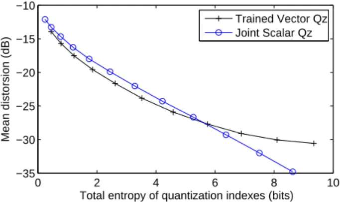
4.5. Performance on real audio data
We applied our quantizer to a corpus of EDS parameters ob-tained by analyzing real audio signals: 8 audio excerpts from various musical styles, sampled at 44.1kHz. We use the same analysis method as in [5]. In the preprocessing stage, the signal is segmented in variable-length time-segments aligned with onset positions in order to get physically consistent EDS parameters. But this is not directly related to the design of the quantization stage. We set a constant model order in each time-segment (K = 50), so that approximately 95% of the energy is captured. The analysis gives a corpus of 64000 sets of parameters. We also use a second database, similar to the first one, to train a VQ. As one can see on figure 4, the mea-sured entropy-distortion function for the joint-scalar quantizer is asymptotically similar to the one obtained with synthetic data. For the VQ, as explained in [7], the minimum achiev-able distortion is limited by the size of the training database, which penalizes the VQ in high resolution.
5. CONCLUSION
We considered the quantization of exponentially damped si-nusoids parameters. Given a constraint on the entropy of quantization indexes, i.e. the number of coding bits per sinu-soid, we proposed a new asymptotically optimal quantization
0 2 4 6 8 10 −35 −30 −25 −20 −15 −10
Total entropy of quantization indexes (bits)
Mean distorsion (dB)
Trained Vector Qz Joint Scalar Qz
Fig. 4. Entropy-Distortion function on real audio data.
scheme for amplitude, phase and damping. We showed that our method performs better than a more simple scheme, and almost as well as a trained vector quantizer, which is theoreti-cally the best solution, although practitheoreti-cally not suitable in the context of audio coding. We also showed that the additional damping parameter requires fewer coding bits compared to amplitude and phase. This suggests that the EDS model is an efficient alternative to constant amplitude sinusoidal models for parametric audio coding. However, this is still a work in progress: we will extend our study to include the quantiza-tion of frequency, and consider the repartiquantiza-tion of the coding bits between several sinusoids using a hearing model.
6. REFERENCES
[1] J. Nieuwenhuijse, R. Heusdens, and E.F. Deprettere, “Ro-bust exponential modeling of audio signals,” in Proc.
ICASSP’98, Seattle, WA, USA, May 1998.
[2] J. Jensen and R. Heusdens, “A comparison of sinusoidal model variants for speech and audio representation,” in
Proc. EUSIPCO’02, Toulouse, France, Sept. 2002.
[3] R. Vafin and W.B. Kleijn, “Entropy-constrained polar quantization and its application to audio coding,” IEEE
tr. Speech, Audio Process., vol. 13, no. 2, Mar. 2005.
[4] P. Korten, J. Jensen, and R. Heusdens, “High-resolution spherical quantization of sinusoidal parameters,” IEEE tr.
Audio, Speech, Lang. Process., vol. 15, no. 3, Mar. 2007.
[5] R. Badeau, R. Boyer, and B. David, “EDS paramet-ric modeling and tracking of audio signals,” in Proc.
DAFx’02, Hamburg, Germany, Sept. 2002.
[6] A. Gersho, “Asymptotically optimal block quantization,”
IEEE tr. Inf. Theory, vol. 25, no. 4, July 1979.
[7] P.A. Chou, T. Lookbaugh, and R.M. Gray, “Entropy-constrained vector quantization,” IEEE tr. Acoust., Speech, Signal Process., vol. 37, no. 1, Jan. 1989.