HAL Id: tel-01260398
https://tel.archives-ouvertes.fr/tel-01260398
Submitted on 22 Jan 2016
HAL is a multi-disciplinary open access archive for the deposit and dissemination of sci-entific research documents, whether they are pub-lished or not. The documents may come from teaching and research institutions in France or abroad, or from public or private research centers.
L’archive ouverte pluridisciplinaire HAL, est destinée au dépôt et à la diffusion de documents scientifiques de niveau recherche, publiés ou non, émanant des établissements d’enseignement et de recherche français ou étrangers, des laboratoires publics ou privés.
and control of smart grids
Davis Montenegro Martinez
To cite this version:
Davis Montenegro Martinez. Actor’s based diakoptics for the simulation, monitoring and con-trol of smart grids. Electric power. Universidad de los Andes (Bogotá), 2015. English. �NNT : 2015GREAT106�. �tel-01260398�
Pour obtenir le grade de
DOCTEUR DE L’UNIVERSITÉ GRENOBLE ALPES
préparée dans le cadre d’une cotutelle entre
l’Université Grenoble Alpes et L’Universidad de los
Andes
Spécialité : Génie Electrique
Arrêté ministériel : le 6 janvier 2005 - 7 août 2006 Présentée par
Davis / MONTENEGRO MARTINEZ
Thèse dirigée par Seddik/BACHAcodirigée par Gustavo Andrés/RAMOS LOPEZ préparée au sein des Laboratoire G2ELAB
dans les Écoles Doctorales l'École Doctorale Electronique, Electrotechnique, Automatique, Télécommunication et Traitement du Signal et le département du génie électrique et électronique de L’Universidad de los Andes
Diakoptics basés sur les acteurs pour la
simulation, la surveillance et la commande
des réseaux intelligents
Thèse soutenue publiquement le « 19 Novembre 2015 »,
devant le jury composé de :
M, Daniel, HISSEL
Professeur à l’Université de Franche Comté, Président
M, Damien, TROMEUR
Professeur à l’Université Claude Bernard Lyon 1, Examinateur
M, Gilney, DAMM
Maître de conférence à l’Université d’Evry-Val-d ‘Essonne, Examinateur
M, Mario Alberto, RIOS MESIAS
Professeur à L’Universidad de los Andes, Examinateur
M, Abdelkrim, BENCHAIB
Supergrid Institute (GE Grid Solutions) HDR\Professeur CNAM, Rapporteur
M, Ionel, VECHIU
Professeur \HDR à l’ESTIA, Rapporteur.
M, Seddik, BACHA
Professeur à l’Université Grenoble Alpes, G2Elab, Directeur de thèse
M, Gustavo Andres, RAMOS-LOPEZ
Professeur à L’Universidad de los Andes, Directeur de thèse
M, Roger, DUGAN
This Thesis is called Diakoptics based on actors for the simulation, control and monitoring of smart grid applications was developed in cotutel with the « Laboratoire de Génie Electrique de Grenoble » (G2ELab), France, and the Universidad de los Andes, Colombia.
First of all I want to say thanks to god the all mighty, because without him we are nothing and because he gave to my family and to me the strong and discipline to grow personally and intellectually during the development of this thesis.
I want also say thanks to my lovely wife: Luisa, you are a very important part on this process, your love, support and patience make possible all our goals as individuals and family. Also thanks for our beautiful son, who has arrived in the middle of this wonderful experience and gave us a new perspective of life, making us to realize as parents and human beings. This thanks are extensive to my parents Flor and Jorge and to my brothers Giovanny, Gino and Giorgio: guys, without your help, many of the things that I have reached in my life would not be possible.
I want to say thanks to my Colombian advisor, Mr. Gustavo Ramos, he has become a friend giving to me the opportunity to speak and propose ideas in a changing world. Gustavo, thanks for your support and for believe in this project since the beginning; together, we have passed a lot of adventures defending our ideas and proposing new paths to follow for the power industry and to leave our little mark in the world, thanks a lot.
Thanks a lot too to my French advisor, Mr. Seddik Bacha, who received me since my first moment in France as a father. Seddik, without your support, we maybe could not show the potential of our development and without your advice, I would not be able to understand that we are here not only for being the best, but for serving to the people around us with our talents and ideas.
I want to especially acknowledge to Mr. Roger Dugan and Mr. Mark McGranaghan and to the amazing team of the Electric Power Research Institute EPRI, all of you have seeded in me the need for going beyond of what it is established in the power industry, you also gave me the opportunity of being part of your team for a short period, but at the same time showed me the amazing and passionate world of research in this area. Roger, thanks a lot for believe in this initiative and for supporting us with this amazing tool called OpenDSS, which has served for supporting a good number of developments around the world and to give new ideas and innovative paths to engineers worldwide. Mark, you have been also an important and fundamental support for this project for believing is us and for giving us the opportunity to show what we are capable to do. Thanks a lot.
I want to thank to the Universidad Santo Tomas for supporting my formation during this period, particularly, I want to say thanks to the Engineer Adriana Cecilia Paez (Jefe), who has supported this project by giving me the time to finish it and for letting me to be part of the great group of the faculty of Electronics Engineering of this prestigious University. Also, I want to thank to the lab’s working team: Giovanni, William, Juancho, Javier, Jason and of course, Leonel Giraldo, to the university’s directives and the administrative personnel.
I want to say thanks to all the amazing people I have met during the development of this project. To my friends in the different parts of the world: Julian Fernandez, Jose L. Sanchez, Mariam Ahmed (and
Garcia, thanks for being such a nice persons with me and my family.
Finally, I want to thank to the Colombian government for supporting this thesis through the program “Becas para doctorados en Colombia” and the “Convocatoria 528, Colciencias”. Also, this acknowledgment is extensive to the working team of Colfuturo for their management talent during the development of this thesis.
GENERAL INTRODUCTION………...12
CHAPTER 1. INTRODUCTION TO POWER SYSTEMS SIMULATION IN REAL-TIME ... 13
CHAPTER 1 INTRODUCTION TO POWER SYSTEMS SIMULATION IN REAL-TIME ... 14
SIMULATION FIDELITY ... 15
Electromagnetic Transients (EMT) simulation ... 15
Load flow simulation (phasor simulation) ... 16
Hybrid simulation (phasor and EMT simulation) ... 17
SIMULATORS AND HARDWARE ... 17
Analog simulators ... 18
Digital simulators ... 19
Hybrid simulators ... 20
REAL-TIME SIMULATION AND ITS EVOLUTION ... 21
Addressing real life scenarios through Real-Time simulation ... 21
Power-Hardware-In-the-Loop simulators (PHIL) ... 23
Controller-Hardware-In-the-Loop simulators (CHIL) ... 23
CHALLENGES WHEN SIMULATING REAL-LIFE SCENARIOS ... 25
The evolution of computing systems ... 25
Multithread and vectorization ... 27
THE SCOPE OF THIS THESIS ... 28
CONCLUSIONS ... 29
CHAPTER2. SIMULATION OF DISTRIBUTION POWER SYSTEMS FOR SHAPING THE FUTURE SMART GRID ... 30
CHAPTER 2 ... 31
SIMULATION FOR THE DEVELOPMENT OF THE FUTURE SMART GRID ... 31
THE SOLUTION METHODS FOR LOAD FLOW ANALYSIS IN DS ... 32
Power flow analysis based on phase frame ... 32
Power flow analysis based on sequence frame ... 36
Dynamic Simulation ... 38
CHALLENGES FOR DS SIMULATION ... 41
The deterministic computing cycles ... 41
Complexity of the simulation ... 41
Topology changes ... 42
Hybrid power systems ... 42
CONCLUSION ... 42
CHAPTER3. DISTRIBUTION SYSTEM LOAD FLOW ANALYSIS USING DIAKOPTICS ... 43
The orthogonal networks ... 45
The interconnected equivalent network ... 50
THE MULTILEVEL APPROACH ... 52
Separating the Connections matrix ZCC ... 52
Distributing tasks ... 54
Simulation of Hybrid power systems... 55
THE COMPUTATIONAL MODEL OF DIAKOPTICS ... 57
Creating primitive networks (Islands) ... 58
Distributed computation ... 64
CONCLUSIONS ... 65
CHAPTER 4. THE ACTOR MODEL FOR HANDLING PARALLEL AND CONCURRENT COMPUTING ... 66
CHAPTER 4 ... 67
INTRODUCTION TO THE ACTOR MODEL ... 67
Homogeneous and Heterogeneous computing systems ... 68
Actors and Agents ... 70
BUILDING AN ACTOR’S SYSTEM ... 71
The actor structure ... 71
The actor messages ... 73
The management of the hardware resources ... 74
The standard PC architecture ... 74
The Real-Time Architecture ... 75
ACTOR’S ENVIRONMENT PROPOSED FOR IMPLEMENTING A-DIAKOPTICS ... 76
The parent actor architecture ... 78
The child actor architecture ... 80
The messages architecture ... 82
CONCLUSIONS ... 82
CHAPTER 5. APPLICATIONS OF A-DIAKOPTICS ... 84
CHAPTER 5 ... 85
APPLICATIONS OF A-DIAKOPTICS ... 85
THE SIMULATION OF DISTRIBUTION POWER SYSTEMS... 85
Distribution System Simulation using Standard PC architectures ... 86
The harmonics simulation mode ... 88
The sequential-time TSA ... 90
Performance of the PC application ... 91
Distribution System Simulation using Real-Time architectures ... 100
OTHER FUTURE APPLICATIONS ... 105
DS state estimation ... 105
Advanced Distribution Automation ... 108
GENERAL CONCLUSIONS ... 111
Figure 1-1. Cost trend when detecting bugs in different stages of a product development. ... 14
Figure 1-2. Simulated phenomena using EMT simulation (based on the graph provided in (Watson et al., 2003)) ... 15
Figure 1-3. Simulated phenomena using phasor simulation (based on the graph provided in (Watson et al., 2003)) ... 16
Figure 1-4. 39-bus New England AC system with two HVDC links (Xi et al., 2009) ... 17
Figure 1-5. Test system implemented using an analog simulator (Imai et al., 2002). ... 18
Figure 1-6. Hybrid simulator example ... 20
Figure 1-7. Uses of Real-time simulators for addressing real world applications. ... 22
Figure 1-8. HIL Power system simulation categories. ... 24
Figure 1-9. Classical sequential computing systems ... 25
Figure 1-10. Multicore computing systems ... 26
Figure 1-11. Application fields of parallel computing (Jainschigg, 2012) ... 27
Figure 2-1. Solution methods used for power flow analysis in DS ... 38
Figure 2-2. Dynamic behavior of voltage (p.u.) after the disconnection and reconnection of a 1MW generator from EPRI’s circuit 7- 2452 nodes. Step time 4.5 ms. Graph generated with DSSim-PC (Montenegro, 2013). ... 41
Figure 3-1. Link branch of an electrical system ... 45
Figure 3-2. System under study ... 45
Figure 3-3. YBUS matrix for modeling the proposed system ... 46
Figure 3-4. YBUS matrix after switch SW_1 trips ... 46
Figure 3-5. YBUS reorganized after switch SW_1 tripping ... 47
Figure 3-6. Transposed contour matrix in the case presented in Figure 3-5 ... 48
Figure 3-7. Example of reference frame moving using a transformation matrix. In this case, matrix A is the transformation matrix for taking matrix B from the domain YY to the domain XX. .... 49
Figure 3-8. Equivalent ZTT matrix obtained from the tree admittance matrix YTT ... 50
Figure 3-9. The proposed procedure for solving the interconnected equivalent (physical interpretation) ... 50
Figure 3-10. Two power systems represented using their interconnected equivalents in Diakoptics. F1 and F2 means that both systems are operating at different base frequencies. .... 56
Figure 3-11. Two power systems working at different base frequencies combined into a single Diakoptics structure ... 56
Figure 3-12. A control model for interconnecting two power systems working in different base frequency. ... 57
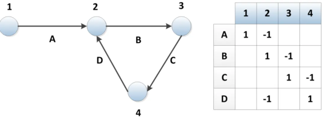
Figure 3-13. The network represented as a graph and its incidence matrix ... 59
Figure 3-14. The set of nodes strongly connected and their adjacent matrix. ... 59
Figure 3-15. Proposed iterative algorithm for detecting and reorganize islands within sparse matrixes ... 60
Figure 3-16. The proposed system to evaluate the performance of the proposed algorithm... 61
Figure 3-17. IM obtained for the study case 1 ... 61
Figure 3-18. YBUS matrix obtained for the case of study 1 ... 61
Figure 3-19. IM obtained for the study case 2 ... 62
Figure 3-22. YBUS matrix obtained for the case of study 3 ... 63
Figure 3-23. IM obtained for the study case 4 ... 63
Figure 3-24. YBUS matrix obtained for the case of study 4 ... 63
Figure 3-25. The hierarchical computation model proposed for implementing Diakoptics ... 64
Figure 3-26. The interconnected network in Figure 3-2 (a) and its electrical equivalent using Diakoptics (b) ... 65
Figure 4-1. Project tree for creating an actor using NI LabVIEW ... 71
Figure 4-2. State Machine structure ... 72
Figure 4-3. Functional actor core created using NI LabVIEW (running under regular Windows OS) ... 73
Figure 4-4. Functional actor implemented for RT execution (running under Windows embedded OS) ... 75
Figure 4-5. New parameters required for actor’s RT execution (running under Windows embedded OS) ... 75
Figure 4-6. Actor framework proposed for implementing the A-Diakoptics methodology ... 76
Figure 4-7. Hierarchical actor’s model proposed for implementing A-Diakoptics ... 77
Figure 4-8. Expected interactions between actors ... 77
Figure 4-9. State machine proposed for the parent actor ... 80
Figure 4-10. State machine proposed for the child actor ... 81
Figure 5-1. Actor framework proposed for DSSim-PC ... 86
Figure 5-2. Load model in harmonics mode (Dugan et al., 2014) ... 88
Figure 5-3. Content of the child actors when working in harmonics mode ... 89
Figure 5-4.Harmonics meter graphical panel ... 90
Figure 5-5. Exchange methodology to include new models in the simulation ... 90
Figure 5-6. Medium-scale (a) and large-scale (b) DS modeled in DSSim-PC using the translator from .DSS to .DSP. Network (a) has one layer and network (b) has two layers. ... 92
Figure 5-7. Layers model for representing small-scale, medium-scale and large-scale power systems ... 93
Figure 5-8. Simulation time for executing 1 iteration on DSSim-PC and OpenDSS ... 94
Figure 5-9. Testing scenario using DSSim-PC ... 95
Figure 5-10. Testing scenario using OpenDSS ... 95
Figure 5-11. Results obtained in test scenario 2 ... 95
Figure 5-12. Results when simulating 10000 iterations with OpenDSS and DSSim-PC (Graphical) ... 97
Figure 5-13. Computing time improvements (percentage) reached when using A-Diakoptics within PC architectures ... 98
Figure 5-14. Measurements taken at different points of EPRI’s circuit 7 in dynamic simulation, graphic generated with DSSim-PC (Torsional mode oscillations)- 1.5 sec ... 98
Figure 5-15. Torsional mode oscillations in Voltages (p.u.) provided by DSSim-PC and OpenDSS at node x_1001805 - phase A, 2 sec ... 99
Figure 5-16. Multirate waveform generated by mixing the data and carrier signals ... 99
Figure 5-17. Data waveform and combined waveform (data + carrier) for reproducing the voltage signal according to the data generated. ... 100
Figure 5-18. Actor framework proposed for DSSim-RT ... 101
Figure 5-19. Heterogeneous computing environment proposed for implementing DSSim-RT 102 Figure 5-20. Performance comparison between PC and RT simulators using A-Diakoptics ... 102
oscillations. Phase A ... 103
Figure 5-22. Simulation time (1 iteration) of the IEEE 8500 node test system simulated using several cores ... 104
Figure 5-23. Comparison between the measured times and estimated times using equation 5.2 ... 104
Figure 5-24. Projection for estimating the behavior of the system processing time when the number of cores on the simulation increases ... 105
Figure 5-25. Latencies by using a communication network to communicate with IEDs ... 106
Figure 5-26. Classical methodology for gathering data from distributed meters (Agents) ... 107
TABLE 1-1 ... 19 TABLE 2-1 ... 33 TABLE 2-2 ... 33 TABLE 2-3 ... 34 TABLE 2-4 ... 35 TABLE 2-5 ... 35 TABLE 2-6 ... 36 TABLE 2-7 ... 37 TABLE 2-8 ... 38 TABLE 2-9 ... 39 TABLE 3-1 ... 52 TABLE 3-2 ... 54 TABLE 4-1 ... 69 TABLE 4-2 ... 82 TABLE 5-1 ... 91 TABLE 5-2 ... 91 TABLE 5-3 ... 93 TABLE 5-4 ... 96 TABLE 5-5 ... 97 TABLE 5-6 ... 101
12 The simulation of power systems is an important tool for designing, developing and assessment of new grid architectures and controls within the smart grid concept for the last decades. This tool has evolved for answering the questions proposed by academic researchers and engineers in industry applications; providing different alternatives for covering several realistic scenarios.
Nowadays, due to the recent advances in computing hardware, Digital Real-Time Simulation (DRTS) is used to design power systems, to support decisions made in automated Energy Management Systems (EMS) and to reduce the Time to Market of products, among other applications.
Power system simulations can be classified in the following categories: (1) Analog simulation (2) off line simulation (3) Fully digital simulation (4) Fast simulation (5) Controller Hardware-In-the-Loop (CHIL) simulation and (6) Power Hardware-In-the-Loop (PHIL) simulation.
The latest 3 are focused on Real-Time Hardware-In-the-Loop (RT-HIL) simulation. These categories cover issues related to Electromagnetic Transients (EMT), phasor simulation or mixed (phasor and EMT). As mentioned above, these advances are possible due to the evolution of computing architectures (hardware and software); however, for the particular case of power flow analysis of Distribution Systems (DS) there are still challenges to be solved.
The current computing architectures are composed by several cores, leaving behind the paradigm of the sequential programing and leading the digital system developers to consider concepts such as parallelism, concurrency and asynchronous events. On the other hand, the methods for solving the dynamic power flow of distribution systems consider the system as a single block; thus they only use a single core for power flow analysis, regardless of the existence of multiple cores available for improving the simulation performance.
Divided into phase and sequence frame methods, these methods have in common features such as considering a single sparse matrix for describing the DS and that they can solve a single frequency simultaneously.
These features make of the mentioned methods non-suitable for multithread processing. As a consequence, current computer architectures are sub-used, affecting simulator's performance when handling large scale DS, changing DS topology and including advanced models, among others real life activities.
To address these challenges this thesis proposes an approach called A-Diakoptics, which combines the power of Diakoptics and the Actor model; the aim is to make any conventional power flow analysis method suitable for multithread processing. As a result, the nature and complexity of the power system can be modeled without affecting the computing time, even if several parts of the power system operate at different base frequency as in the case of DC microgrids. Therefore, the dynamic load flow analysis of DS can be performed for covering different simulation needs such as off-line simulation, fast simulation, CHIL and PHIL. This method is an advanced strategy for simulating large-scale distribution systems in unbalanced conditions; covering the basic needs for the implementation of smart grid applications.
13
Chapter 1. Introduction to Power Systems
Simulation in Real-time
CHAPTER 1. INTRODUCTION TO POWER SYSTEMS SIMULATION IN REAL-TIME ... 13
CHAPTER 1 INTRODUCTION TO POWER SYSTEMS SIMULATION IN REAL-TIME ... 14
SIMULATION FIDELITY ... 15
Electromagnetic Transients (EMT) simulation ... 15
Load flow simulation (phasor simulation) ... 16
Hybrid simulation (phasor and EMT simulation) ... 17
SIMULATORS AND HARDWARE ... 17
Analog simulators ... 18
Digital simulators ... 19
Hybrid simulators ... 20
REAL-TIME SIMULATION AND ITS EVOLUTION ... 21
Addressing real life scenarios through Real-Time simulation ... 21
Power-Hardware-In-the-Loop simulators (PHIL) ... 23
Controller-Hardware-In-the-Loop simulators (CHIL) ... 23
CHALLENGES WHEN SIMULATING REAL-LIFE SCENARIOS... 25
The evolution of computing systems ... 25
Multithread and vectorization ... 27
THE SCOPE OF THIS THESIS ... 28
14
Chapter 1 Introduction to Power Systems
Simulation in Real-time
For several decades the simulation of power systems has been the main tool for designing, developing and assessing new technologies within the smart grid concept (Caixue, Kaldewey, Povzner, & Brandt, 2006; Ren et al., 2011). This tool is the source for answering the questions proposed by nowadays society by academic researchers and engineers in industry applications (Chang, Liu, Dinavahi, & Ke, 2008; Cheng & Shirmohammadi, 1995), which has generated a constant demand for making evolve these systems in order to cover a wide spectrum of realistic scenarios.
Nowadays, due to the recent advances in computing hardware, Digital Real-Time Simulation (DRTS) is used to design power systems, to support decisions made in automated Energy Management Systems (EMS) and to reduce the Time to Market release of products, among other applications (Dufour & Belanger, 2006; Dufour, Hoang, Soumagne, & El Hakimi, 1996; Fernandes et al., 2012). Moreover, each type of simulation has its own requirements in terms of performance, interface and hardware.
As an expected result of using simulations, the negative impact that new technologies could generate when they are integrated into a working system should be minimized. In fact, several studies reveal that depending on the development stage of a product, detecting an error could represent important economic issues (Soni, 2015). As shown in Figure 1-1, when developing a new technology the detection of bugs in the right moment could symbolize an important success; at the opposite side, if these bugs are not detected this new technology could represent a big economic disaster when trying to enter into the market competition (Harter, Krishnan, & Slaughter, 2000; Shull, Rus, & Basili, 2000). For these reasons, Real-Time simulation has gained an important part of the simulation market in the recent years. Due to their flexibility and because they provide more information about the performance of a project or product in a test that can be destructive in real life, Real Time simulation is now the preferred tool for manufacturers and for the industries such as aerospace & defense, automotive, electrical and academic research among others (de Jong, de Gelder, Bussink, Verhoeven, & Mulder, 2013; Landry & Pritchett, 2002).
Figure 1-1. Cost trend when detecting bugs in different stages of a product development.
Construction Detailed design ArchitectureRequirement Stag e in which the bu g is g enerated Trend of the econ omic cos t
15 However, the scope of the simulation could vary depending on the type industry and the application field to simulate; these needs define the features of the simulation such as step time, computing power required, dynamic and generated signals. Based on these features, the simulation of power systems addresses several phenomena and their use could be oriented to different functional applications such as design and modeling, rapid prototyping, testing, teaching and training.
Simulation fidelity
In general, the aim of the Power system’s simulation is the prediction of the technical limits that can produce stress to the components interconnected within the power system, such as power quality disturbances, frequency problems, voltage stability issues, among others. These phenomena can be predicted using different techniques depending on the scope of the simulation.
Electromagnetic Transients (EMT) simulation
Electromagnetic Transient simulation (EMT) refers to highly accurate simulations where the aim is to reproduce the behavior of the power signal when disturbed by high speed electromagnetic events. This type of simulation is time based and its timescale could vary from microseconds to nanoseconds, which makes of it highly demanding in terms of computational performance (Watson, Arrillaga, & Engineers, 2003).
EMT simulation involves primarily the interactions between the magnetic fields of inductances and the electric fields of capacitors connected to the power system, which can be generated by several causes as shown in Figure 1-2. As can be seen in this Figure, the time scale can drastically change depending on the type of phenomena to simulate; this feature will increase the complexity of the simulation in terms of computational burden and required hardware resources. For this reason, the EMT simulation in Real-Time normally involves small and medium-scale power systems interfaced using control devices such as VSCs in hybrid power systems, distributed generation (Missaoui, Warkozek, Bacha, & Ploix, 2012), HVDC systems (transmission systems), protections, among others (Rogersten, Vanfretti, Wei, Lidong, & Mitra, 2014; Yi, Gole, Wenchuan, Boming, & Hongbin, 2013; Yin, Haixiang, Ying, & Chen-Ching, 2014). The solution of EMT simulation is based on first order differential equations using Kirchhoff’s laws for describing the behavior of RLC circuits when excited by a specific stimulus (Mekhtoub, Ibtiouen, Touhami, & Bacha, 2007).
16
Load flow simulation (phasor simulation)
On the other hand, load flow simulation is focused on study the electromechanical transients. These transients are given due to the interactions between the energy stored in rotating machines, and the electrical energy stored in the grid. This type of simulation has a bigger time scale than in the case of EMT, but its field of application and he phenomena modeled demands this treatment.
This simulation is also called phasor simulation because is based on phasors to determinate the state of the power system instantaneously; however, this type of simulation can be translated to the time domain using sequential time simulation, which allows to incorporate the dynamic behavior of the power conversion devices for evolving into a type of simulation called transient stability programs or Transient Stability Analysis programs (TSA) (Sankarakrishnan & Billinton, 1995). This feature also has encouraged the development of simulation models for harmonic studies (Dugan, Arrit, Henry, McDermott, & Sunderm, 2014); complementing the load flow simulation for recreating short and long term variations of power quality (McDermott & Dugan, 2003; Montenegro, Hernandez, & Ramos, 2015; Montenegro & Ramos, 2012; Ramos & Montenegro, 2012).
The time scale of this type of simulation goes from milliseconds to weeks, months or years, but instead of EMT simulation, the scale of the power systems simulated can be large. The load flow simulation has been used mainly for analyzing the behavior of Distribution Systems due to its unbalanced nature; this feature increases the complexity for solving the system at computational level because of the size of the equations, which are modeled as a square matrix using nodes while in transmission systems, the model is balanced and analyzed using buses (Abdel-Akher, Nor, & Rashid, 2005; Stott, 1974).
The phenomena studied with this kind of simulation are shown in Figure 1-3. The control devices for this kind of simulation can be HVDCs, VSCs, generation controllers, protections, prime mover controllers, Load Frequency Controllers (LFC) and in general, the result of operations performed from the EMS.
17
Hybrid simulation (phasor and EMT simulation)
Transient Stability Analysis do not require the same accuracy in the time domain than in the case of EMT. In TSA, the solution is based on a single frequency (one frequency per solution) using phasors; however, in the last years, several advances for integrating TSA and EMT simulations have been developed; the aim is to reduce the computational burden by focusing the EMT approach on a certain part of the system such as HVDCs, FACT, and leave the rest of the power system to the TSA approach.
In hybrid simulation is necessary to tolerate the reduced precision for transients that could happen in the EMT simulation, which is the result of the electrical interaction between the EMT and the TSA components and due to EMT is a multi – rate type of simulation. This feature is acceptable for pure AC systems, but when the system is a hybrid AC/DC system large errors can compromise the fidelity of the simulation (Xi, Gole, & Ming, 2009; Yizhong, Wenchuan, Boming, & Qi, 2013).
For solving this challenge, several authors have proposed the integration of a Frequency Dependent Network Equivalent (FDNE) for interfacing the TSA and EMT components; this approach looks for preserving the accuracy of the EMT part by adding equivalent representations (Xi et al., 2009). An example of a system suitable for hybrid simulation is shown in Figure 1-4.
Figure 1-4. 39-bus New England AC system with two HVDC links (Xi et al., 2009)
The simulation fidelity is also affected by the hardware used for recreating the simulated scenario, which has evolved for covering the needs of the industry and academia looking for modularity, flexibility and scalability.
Simulators and hardware
According to the hardware used for recreating realistic scenarios, simulators can be separated into analog and digital simulators. The first case consists of building reduced models that approximates the real system behavior; on the other hand, digital simulators are computing programs used for solving differential equations and recreate the behavior of the power system (Roitman, Watanabe, & Lyra, 1989). Both are described as follows.
26 28 29 27 25 2 3 18 17 16 19 23 22 21 24 15 14 13 10 4 5 6 7 8 G38 G33,G34 G36 G35 External System Bus #3 Bus #8 G32 G31 Gen #37 G30 DC LINK 1 DC LINK 2 Internal System
18
Analog simulators
The concept of analog simulators is composed by two different approaches: The construction of reduced models using electrical elements for reproducing the behavior of a real system, and the inclusion of active electronic circuits to overcome speed limits in digital simulators (analog computations) (Nagel, Fabre, Cherkaoui, & Kayal, 2010). Classically, this kind of simulator is the base for practicing in laboratories and teaching due to its similarity to the studied phenomena (Imai, Iizuka, Makino, & Horikoshi, 2002). However, when the study case becomes medium/large-scale with hundreds of elements and complex cases, the costs associated with this kind of simulators can increase drastically and the complexity of the implementation as well.
The advantage when working with analog simulators is that there are no delays when performing the tests. On the other hand, the flexibility of the recreated scenarios using this technique is limited because of the components used are too specific, leading to prefer other simulation techniques (Gombert, 2005):
The size of the systems that can be represented is limited due to the complexity of the scenarios to be recreated.
The flexibility, modularity and scalability of these kind of simulators is also limited due to the amount and type of components required for the simulation. In fact, sometimes the stress experienced by these components require to have a replacement for each component depending on the number of iterations required for gathering data (Braham, Schneider, & Metz, 1997).
The values and type of the components required for recreating a certain scenario are specific, which makes of the simulator uniquely and not suitable for creating other experiments.
An example of a test system implemented using an analog simulator is shown in Figure 1-5(Imai et al., 2002).
19
Digital simulators
Digital simulators are computer based and consist in algorithms for solving linear and nonlinear equations in order to reproduce the behavior of the physical system. These simulators can work off-line, on-line and Real-time for recreating different scenarios (Ren et al., 2011; Wang, Guo, Xiao, & Zhao, 2010). The precision and fidelity of these simulators depends on the computing hardware architectures and interfaces. Some of these can be used for collecting data without any interaction with the real world, while some others can be used for interacting with devices under test (DUT) or hardware under test (HUT); closing the simulation loop using Digital to Analog Converters (DAC) or communication interfaces (Dufour & Belanger, 2006; Dufour, Belanger, & Lapointe, 2008).
Driven using software interfaces, the main feature of this kind of simulator is that the simulation becomes flexible, modular and scalable; nevertheless, depending on the hardware characteristics the spectrum of the simulated signals can vary (Ocnasu, 2008; Ren et al., 2011).
Nowadays, this type of simulation is the preferred by the power industry and academia; addressing a wide spectrum of applications and issues related to the development of new control and monitoring devices for building the modern power grids (Zhong et al., 2013). In TABLE 1-1, a list of the most representative manufacturers of digital simulators for TSA/EMT is presented.
TABLE 1-1
MOST RECOGNIZED SIMULATION TOOLS AVAILABLE NOWADAYS
Company Product name Type of simulation License
DigSilent Power Factory Off Line/On-line Paid
Manitoba Hydro International Ltd. PSCAD/EMTDC Off Line Paid
International Power Electric Technology
Co. CYMDIST Off Line Paid
WH Power consultants RDAP Off Line Paid
Matworks SimPower Systems MATLAB Off Line Paid
Battelle Memorial Institute GridLab-D Off Line Freeware
EPRI OpenDSS Off Line Open
Source
Stanford University GridSpice/
GridLab-D Off Line
Open Source
Operation Technology, Inc. etap Off Line/Real-Time Paid
Opal-RT ePHASORSim Real-time Paid
RTDS RSCAD-GTNET-PMU Real-time Paid
20
Hybrid simulators
For addressing the limits identified in analog and digital simulators, the hybrid simulator combines their strengths for evolving into an advanced simulation platform. This simulator combine the fidelity of the analog simulators with the models recreated in the discrete time domain using digital systems (Gick, Gallenkamp, & Wess, 1996). Hybrid simulators are used for exchanging signals between the discrete and continuous worlds, and explore the different states that a new device require for addressing the different functional states of the power system (Zhu, Dong, Hu, & Xie, 2013).
For interfacing the digital and analog simulators it is required the inclusion of power amplifiers and DACs; this way, highly complex equipment can be simulated using analog simulators while the rest of the power system is recreated digitally. The literature reports applications such as testing of HVDC interfaces, the interconnection of distributed generators to analog HVDC systems, the testing of dynamic loads simulated digitally and connected to analog power systems, among others. A general example of a hybrid simulator is shown in Figure 1-6.
Depending on the application, the voltages and currents gong from the Digital simulator to the Analog Simulator and vice versa can vary. For example, consider an experiment where a set of controllers are simulated using the digital simulator and the power system with the Analog one. In this case, the voltage and current signals goes from the analog simulator to the digital and if necessary, the Digital part will feedback some processed signals.
Another example could be when a large-scale DS is simulated in the Digital simulator and a small part of the big system is simulated using the Analog simulator, which is used for recreating power quality issues and interconnect real controllers; then, the results of the control actions and the disturbances generated in the Analog simulator are entered into the Digital simulator for feeding back the entire power system in the next iteration. These kind of simulators are Real-time driven, which is the subject of the next section.
21
Real-time simulation and its evolution
Real-time simulation is the preferred tool for designing, testing and assessing new technologies and products in the last decades. This kind of simulation allows to recreate the real world using computing hardware, which can be interfaced with real equipment/system for evaluating its performance before being installed in real the real world (Laplante & Ovaska, 2011).
A Real-time (RT) computer system is a computer system where the functional state of this system is not only linked to the compute cycles, but also on the physical time required for performing these computations. The functional states refer to the input/output cycles of the system. So, RT systems are time dependent digital systems that evolve in time according to a fixed period, ruled by a global clock (Kopetz, 2011).
These computers are always part of a larger system called RT systems or cyber-physical systems due to its dependence of physical-time. The general structure of an RT computer is distributed in computer nodes interconnected by a RT communication network (Kopetz, 2011). The time definitions that rule the RT system are described as follows:
A cut in the timeline is called an instant.
Any ideal occurrence that happens at an instant is called an event. The information that describes the event is called the event information.
The present (now) is the reference point used for separating the past from the future.
An interval on the timeline is called duration and is defined by two events (start and terminating)
Because the system is referenced to a digital clock, the timeline is partitioned into a sequence symmetrically spaced, each space is called granules of the clock, which are delimited by special periodic events called ticks of the clock.
These definitions will be used for describing the operation of the RT simulators and their features for addressing different applications.
Addressing real life scenarios through Real-Time simulation
The advantage of RT simulators is the fact that computations are governed by deterministic computing times, which allows to ensure the response of the system to events produced in the continuous time domain with an accurate approach from the discrete time domain (Proakis & Manolakis, 1995; Tan, 2007). This way, real world scenarios can be recreated for testing, design and assessment of new technologies in the laboratory by offering high scalability, modularity and flexibility.
This tool has been used for recreating a large number of real world situations, the following are documented cases when RT simulators have been used in the power systems industry:
Design and testing of electric vehicles and storage devices (Dufour & Belanger, 2006; Yuhe, Wenjia, Kobayashi, & Shirai, 2012).
Design and validation of adaptive protection systems (Abdulhadi, Coffele, Dysko, Booth, & Burt, 2011; Crăciun et al., 2014).
Harmonics studies (Chang et al., 2008).
Switching transient studies (Bacha Seddik, 2014; Deokar, Waghmare, & Takale, 2009). Design and testing of transmission lines (Dufour et al., 1996).
22 Dynamic simulations for transmission and distribution power systems (Jalili-Marandi, Ayres,
Ghahremani, Belanger, & Lapointe, 2013).
The testing of Power Quality monitoring systems (Montenegro et al., 2015; Radil, Ramos, Janeiro, & Serra, 2008).
Development of interfaces for hybrid power systems (AC-DC links) (Zhu et al., 2013). Validation of building management strategies (Missaoui et al., 2012).
Studies for evaluating the dynamic behavior of interconnected distributed generators (Palensky & Dietrich, 2011; Yizhong et al., 2013).
Validation of information models for handling information through a network with distributed control devices (Zavoda, 2008; Zhong et al., 2013).
Studies about peak load shaving using Distributed Energy Resources (Van-Linh, Tuan, Bacha, & Be, 2014).
To evaluate non-intrusive load monitoring strategies (K. Basu, Debusschere, Bacha, Maulik, & Bondyopadhyay, 2015; Kaustav Basu, Debusschere, Douzal-Chouakria, & Bacha, 2015). To evaluate the performance of Real-Time estimation algorithms on DFIG and other rotational
machines and stability analysis (A. Djoudi, H. Chekireb, E. Berkouk, & S. Bacha, 2014; A. Djoudi, H. Chekireb, E. M. Berkouk, & S. Bacha, 2014).
Power optimization studies on Distributed Energy Resources (Taraft, Rekioua, Aouzellag, & Bacha, 2015).
Demand side optimization studies on Distributed Energy Resources (Thiaux, Dang, Multon, Ben Ahmed, & Tran, 2015).
And many others…
As can be seen in the previous list, the nature of the scenarios developed using RT simulation can vary significantly even if all of them are part of the same field of application, which has led to classify the RT simulators in two categories for interfacing them with real world devices in a closed simulation loop called Hardware-In-the-Loop (HIL). This concept is illustrated in Figure 1-7.
23
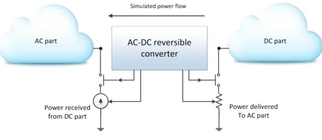
Power-Hardware-In-the-Loop simulators (PHIL)
Power-Hardware-In-the-Loop (PHIL) is a Hardware/Software HIL technique where the exchange of information between the RT simulator and the real world is made through analog power signals. The main parts of this hybrid simulator are the power amplifier and the signal conditioning interfaces (Lundstrom, Shirazi, Coddington, & Kroposki, 2013). Because the aim of this technique is to simulate power conditions for driving the external systems to a functional state, the interfaces with the real world generates separate voltage and current signals; thus making easier to test and to evaluate the system response when a certain event occurs (Dargahi, Ghosh, Ledwich, & Zare, 2012; Lundstrom, Mather, Shirazi, & Coddington, 2013). Here, the element under study is the entire power system and its behavior in time.
However, for using this technique and selecting the elements involved in the process, there are several considerations that must be deliberated before implementing an experiment (Ocnasu, 2008):
The nominal values of the waveforms, which must be considered in selecting properly the magnitudes of the interface and the operation ranges. If these values are not considered undesired effects could be part of the test such as saturation, protections tripping, malfunctioning of loads and connected equipment and the destruction of data acquisition devices.
The compatibility between the voltage levels between the analog and digital parts must be guaranteed. The gaining of the data acquisition devices and the gain levels of the power amplifiers must be coherent for avoiding accidents.
The operation range of all the elements must be well defined. With this consideration it is expected to avoid damage on the elements used.
The bandwidth of each element must be in the range established for the experiment.
It is important to know the response time of the elements included in the simulation; this way, the step time of the simulation will be selected for avoiding unpredictable behaviors and undesired noise or signal shifting.
Due to the nature of the simulations where the power flow can change product of a switch tripping to include reversible power conversion devices, distributed generators, among others. For these reasons it is necessary that the power amplifier could work in the four quadrants with a sufficient bandwidth.
Controller-Hardware-In-the-Loop simulators (CHIL)
On the other hand, Controller-Hardware-In-the-Loop (CHIL) is a technique where the interaction with external equipment is made through communication interfaces (Steurer, Bogdan, Ren, Sloderbeck, & Woodruff, 2007). This is because nowadays power networks transport not only power, but also data, which is transmitted using field buses and protocols for driving monitoring and control operations such as feeder reconfiguration, fault detection and isolation, Volt/VAr control, among others (Zavoda, 2008, 2010).
These kind of simulation is widely used for Phasor Measurement Unit (PMU) placement, for assessing power system management activities related to Electric Vehicles (EV), Electronic power converters (Lucia et al., 2011), Storage Devices and distributed generation penetration (Yuhang, Hui, & Foo, 2009). Advanced Distribution Automation (ADA) is as well, another topic studied when using these kind of simulators (Zavoda, 2010).
24 At a difference of PHIL, the controllers in CHIL are external equipment, replacing the simulated controllers present in PHIL (Yousefpoor, Parkhideh, Azidehak, & Bhattacharya, 2014), which means that the element under study is the controller. The communication protocols most used in these applications are:
Protocols
o CAN-Based on CAN bus o ModBus (RTU,ASCII, TCP-IP) o IEC61850 o CS104 o XMPP Field Buses o Optical Fiber o Ethernet o GPRS/GSM
o ZigBee oriented solutions (for closer locations) o RS485 (near to the end points)
o CAN/ASi
Figure 1-8. HIL Power system simulation categories.
Figure 1-8 presents an application example of the different HIL techniques used for simulating power systems. These developments are possible due to the evolution of the computing architectures, which have evolved through time passing from sequential to parallel systems; involving concepts such as concurrency and asynchronism to the development of RT simulators. These topics are presented in the next section.
25
Challenges when simulating real-life scenarios
As mentioned above, digital RT simulators are highly dependent of the computing available technology. The features of each simulator are directly associated to the hardware and software architectures used for its development.
For covering the needs in terms of performance and determinism of the simulation platforms described at this point, computer architectures have evolved from large to smaller computing hardware, which is more efficient and faster; however, these computers also require advanced programming structures at software level for exploiting all its power, requesting from RT systems developers to leave behind the paradigm of sequential programing (Abbas & Ahmad, 2002).
The evolution of computing systems
At the beginning of computing science, the computing systems have been designed for working sequentially. This trend prevailed until the beginning of the 21th century, which has led the software development tools to follow a vertical structure for using central-processing-units (CPU) working at fast rates. The features of this type of architecture are (Barney, 2014):
A problem is decomposed into a sequential set of instructions.
The instructions are executed sequentially (only one instruction was executed at the same time)
There is only one processor for handling all the instructions
This computing methodology was used for decades, but conforming the industry and academic researchers needs higher fidelity and lower computing times, hardware manufacturers were forced to develop faster processors for keeping the sequential processing methodology (Diaz, Munoz-Caro, & Nino, 2012b).
However, this hardware acceleration has reached its limits when hardware manufacturers realize that the heat and stress on the components started to become critical. So, new developments for reaching lower computation times and recreate accurately the real world were redirected to distribute tasks, is then when the parallel processing is needed. These concepts are illustrated in Figure 1-9.
26 The first parallel systems were built using computer networks interconnected using communication systems. These systems are known as heterogeneous computing systems due to the diversity of technical specification of the distributed computers (Hewitt, 1976; Hewitt & Barker, 1977). Even if all the computers have the same technical specifications and were manufactured by the same company in the same production batch, there are small differences that make each one unique, requiring to establish controls for guaranteeing synchronism, stability and inconsistency robustness in the same computation granule (Hewitt, 2012).
Then, thanks to the high integration and miniaturization techniques, groups of processors are integrated within the same structure, entering in the multi and many-core computing era (Diaz, Munoz-Caro, & Nino, 2012a). This processors are known as homogeneous computing systems and are very common nowadays, they can be found in every computer no matter the application field. The technical features of this technology are:
A problem is separated into discrete parts for being handled concurrently. Each part is later broken into a sequential set of instructions.
The instructions are executed sequentially on each core (more than one instruction was executed at the same time)
Global control/coordination mechanism must be employed for handling the operations performed by each core and coordinate the exchange of data between them.
For making this processing possible the problem to solve should be able to be broken into discrete pieces, considering multiple program instructions at any moment in time and as a consequence, the problem will be solved in less time than with a classical sequential computing system. Nevertheless, many of the computing software keeps being developed using sequential programming structures, which sub-utilize the power of parallel computing due to the program will use a single core for its execution.
Parallel processing is the alternative for recreating the real world, which is massively parallel. In the natural world many events are happening at the same time preserving a temporal sequence, and compared with sequential programming, parallel programming is more adequate for modeling, simulating and explaining real world phenomena (Barney, 2014; Schlesinger, 2010). These concepts are illustrated in Figure 1-10.
27 For handling parallel computing structures, the processor uses threads, which are also known as virtual processors within the physical processor. A thread can be described as a recipe delivered by parts to different chefs in a kitchen; there is no order for developing each part of the recipe and each chef works independently. Then when each part is ready each chef provides his part for building the total recipe (Inoue & Nakatani, 2010). However, for avoiding a chaotic kitchen, a leader chef is needed for coordinating the kitchen operation. In fact, multicore processing is called multithread, because is the thread the base entity for distributing processes within a core (Jainschigg, 2012).
Additionally, by the introduction of Fast Programmable Gate Arrays (FPGAs), the hardware can be described using hardware interfaces such as Very High speed Hardware Description Language (VHDL), opening the possibility for RT developers to customize their own hardware for developing specialized functions in high deterministic computing times (Brant & Lemieux, 2012; Dufour et al., 2008).
Figure 1-11. Application fields of parallel computing (Jainschigg, 2012)
Parallel programming/computing is widely used in several industries and application fields. Figure 1-11 provides an example of the application sectors where parallel computing is used nowadays (Jainschigg, 2012).
Multithread and vectorization
For handling parallel computing resources there are two methodologies proposed in the literature: Multithreaded programming
28 Multithreaded programming has existed for decades, in fact, the single-core processors on the early days used threads successfully for handling multiple tasks. For handling threads, the processor halts one thread for allowing the execution of another, which means that a single processor can only run one thread at the same time.
However, nowadays desktop computers can include up to 4 cores on a single chip, server computers up to 24 and so on. Each core can execute 2 threads increasing the number of threads based on the number of cores. The advantage of managing threads this way is that if any thread enters into an infinite loop the rest of the process keeps running with the other threads. So, the success when using multithread programming consists into distribute the threads within the different cores (Cogswell, 2015).
On the other hand, vectorization consist into utilizing properly the registers within the processor, which can be accessed using the assembly language instructions. These registers are big memory spaces incorporated in the processor, for example, for a computer of 256 bits, these registers are 512 bits size in the new Intel processors.
The aim of vectorization is to accommodate the grouped data, such as in the case of arrays or clusters, into a single register of the processor to compute several data using one computation. For example, consider a numeric array of 40000 elements where each element is single precision float (32 bits). If at certain point of the program it is necessary to operate the entire array, this will require 40000 iterations. On the other hand, if the main processor counts with an internal register of 512 bits means that 16 elements of the array of numbers can be stored in this register and be operated at once. As a result, only 2500 iterations will be required for operating the entire array (Cogswell, 2015).
The combination of these two techniques is also known as vectorized multithreaded processing and represents the most used alternative for building RT systems (Jang-Ping & Chih-Yung, 1994; Zhang & Zhao, 2010).
The scope of this thesis
This thesis is focused on making TSA methods suitable for parallel processing; as a result, traditional methods for TSA of Distribution power Systems (DS) will be suitable for multithread processing and exploit the power of many-core computers in desktop computers and RT systems.
As it will be presented in Chapter 2, TSA methods for DS considers the system as a single block, preserving the sequential behavior of the computational model for being processed using a single processor within a homogeneous multicore computing environment.
The TSA in DS is an important subject of study because:
For developing Smart Grid devices, equipment and management technologies the complexity of the models and their behavior in time gets increased.
Large-scale systems need to be modeled for nowadays Smart Grid developments without compromising the computation speed and accuracy of the simulation.
The existing methods for solving DS power flow are not suitable for multithread processing (Explained in Chapter 2).
The inclusion of the dynamic equations for the modeled loads can represent an important computational burden for middle and large-scale DS, affecting the simulation performance.
29 When a topology change is performed in the middle of a simulation, the number of
calculations involved in reproducing this change on the DS can be important.
RT simulation has moved to DS applications due to the development of smart grid and micro grid studies.
In most cases of distribution network, fast transient behaviors are not the concerns of the studies, and thus TSA may be appropriate to allow the simulation of large scale distribution network. This type of simulation using RT have many applications for distribution systems. These issues can be addressed by using separation techniques and information models for handling the parallelism and concurrency proposed in this chapter. Literature reveals that these techniques can be adequate for helping in the evolution of the existing simulation methods, thus making them suitable for multithread computing as described in Chapter 3.
By combining the power of Diakoptics (Kron, 1955, 1963) as separation technique and the actor model (Hewitt, 2012) as information model, this thesis will make traditional methods for solving DS power flow, suitable for multithread processing; opening the door for exploiting the power of current computation technologies and improve the performance of existing computational tools.
Conclusions
Nowadays industry and academia utilize RT simulation as the main key for designing, modeling, developing and assessing new technologies to face the challenges proposed by the power industry. Computer technologies have evolved and the methods of analysis as well. However, there are several issues that need to be attended in order to make traditional methodologies compatible with current computing technologies, opening the door for a better use of the existing computing hardware resources at standard PC and RT level.
30
Chapter2. Simulation of Distribution Power
Systems for Shaping the Future Smart Grid
CHAPTER2. SIMULATION OF DISTRIBUTION POWER SYSTEMS FOR SHAPING THE FUTURE SMART GRID ... 30 CHAPTER 2 ... 31
SIMULATION FOR THE DEVELOPMENT OF THE FUTURE SMART GRID ... 31
THE SOLUTION METHODS FOR LOAD FLOW ANALYSIS IN DS ... 32
Power flow analysis based on phase frame ... 32 Power flow analysis based on sequence frame ... 36 Dynamic Simulation ... 38
CHALLENGES FOR DS SIMULATION ... 41
The deterministic computing cycles ... 41 Complexity of the simulation ... 41 Topology changes ... 42 Hybrid power systems ... 42
31
Chapter 2
Simulation for the development of the future Smart Grid
As presented in chapter 1, the current computing architectures are composed by several cores, leaving behind the paradigm of the sequential programing and leading the digital system developers to consider concepts such as parallelism, concurrency and asynchronous events (Yildirim, Arslan, Kim, & Kosar, 2015; Yildirim, JangYoung, & Kosar, 2012). However, for the particular case of power flow analysis of Power Distribution Systems (DS), there are still challenges to be solved. The methods for solving the dynamic power flow of DS consider the system as a single block; thus they only use a single core for power flow analysis, regardless of the existence of multiple cores available for improving the simulation performance (Balamurugan & Srinivasan, 2011).
These methods were inspired by the developments made for the power flow analysis of the Transmission Systems (TS), which are meshed networks assumed as balanced and with low R/X ratios; making of these suitable for being analyzed using methods based on Gauss-Seidel, Newton-Raphson and its different versions (Dandachi & Cory, 1991; Stott, 1974). On the other hand, the modern DS has special features that differ from transmission systems:
These are radial or weakly meshed networks with non-transposed conducting lines.
The load is distributed unbalanced, this requires considering all the phases to perform the load flow analysis.
The short length of feeder lines and the presence of very high frequency power electronic converters, make the real-time simulation of a comparatively large modern distribution networks much more challenging
The high penetration of non-conventional loads within the DS is a normal situation nowadays. Distributed Energy Resources (DER) such as wind turbines (WT), photovoltaic cell arrays (PV) and fuel cells change the conventional radial configuration of the grid (Arritt & Dugan, 2011; Dugan, Arritt, McDermott, Brahma, & Schneider, 2010; Ning et al., 2013; Ustun, Ozansoy, & Zayegh, 2011); making the DS not adequate for being analyzed by using the methods mentioned above (Balamurugan & Srinivasan, 2011).
These features represent additional challenges for analyzing DS, which are increments in computational burden for digital simulation:
Bigger systems mean more memory.
Topology changes can drive to an important number of iterations for reshaping the system’s model.
Large-scale systems handled by a single core will result in non-optimal implementations when the simulations are performed in multicore computer architectures.
For analyzing the DS considering these features, two reference frames are reported in the literature: The phase frame and the sequence frame. The phase frame refers to the techniques that consider all the calculations based on using the 3 phase a-b-c (T. H. Chen, Mo-Shing, Hwang, Kotas, & Chebli, 1991; Mo-Shing & Tsai-Hsiang, 1991). Instead, the sequence frame separates the DS in three phasor networks, which are solved separately and then are superposed to find the total solution (M. Z. Kamh & Iravani, 2010).
32
The solution methods for load flow analysis in DS
For solving the DS load flow (in general) the solver considers the system’s Y matrix and a vector of injected currents. This vector contains the currents injected by the substation and other power conversion devices.
The general structure is as follows:
[ 𝑉1 𝑉2 ⋮ 𝑉𝑛 ] = [ 𝑌11 0 ⋯ 0 0 𝑌22 ⋯ 0 ⋮ ⋮ ⋱ ⋮ 0 0 ⋯ 𝑌𝑛𝑛 ] −1 [ 𝐼1 𝐼2 ⋮ 𝐼𝑛 ] (1) The structure presented in (1) is the linear approach for solving the power flow of the DS; however, this partial solution must be complemented with the non-linear components, which are calculated by correcting the currents injected by the power conversion devices (Brown, Carter, Happ, & Person, 1963). This is an iterative procedure and the methods for calculating these new currents could vary depending on the selected frame.
Some of these methods can be used for simulating the behavior of DER and are compatible with radial and weakly meshed topologies; on the other hand, some of these can be used just to cover basic analysis by demanding strict radial topology.
Power flow analysis based on phase frame
The phase frame refers to the algorithms that consider three phase power flow analysis for the DS. In this frame the size of the Y matrix that describes the power system is defined by the following expression:
#Rows Y = ∑mn=1Nn (2) In (2) m corresponds to the number of phases of the system and Nn the number of nodes on the bus. The nodes refer to the number of phases connected to the bus m. For dealing with these features, this frame count with several approaches.
These approaches can handle DER and diverse network topologies in balanced or unbalanced conditions. The forward and backward sweep algorithm (W.H. Kersting, 2001; W. H. Kersting & Dugan, 2006) counts with three approaches: The current summation approach (Chang, Chu, & Wang, 2007), the power summation approach (Ghosh & Das, 1999) and the admittance summation approach (Rajičić & Taleski, 1998).
These approaches are inspired in Kirchhoff’s Current Law (KCL) and Kirchhoff’s Voltage Law (KVL); the aim is to determinate the grid voltage by injecting currents and compensate them until reaching convergence. The general algorithm for applying the forward and backward sweep is presented in TABLE 2-1(W.H. Kersting, 2001).
These approaches have also demonstrated to be suitable for DER specially with the power summation approach; where the generators are replaced by power injection units and the convergence is evaluated in terms of power (Moghaddas-Tafreshi & Mashhour, 2009). However, they represent a considerable computational burden when the topology of the grid is not strictly radial.
33 TABLE 2-1
A GENERAL ALGORITHM FOR APPLYING THE FORWARD AND BACKWARD SWEEP METHOD
Step Description Step Description
1 Assume three phase voltages at the end nodes. The normal assumption is to use the nominal
voltages. 6
Repeat steps 3 to 5 to reach the reference node. Consider all junction nodes
2 Compute the current at the end node using the assumed voltage. 7 Compare the calculated voltage at the reference node with the specified voltage of the source.
3 With this current, apply KVL to calculate the voltage on the precedent nodes. 8
If voltage difference is not within tolerance, use the specified voltage of the source and go forward to the next node using KCL, calculate the new voltage for the next nodes.
4
If there is a “junction” node (with lateral branches, apply steps 1 to 3 on the lateral branches and use the total current to compute the voltage at the junction node. This voltage will be the most recent voltage at this node.
9 The backward sweep continues to reach the end nodes. This action will complete the first iteration.
5 Apply KCL for calculating the current flowing from preceding nodes. Then compute Voltage
on these nodes. 10 Repeat steps 1 to 8 using the new end voltages until reach voltage convergence.
On the other hand, the compensation algorithm, which is based on the forward and backward sweep algorithm, proposes to find compensation currents to complement the injection current vector (Zhu & Tomsovic, 2002). In this method the line sections in the radial network are ordered by layers away from the root node (substation); this order will allow to separate the DS in two matrixes: The breakpoint impedance matrix and the PV sensitivity matrix (for PV nodes).
With the complement injection current vector the compensation algorithm looks for opening loops for guaranteeing the radial topology of the system to solve (Cheng & Shirmohammadi, 1995). This algorithm can handle DG and weakly meshed networks. The general algorithm for applying the compensation method is shown in TABLE 2-2.
TABLE 2-2
AGENERAL ALGORITHM FOR APPLYING THE COMPENSATION METHOD
Step Description Step Description
1 Read data, adjust network to radial representation and organize by layers. 5
Solve the system for finding the new injected currents vector J using the following equation:
[𝑍
𝐵][𝐽]
𝑢= [𝑉]
𝑢Then, go to step 3 2 Form the breakpoint impedance matrix and the PV sensitivity matrix. Establish the maximum
allowed errors e1 and e2. 6
If the PV node positive sequence voltage mismatch is lower than e2 go to step 8, otherwise, go to step 7.
3 Solve the 3 phase power flow. 7
Calculate the reactive current injection to eliminate the voltage mismatch using:
𝐼
𝑖𝑞𝑥(𝑦)= |𝐼
𝑖𝑞|
(𝑦)𝑒
𝑗(90°+𝛿𝑣𝑖𝑥(𝑦))
∂
vix are the voltage angles, and x is the phase(a, b, c) of the PV node. Go to step 3 4 If the Breakpoint impedance power flow mismatch is lower than e1 go to step 6, if not, 8 End