HAL Id: tel-01092915
https://hal.archives-ouvertes.fr/tel-01092915
Submitted on 12 Dec 2014
HAL is a multi-disciplinary open access archive for the deposit and dissemination of sci-entific research documents, whether they are pub-lished or not. The documents may come from teaching and research institutions in France or abroad, or from public or private research centers.
L’archive ouverte pluridisciplinaire HAL, est destinée au dépôt et à la diffusion de documents scientifiques de niveau recherche, publiés ou non, émanant des établissements d’enseignement et de recherche français ou étrangers, des laboratoires publics ou privés.
Contributions to real-time systems
Liliana Cucu-Grosjean
To cite this version:
Liliana Cucu-Grosjean. Contributions to real-time systems. Embedded Systems. UPMC, Paris Sor-bonne, 2014. �tel-01092915�
TH`ESE D’HABILITATION `a DIRIGER des RECHERCHES de l’UNIVERSIT´E PIERRE ET MARIE CURIE
Sp´ecialit´e
Informatique ´
Ecole doctorale Informatique, T´el´ecommunications et ´Electronique (Paris)
Pr´esent´ee par
Liliana CUCU-GROSJEAN
Pour obtenir
l’HABILITATION `a DIRIGER des RECHERCHES de l’UNIVERSIT´E PIERRE ET MARIE CURIE
Sujet :
Contributions `
a l’´
etude des syst`
emes temps r´
eel
Contributions to real-time systems
soutenue le 12 mai 2014
devant le jury compos´e de :
Sanjoy Baruah (Universit´e de Caroline de Nord) Rapporteur Giorgio Buttazzo (Scuola Superiore Sant’Anna) Rapporteur Yvon Trinquet (Ecole Centrale de Nantes ) Rapporteur Avner Bar-Hen (Universit´e Paris 5) Examinateur Philippe Baptiste (Minist`ere de l’Enseignement Examinateur Sup´erieur et de la Recherche)
Alix Munier-Kordon (Universit´e Paris 6) Examinateur Isabelle Puaut (Universit´e de Rennes ) Examinateur
Contents
1 Multiprocessor real-time systems 8 1.1 Predictability of Fixed-Job Priority Schedulers
on Heterogeneous Multiprocessor Real-Time Systems . . . 11
1.1.1 Definitions and assumptions . . . 11
1.1.2 Proof from Ha and Liu [38] . . . 12
1.1.3 Predictability . . . 13
1.2 Exact Schedulability Tests for Periodic Tasks on Unrelated Multipro-cessor Platforms . . . 15
1.2.1 Definitions and assumptions . . . 16
1.2.2 Periodicity of feasible schedules . . . 20
1.2.3 Exact schedulability tests . . . 26
2 Probabilistic real-time systems 28 2.1 Definitions and assumptions. Context of the probabilistic real-time systems . . . 31
2.1.1 Comparing probabilistic real-time average reasoning and prob-abilistic real-time worst-case reasoning . . . 34
2.2 Response Time Analysis for Fixed-Priority Tasks with Multiple Prob-abilistic Parameters . . . 35
2.2.1 Response time analysis . . . 37
2.2.2 Critical instant of a task with multiple probabilistic parameters 42 2.2.3 Implementation and evaluation of the method . . . 43
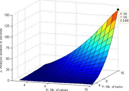
2.2.4 Evaluation with respect to the complexity . . . 43
2.2.5 Evaluation with respect to existing analysis . . . 45
2.3 Measurement-Based Probabilistic Timing Analysis . . . 49
2.3.1 Extreme Value Theory for Timing Analysis . . . 50
2.3.2 Steps in the application of EVT . . . 52
2.3.3 Continuous vs. Discrete Functions . . . 53
2.3.4 Experimental Evaluation . . . 54
2.3.5 Results for Single-Path Programs . . . 55
2.3.6 Results for Multi-Path Programs . . . 59
Introduction
The use of computers to control safety-critical real-time functions has increased rapidly over the past few years. As a consequence, real-time systems — computer systems where the correctness of each computation depends on both the logical re-sults of the computation and the time at which these rere-sults are produced — have become the focus of important study. Since the concept of ”time” is important in real-time application systems, and since these systems typically involve the shar-ing of one or more resources among various contendshar-ing processes, the concept of scheduling is integral to real-time system design and analysis. Scheduling theory, as it pertains to a finite set of requests for resources, is a well-researched topic. However, requests in a real-time environment are often of a recurring nature. Such systems are typically modelled as finite collections of simple, highly repetitive tasks, each of which generates jobs in a predictable manner.
The scheduling algorithm determines which job[s] should be executed at each time-instant. When there is at least one schedule satisfying all constraints of the system, the system is said to be schedulable.
Uniprocessor real-time systems have been well studied since the seminal paper of Liu and Layland [48], which introduces a model of periodic systems. There is a tremendous amount of literature considering scheduling algorithms, feasibility tests and schedulability tests for uniprocessor scheduling. During the last years the real-time systems have evolved to more complex models and architectures. The two main contributions of our work covers these two aspects with results on (probabilistic) models and (multiprocessor) architectures. A real-time model is probabilistic if at least one parameter is described by a random variable.
This document does not contain all our results and it presents a synthesis of the main concepts and the description of the most relevant results. For each contribution we will provide an exhaustive list of our related results and their place in the real-time literature.
The order of the presentation of results is chronological and motivated by how my1 reasoning evolved during this period since my PhD thesis.
My first year working on probabilistic (at ISEP following the suggestion of Prof. Eduardo Tovar) has been spent on understanding how to get closer two worlds that 1This part of the introduction shares with the reader on how I moved from deterministic
seem so different:
• the real-time community imposing worst-case reasoning as basic rule for ob-taining safe results
• the probabilistic community attracted by average behavior of systems and the central part of a distribution describing the parameters.
After publishing a first result on probabilistic [13], I had the conviction that the differences were less important than the misunderstanding surrounding the results on probabilistic but by that time I didn’t have the means to explain what was the misunderstanding. Continuing my visits in Europe, I had started to work on mul-tiprocessor platforms and mainly on the predictability of such platforms (joining Prof. Joel Goossens at ULB). The predictability of an algorithm indicates that any task, that starts earlier and it is shorter than other task, should finish the execution before that latter task. After proving that the first result on predictability had an incorrect proof, we had proposed the most general result (as it was in 2010), here general is defined with respect to the class of scheduling algorithms and architec-tures. Since then, a more general result has been obtained in 2013 in collaboration with J. Goossens and E. Grolleau [35].
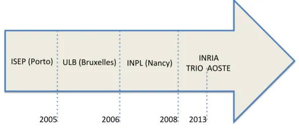
ISEP%(Porto)% ULB%(Bruxelles)% INPL%(Nancy)% INRIA%% TRIO%%AOSTE%
2005% 2006% 2008% 2013%
Figure 1: A timeline
After working at ISEP (Porto) on probabilistic schedulability analysis and at ULB (Bruxelles) on multiprocessor schedulability analysis, I had naturally worked on probabilistic multiprocessor analysis during my first years at INPL (Nancy), where I had joined Prof. F. Simonot-Lion’s team. My first result on this topic [14] has received criticism for the fact that the inputs for such problem (probability dis-tributions for execution times) are impossible to obtain. This feedback had made me realize that no probabilistic schedulability analysis will be understood and accepted by the community as long as no methods for obtaining probability distributions exist. At this point the first Dagstuhl seminar on scheduling (2008) gave me the
opportunity to meet Prof. Alan Burns and this was the event ”provoking” in 2009 my work in the FP7 STREP project PROARTIS. At the end of this project we have proposed several important results that solve partially the problem of obtain-ing probability distributions for probabilistic worst-case execution times [10, 17, 65]. Therefore it is now a good timing to advance on probabilistic schedulability anal-ysis [56] and my unpublished work on probabilistic multiprocessor scheduling [14] will soon meet the appropriate PhD student to become a published paper.
During the first Dagstuhl seminar on scheduling, discussions with Prof. Jane Liu (co-author of one of the first papers on probabilistic real-time systems) made me, also, understand that a second mandatory condition for probabilistic real-time reasoning was to establish the bases of the probabilistic worst-case reasoning. In 2013 I have provided the arguments to sustain the importance of the probabilistic worst-case reasoning and its impact on independence property. These arguments are related to the definition of probabilistic worst-case execution time as it is pro-posed by Edgar and Burns [21]. The paper had propro-posed this new concept without underlining its important impact on imposing a probabilistic worst-case reasoning. Underling this impact is probably the most important contribution of this thesis.
Organization of this document In Chapter 1 we present our contribution to the scheduling of real-time systems on multiprocessor platforms. We start the chapter by providing an exhaustive list of all results we proposed on this topic and then we detail two contributions: the predictability results and the schedulability analysis. We present the proofs of these results as their details are important. The first result on predictability is a corrected and extended version of previous results from [38]. The results on schedulability analysis provide a methodology for feasibility tests based on intervals.
In Chapter 2 we present our contribution to the definition and the analysis of probabilistic real-time systems. We start the chapter by providing an exhaustive list of all results we proposed on this topic and then we detail two contributions. The first contribution concerns the proposition of probabilistic worst-case reason-ing within response time analysis of systems with multiple probabilistic parameters. The second contribution concerns the estimation of probabilistic worst-case execu-tion times and its relaexecu-tion to rare events theory. It indicates that the real-time community should use the mathematical results on the tails of the probability dis-tributions.
In Chapter 3 we present the perspectives of our results and the vision of how these results will modify the real-time community that needs to face data deluge and increased connectivity with less critical systems that will coexist within one larger system built following a mixed-critical model.
Chapter 1
Multiprocessor real-time
systems
This chapter contains results on multiprocessor scheduling of real-time systems. These results are mainly obtained during my stay at Universit´e Libre de Bruxelles in collaboration with Prof. Jo¨el Goossens’s research group.
These results belong to three main classes:
• Predictability of scheduling algorithms on multiprocessor architectures. After proving that previous existing results on predictability for identical platforms was incorrect, we have extended them to the case of unrelated platforms and to a more general class of scheduling algorithms. Our result allows to under-stand the ”mandatory” properties of a scheduling algorithm for multiprocessor architectures and it indicates what algorithms are not predictable.
J1 L. Cucu-Grosjean and J. Goossens, ”Predictability of Fixed-Job Priority Schedulers on Heterogeneous Multiprocessor Real-Time Systems”, Infor-mation Processing Letters 110(10): 399-402, April 2010
O1 E. Grolleau, J. Goossens and L. Cucu-Grosjean, ”On the periodic behavior of real-time schedulers on identical multiprocessor platforms”, arxiv.org, May 2013
The result of this class is published in J1 and it concerns memoryless algo-rithms. This result and the definition of memoryless algorithms are presented in Section 1.1. Recent work allowed us to extend J1 to algorithms that do not have this memoryless constraint in O1.
• Schedulability tests for job-level fixed-priority scheduling algorithms for peri-odic tasks, whatever the type of architecture (identical, uniform or unrelated). These tests were the first exact tests of the real-time literature for such gen-eral architectures. They are based on the construction of feasibility intervals,
that have the existence guaranteed by the periodicity properties of feasible schedules. This methodology was used later by other authors for different real-time multiprocessor scheduling problems (parallel tasks, scheduling sim-ulation, task-level optimal scheduling algorithms, etc).
The following publications belong to this class of results on multiprocessor systems:
J2 L. Cucu-Grosjean and J. Goossens, ”Exact Schedulability Tests for Real-Time Scheduling of Periodic Tasks on Unrelated Multiprocessor Plat-forms”, Journal of System Architecture, 57(5): 561-569, March 2011 C4 B. Miramond and L. Cucu-Grosjean Generation of static tables in
em-bedded memory with dense scheduling, Conference on Design and Archi-tectures for Signal and Image Processing (DASIP), Edinburgh, October 2010
C3 L. Idoumghar, L. Cucu-Grosjean and R. Schott, Tabu Search Type Algo-rithms for the Multiprocessor Scheduling Problem, the 10th IASTED In-ternational Conference on Artificial Intelligence and Applications (AIA), Innsbruck, February 2010
C2 Cucu L. and Goossens, J. ”Feasibility Intervals for Multiprocessor Fixed-Priority Scheduling of Arbitrary Deadline Periodic Systems ”, the 10th Design, Automation and Test in Europe (DATE), ACM Press, Nice, April 2007
C1 Cucu L. and Goossens J., ”Feasibility Intervals for Fixed-Priority Real-Time Scheduling on Uniform Multiprocessors”, the 11th IEEE Interna-tional Conference on Emerging Technologies and Factory Automation, (ETFA), Prague, September 2006
The publication J2 is the most general of this class and it is an extended version of C1 and C2. The content of J2 is detailed in Section 1.2. The conferences publications C4 and C5 make use of the results of J1 in different contexts (C4 for the utilisation of genetic algorithms and C5 for the introduction of memory issues in a multiprocessor context).
• Model of parallel tasks for multiprocessor real-time. Historically, the first models of tasks on multiprocessor architectures forbid the parallelism of tasks without an appropriate justification. In C5 we have provided arguments in favor of parallel tasks and the first model of parallel tasks on identical proces-sors. This model is the starting point of several current results on real-time parallel tasks. The results were published originally in C5 and J3 is an ex-tended version of C5.
J3 Collette S., Cucu L. and Goossens J., ”Integrating job parallelism in real-time scheduling theory”, Information Processing Letters, 106(5): 180-187, May 2008
C5 Collette S., Cucu L. and Goossens, J. ”Algorithm and complexity for the global scheduling of sporadic tasks on multiprocessors with work-limited parallelism”, the 15th International Conference on Real-Time and Net-work systems (RTNS), Nancy, March 2007
Organization of the chapter This chapter has two parts. The first part (within Section 1.1) presents the results on predictability. Most of the proofs are provided as they indicate the misunderstanding within the previous existing proofs. The second part of this chapter (within Section 1.2) collect the main results on feasibility intervals for a large class of scheduling algorithms and architectures.
During this chapter we assume the notions defined below as known.
From a theoretical and a practical point of view, we can distinguish (at least) between three kinds of multiprocessor architectures (from less general to more gen-eral):
Identical parallel machines Platforms on which all processors are identical, in the sense that they have the same computing power.
Uniform parallel machines By contrast, each processor in a uniform parallel machine is characterized by its own computing capacity, a job that is executed on processor ⇡i of computing capacity sifor t time units completes si⇥ t units
of execution.
Unrelated parallel machines In unrelated parallel machines, there is an execu-tion rate si,j associated with each job-processor pair, a job Ji that is executed
on processor ⇡j for t time units completes si,j⇥ t units of execution.
We consider real-time systems that are modeled by set of jobs and implemented upon a platform comprised of several unrelated processors. We assume that the platform
• is fully preemptive: an executing job may be interrupted at any instant in time and have its execution resumed later with no cost or penalty.
• allows global inter-processor migration: a job may begin execution on any processor and a preempted job may resume execution on the same processor as, or a different processor from, the one it had been executing on prior to preemption.
• forbids job parallelism: each job is executing on at most one processor at each instant in time.
The scheduling algorithm determines which job[s] should be executed at each time-instant. Fixed-Job Priority (FJP) schedulers assign priorities to jobs statically and execute the highest-priority jobs on the available processors. Dynamic Priority
(DP) schedulers assign priorities to jobs dynamically (at each instant of time). Pop-ular FJP schedulers include: the Rate Monotonic (RM), the Deadline Monotonic (DM) and the Earliest Deadline First (EDF) [48]. Popular DP schedulers include: the Least Laxity First (LLF) and the EDZL [11, 58].
The specified execution requirement of job is actually an upper bound of its actual value, i.e., the worst case execution time (WCET) is provided. The actual execution requirement may vary depending on the input data, and on the system state (caches, memory, etc.). The schedulability analysis, determining whether all jobs always meet their deadlines, is designed by considering a finite number of (worst-case) scenarios (typically a single scenario) assuming that the scheduler is predictable with the following definition: For a predictable scheduling algorithm, one may determine an upper bound on the completion-times of jobs by analyzing the situation under the assumption that each job executes for an amount equal to the upper bound on its execution requirement; it is guaranteed that the actual completion time of jobs will be no later than this determined value.
1.1
Predictability of Fixed-Job Priority Schedulers
on Heterogeneous Multiprocessor Real-Time
Sys-tems
The results presented in this section were published in [15].
In this section we extend and correct [38] by considering unrelated multipro-cessor platforms and by showing that any FJP schedulers are predictable on these platforms. Ha and Liu [38] ”showed” that FJP schedulers are predictable on iden-tical multiprocessor platforms. However, while the result is correct, an argument used in the proof is not. Han and Park studied the predictability of the LLF sched-uler for identical multiprocessors [39]. To the best of our knowledge a single work addressed heterogeneous architectures, indeed we have showed in [12] that any FJP schedulers are predictable on uniform multiprocessors.
1.1.1
Definitions and assumptions
Within Section 1.1 we consider that a real-time system is modelled as a finite col-lection of independent recurring tasks, each of which generates a potentially infinite sequence of jobs. Every job is characterized by a 3-tuple (ri, ei, di), i.e., by a release
time (ri), an execution requirement (ei), and a deadline (di), and it is required that
a job completes execution between its arrival time and its deadline.
We consider multiprocessor platforms ⇡ composed of m unrelated processors: {⇡1, ⇡2, . . . , ⇡m}. Execution rates si,j are associated with each job-processor pair, a
job Ji that is executed on processor ⇡j for t time units completes si,j ⇥ t units of
execution. For each job Ji we assume that the associated set of processors ⇡ni,1 > ⇡ni,2 >· · · > ⇡ni,m are ordered in a decreasing order of the execution rates relative
to the job: si,ni,1 ≥ si,ni,2 ≥ · · · ≥ si,ni,m. For identical execution rates, the ties are broken arbitrarily, but consistently, such that the set of processors associated with each job is totally ordered. For the processor-job pair (⇡j, Ji) if si,j 6= 0 then ⇡j is
said to be an eligible processor for Ji.
Definition 1 (Schedule σ(t)). For any set of jobs J def= {J1, J2, J3, . . .} and any set
of m processors {⇡1, . . . , ⇡m} we define the schedule σ(t) of system ⌧ at time-instant
t as σ : N! Nm where σ(t)def= (σ 1(t), σ2(t), . . . , σm(t)) with σj(t) def = ⇢
0, if there is no job scheduled on ⇡jat time-instant t;
i, if job Ji is scheduled on ⇡j at time-instant t.
Definition 2 (Work-conserving algorithm). An unrelated multiprocessor scheduling algorithm is said to be work-conserving if, at each instant, the algorithm schedules jobs on processors as follows: the highest priority (active) job Ji is scheduled on
its fastest (and eligible) processor ⇡j. The very same rule is then applied to the
remaining active jobs on the remaining available processors.
Throughout this paper, J denotes a (finite or infinite) set of jobs: J def= {J1, J2, J3, . . .}.
We consider any FJP scheduler and without loss of generality we consider jobs in a decreasing order of priorities (J1 > J2 > J3 > · · · ). We suppose that the actual
execution time of each job Ji can be any value in the interval [e−i , e+i ] and we denote
by Ji+the job defined as Ji+ def= (ri, e+i , di). The associated execution rates of Ji+ are
s+i,j def= si,j,8j. Similarly, Ji− is the job defined from Ji as follows: Ji− = (ri, e−i , di).
Similarly, the associated execution rates of Ji− are s−i,j def= si,j,8j. We denote by
J(i) the set of the i highest priority jobs (and its schedule by σ(i)). We denote also by J−(i) the set {J1−, . . . , J
−
i } and by J (i)
+ the set {J1+, . . . , Ji+} (and its schedule by
σ(i)+ ). Note that the schedule of an ordered set of jobs using a work-conserving and FJP scheduler is unique. Let S(J) be the time-instant at which the lowest priority job of J begins its execution in the schedule. Similarly, let F (J) be the time-instant at which the lowest priority job of J completes its execution in the schedule.
Definition 3 (Predictable algorithm). A scheduling algorithm is said to be pre-dictable if S(J−(i)) S(J(i)) S(J
(i) + ) and F (J (i) − ) F (J(i)) F (J (i) + ), for all
1 i #J and for all schedulable J+(i) sets of jobs.
Definition 4 (Availability of the processors). For any ordered set of jobs J and any set of m unrelated processors {⇡1, . . . , ⇡m}, we define the availability of the
proces-sors A(J, t) of the set of jobs J at time-instant t as the set of available procesproces-sors: A(J, t)def= {j | σj(t) = 0} ✓ {1, . . . , m}, where σ is the schedule of J.
1.1.2
Proof from Ha and Liu [38]
Theorem 5. For any FJP scheduler and identical multiprocessor platform, the start time of every job is predictable, that is, S(J−(i)) S(J(i)) S(J
(i) + ).
We give here the first part of the original (adapted with our notations) proof of Ha and Liu, Theorem 3.1, page 165 of [38].
Proof from [38]. Clearly, S(J(1)) S(J+(1)) is true for the highest-priority job J1. Assuming that S(J(k)) S(J+(k)) for k < i, we now prove S(J(i)) S(J
(i) + ) by
contradiction. Suppose S(J(i)) > S(J+(i)). Because we consider a FJP scheduler, every job whose release time is at or earlier than S(J+(i)) and whose priority is higher than Ji has started by S(J+(i)) according to the maximal schedule σ
(i)
+ . From the
induction hypothesis, we can conclude that every such job has started by S(J+(i)) in the actual schedule σ(i). Because ek e+k for all k, in (0, S(J+(i))), the total demand
of all jobs with priorities higher than Ji in the maximal schedule σ+(i) is larger than
the total time demand of these jobs in the actual schedule σ(i). In σ+(i), a processor is available at S(J+(i)) for Ji to start; a processor must also be available in σ(i) at or
before S(J+(i)) on which Ji or a lower-priority job can be scheduled.
Counter-example. The use of the notion of “total demand” used in the original proof is not appropriate considering multiprocessor platforms. Consider, for in-stance, two set of jobs: J def= {J1 = J2 = (0, 3,1)} and J0 def= {J3 = (1, 5,1), J4 =
(1, 1,1)}. In (0, 2) the total demands of both job sets are identical (i.e., 6 time units), if we schedule the system using FJP schedulers, e.g., J1 > J2 and J3 > J4
it is not difficult to see that in the schedule of J0 a processor is available at time 2 while in the schedule of J we have to wait till time-instant 3 to have available processor(s).
1.1.3
Predictability
In this section we prove our main property, the predictability of FJP schedulers on unrelated multiprocessors which is based on the following lemma.
Lemma 1.1.1. For any schedulable ordered set of jobs J (using a FJP and work-conserving scheduler) on an arbitrary set of unrelated processors {⇡1, . . . , ⇡m}, we
have A(J+(i), t) ✓ A(J(i), t), for all t and all i. In other words, at any time-instant
the processors available in σ+(i) are also available in σ(i). (We consider that the sets
of jobs are ordered in the same decreasing order of the priorities, i.e., J1 > J2 >
· · · > J` and J1+> J2+ >· · · > J`+.)
Proof. The proof is made by induction by ` (the number of jobs). Our inductive hypothesis is the following: A(J+(k), t) ✓ A(J(k), t), for all t and 1 k i.
The property is true in the base case since A(J+(1), t) ✓ A(J(1), t), for all t.
Indeed, S(J(1)) = S(J+(1)). Moreover J1 and J1+ are both scheduled on their fastest
(same) processor ⇡n1,1, but J
+
1 will be executed for the same or a greater amount
of time than J1.
We will show now that A(J+(i+1), t) ✓ A(J(i+1), t), for all t.
Since the jobs in J(i) have higher priority than Ji+1, then the scheduling of
Ji+1 will not interfere with higher priority jobs which have already been scheduled.
Similarly, Ji+1+ will not interfere with higher priority jobs of J+(i) which have already been scheduled. Therefore, we may build the schedule σ(i+1) from σ(i), such that the jobs J1, J2, . . . , Ji, are scheduled at the very same instants and on the very same
processors as they were in σ(i). Similarly, we may build σ(i+1)+ from σ+(i).
Note that A(J(i+1), t) will contain the same available processors as A(J(i), t) for all t except the time-instants at which J(i+1) is scheduled, and similarly A(J+(i+1), t) will contain the same available processors as A(J+(i), t) for all t except the time-instants at which J+(i+1) is scheduled. From the inductive hypothesis we have A(J+(i), t) ✓ A(J(i), t), we will consider time-instant t, from r
i+1 to the
comple-tion of Ji+1 (which is actually not after the completion of Ji+1+ , see below for a
proof), we distinguish between four cases:
1. A(J(i), t) = A(J+(i), t) = 0: in both situations no processor is available. There-fore, both jobs, Ji+1 and Ji+1+ , do not progress and we obtain A(J(i+1), t) =
A(J+(i+1), t). The progression of Ji+1 is identical to Ji+1+ .
2. A(J(i), t) 6= ; and A(J+(i), t) = ;: if an eligible processor exists, Ji+1 progress
on an available processor in A(J(i), t) not available in A(J+(i), t), Ji+1+ does not progress. Consequently, A(J+(i+1), t)✓ A(J(i+1), t) and the progression of J
i+1
is strictly larger than Ji+1+ .
3. A(J(i), t) = A(J+(i), t) 6= ;: if an eligible processor exists, Ji+1 and Ji+1+
progress on the same processor. Consequently, A(J+(i+1), t) = A(J(i+1), t) and
the progression of Ji+1 is identical to Ji+1+ .
4. A(J(i), t) 6= A(J(i)
+ , t) 6= ;: if the faster processor in A(J(i), t) and A(J (i) + , t)
is the same see previous case of the proof (case 3); otherwise Ji+1 progress
on a faster processor than Ji+1+ , that processor is not available in A(J+(i), t), consequently a slower processor remains idle in A(J(i), t) but busy in A(J+(i), t). Consequently, A(J+(i+1), t) ✓ A(J(i+1), t) and the progression of J
i+1 is larger
than Ji+1+ .
Therefore, we showed that A(J+(i+1), t)✓ A(J(i+1), t)8t, from r
i+1to the completion
of Ji+1 and that Ji+1 does not complete after Ji+1+ . For the time-instant after the
Theorem 6. FJP schedulers are predictable on unrelated platforms.
Proof. In the framework of the proof of Lemma 1.1.1 we actually showed extra properties which imply that FJP schedulers are predictable on unrelated platforms: (i) Ji+1 completes not after Ji+1+ and (ii) Ji+1 can be scheduled either at the very
same instants as Ji+1+ or may progress during additional time-instants (case (2) of the proof) these instants may precede the time-instant where Ji+1+ commences its execution.
Since multiprocessor real-time scheduling researchers pay attention to uniform platforms (at least nowadays), we find convenient to emphasize the following corol-lary:
Corollary 7. FJP schedulers are predictable on uniform platforms.
1.2
Exact Schedulability Tests for Periodic Tasks on
Unrelated Multiprocessor Platforms
The results presented in this section were published in [16].
In this section, we study the global scheduling of periodic task systems on un-related multiprocessor platforms. We first show two general properties which are well-known for uniprocessor platforms and which are also true for unrelated mul-tiprocessor platforms: (i) under few and not so restrictive assumptions, we prove that feasible schedules of periodic task systems are periodic starting from some point in time with a period equal to the least common multiple of the task periods and (ii) for the specific case of synchronous periodic task systems, we prove that feasible schedules repeat from their origin. We then characterize, for task-level fixed-priority schedulers and for asynchronous constrained or arbitrary deadline periodic task models, upper bounds of the first time-instant where the schedule repeats. For task-level fixed-priority schedulers, based on the upper bounds and the predictabil-ity property, we provide exact schedulabilpredictabil-ity tests for asynchronous constrained or arbitrary deadline periodic task sets.
The problem of scheduling periodic task systems on multiprocessors was origi-nally studied in [47]. Recent studies provide a better understanding of this schedul-ing problem and provide the first solutions, e.g., [9] presents a categorization of real-time multiprocessor scheduling problems and [19] an up-to-date state of the art. To the best of our knowledge, a single work [5] provides exact schedulability tests for the global scheduling of periodic systems on multiprocessors. Baker and Cirinei present a test for global preemptive priority-based scheduling of sporadic tasks on identical processors. Our work differs for several reasons: (i) we extend the model by considering unrelated platforms, and (ii) we provide a schedulability interval and the periodic characterization of the schedule. Such characterization is not straightforward since we know that not all uniprocessor schedulability results
or arguments are true for multiprocessor scheduling. For instance, the synchronous case (i.e., considering that all tasks start their execution synchronously) is not the worst case on multiprocessors anymore [33]. Another example is the fact that the first busy period (see [45] for details) does not provide a schedulability interval on multiprocessors (see [33] for such counter-examples). By schedulability interval we mean a finite interval such that, if no deadline is missed while only considering requests within this interval then no deadline will ever be missed.
The tests that we present have, for a set of n tasks, a time complexityO(lcm{T1,
T2, . . . , Tn}), which is unfortunately also the case of most schedulability tests for
simpler uni processor scheduling problems.
1.2.1
Definitions and assumptions
We consider the preemptive global scheduling of periodic task systems. A system ⌧ is composed of n periodic tasks ⌧1, ⌧2, . . . , ⌧n, where each task is characterized by
a period Ti, a relative deadline Di, an execution requirement Ci and an offset Oi.
Such a periodic task generates an infinite sequence of jobs, with the kth job arriving
at time-instant Oi+ (k− 1)Ti (k = 1, 2, . . .), having an execution requirement of Ci
units, and a deadline at time-instant Oi+ (k−1)Ti+ Di. It is important to note that
we assume first that each job of the same task ⌧ihas the same execution requirement
Ci; we relax this assumption then by showing that our analysis is robust.
We will distinguish between implicit deadline systems where Di = Ti,8i;
con-strained deadline systems where Di Ti,8i and arbitrary deadline systems where
there is no relation between the deadlines and the periods.
In some cases, we will consider the more general problem of scheduling a set of jobs, each job Jj is characterized by a release time rj, an execution requirement ej
and an absolute deadline dj. The job Jj must execute for ej time units over the
interval [rj, dj). A job becomes active from its release time to its completion.
A periodic system is said to be synchronous if there is a time-instant where all tasks make a new request simultaneously, i.e., 9t, k1, k2, . . . kn such that 8i : t =
Oi+ kiTi(see [30] for details). Without loss of generality, we consider Oi = 0,8i for
synchronous systems. Otherwise the system is said to be asynchronous. We denote by ⌧(i) def= {⌧1, . . . , ⌧i}, by Oimax
def
= max{O1, . . . , Oi}, by Omax def=
On max, by P0 def= 0, Pi def = lcm{T1, . . . , Ti} (0 < i n) and by P def = Pn. In the
following, the quantity P is called the task set hyper-period.
We consider multiprocessor platforms ⇡ composed of m unrelated processors (or one of its particular cases: uniform and identical platforms): {⇡1, ⇡2, . . . , ⇡m}.
Execution rates si,j are associated with each task-processor pair. A task ⌧i that
is executed on processor ⇡j for t time units completes si,j ⇥ t units of execution.
For each task ⌧i we assume that the associated set of processors ⇡ni,1 > ⇡ni,2 > · · · > ⇡ni,m are ordered in a decreasing order of the execution rates relative to the task: si,ni,1 ≥ si,ni,2 ≥ · · · ≥ si,ni,m. For identical execution rates, the ties are broken arbitrarily, but consistently, such that the set of processors associated with each task
is totally ordered. Consequently, the fastest processor relative to task ⌧i is ⇡ni,1, i.e., the first processor of the ordered set associated with the task. Moreover, for a task ⌧i in the following we consider that a processor ⇡a is faster than ⇡b (relative
to its associated set of processors) if ⇡a > ⇡b even if we have si,a = si,b. For the
processor-task pair (⇡j, ⌧i) if si,j 6= 0 then ⇡j is said to be an eligible processor for ⌧i.
Note that these concepts and definitions can be trivially adapted to the scheduling of jobs on unrelated platforms.
In this work we consider a discrete model, i.e., the characteristics of the tasks and the time are integers. Moreover, in the following we will illustrate main concepts and definitions using the following system.
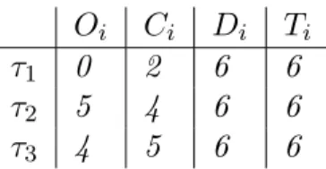
Example 1. Let ⌧ be a system of three periodic tasks
Oi Ci Di Ti
⌧1 0 2 6 6
⌧2 5 4 6 6
⌧3 4 5 7 6
Let ⇡ be a multiprocessor platform of 2 unrelated processors ⇡1 and ⇡2. We have
s1,1= 1, s1,2= 2, s2,1= 2, s2,2= 1, s3,1= 2 and s3,2 = 1. Note that according to our
definition above and regarding task ⌧1 we have that ⇡2 > ⇡1.
The notions of the state of the system and the schedule are as follows.
Definition 1 (State of the system ✓(t)). For any arbitrary deadline task system ⌧ = {⌧1, . . . , ⌧n} we define the state ✓(t) of the system ⌧ at time-instant t as ✓ :
N ! (Z ⇥ N ⇥ N)n with ✓(t)def= (✓ 1(t), ✓2(t), . . . , ✓n(t)) where ✓i(t)def= 8 > > > > > > > > > > > > < > > > > > > > > > > > > :
(−1, x, 0), if no job of task ⌧i was activated before or at t. In this
case, x time units remain until the first activation of ⌧i. We have 0 < x Oi.
(y, z, u), otherwise. In this case, y denotes the number of active jobs of ⌧i at t, z denotes the time elapsed at
time-instant t since the arrival of the oldest active job of ⌧i, and u denotes the amount that the oldest active job
has executed for. If there is no active job of ⌧i at t,
then u is 0.
Note that at any time-instant t several jobs of the same task might be active and we consider that the oldest job is scheduled first, i.e., the FIFO rule is used to serve the various jobs of a given task.
Definition 2 (Schedule σ(t)). For any task system ⌧ = {⌧1, . . . , ⌧n} and any set of
as σ : N! {0, 1, . . . , n}m where σ(t)def= (σ 1(t), σ2(t), . . . , σm(t)) with σj(t) def = 8 < :
0, if there is no task scheduled on ⇡j
at time-instant t;
i, if task ⌧i is scheduled on ⇡j at time-instant t.
81 j m.
A system ⌧ is said to be schedulable on a multiprocessor platform if there is at least one feasible schedule, i.e., a schedule in which all tasks meet their deadlines. If A is an algorithm which schedules ⌧ on a multiprocessor platform to meet its deadlines, then the system ⌧ is said to be A-schedulable.
Note that for a feasible schedule from Definition 1 we have 0 y dDi
Tie, 0 z < Ti· dDTiie and 0 u < Ci.
The scheduling algorithms considered in this paper are work-conserving (see Definition 2) and deterministic with the following definition:
Definition 3 (Deterministic algorithm). A scheduling algorithm is said to be de-terministic if it generates a unique schedule for any given set of jobs.
Note that we assume in this work that no two jobs/tasks share the same priority. It follows by Definition 2 that a processor ⇡j can be idle and a job Ji can be active
at the same time if and only if si,j = 0.
Moreover, we will assume that the decision of the scheduling algorithm at time t is not based on the past, nor on the actual time t, but only on the characteristics of active tasks and on the state of the system at time t. More formally, we consider memoryless schedulers.
Definition 4 (Memoryless algorithm). A scheduling algorithm is said to be memo-ryless if the scheduling decision it made at time t depends only on the characteristics of active tasks and on the current state of the system, i.e., on ✓(t).
Consequently, for memoryless and deterministic schedulers we have the following property:
8t1, t2 such that ✓(t1) = ✓(t2) then σ(t1) = σ(t2).
Note that popular real-time schedulers, e.g., EDF and Deadline Monotonic (DM), are memoryless: the priority of each task is only based on its absolute (EDF) or relative (DM) deadline.
In the following, we will distinguish between two kinds of schedulers:
Definition 5 (Task-level fixed-priority). A scheduling algorithm is a task-level fixed-priority algorithm if it assigns the priorities to the tasks beforehand; at run-time each job priority corresponds to its task priority.
Definition 6 (Job-level priority). A scheduling algorithm is a job-level fixed-priority algorithm if and only if it satisfies the condition that: for every pair of jobs Ji and Jj, if Ji has higher priority than Jj at some time-instant, then Ji always has
Popular task-level fixed-priority schedulers include the RM and the DM al-gorithms; popular job-level fixed-priority schedulers include the EDF algorithm, see [48] for details.
Definition 7 (Job Jk
i of a task ⌧i). For any task ⌧i, we define Jik to be the k th
job of task ⌧i, which becomes active at time-instant Rki
def
= Oi+ (k− 1)Ti. For two tasks
⌧i and ⌧j, by Jik > Jj` we mean that the job Jik has a higher priority than the job Jj`.
Definition 8 (Executed time ✏k
i(t) for a job Jik). For any task ⌧i, we define ✏ki(t)
to be the amount of time already executed for Jk
i in the interval [Rki, t).
We now introduce the availability of the processors for any schedule σ(t).
Definition 9 (Availability of the processors a(t)). For any task system ⌧ ={⌧1, . . . , ⌧n}
and any set of m processors {⇡1, . . . , ⇡m} we define the availability of the processors
a(t) of system ⌧ at time-instant t as the set of available processors a(t) def= {j | σj(t) = 0} ✓ {1, . . . , m}.
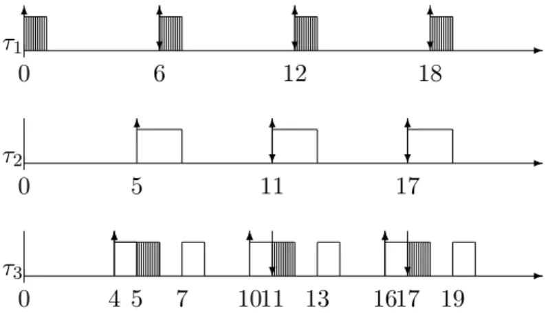
In Example 1 for a preemptive task-level fixed-priority algorithm with ⌧1 the
highest priority task and ⌧3 the lowest priority task, we obtain the schedule provided
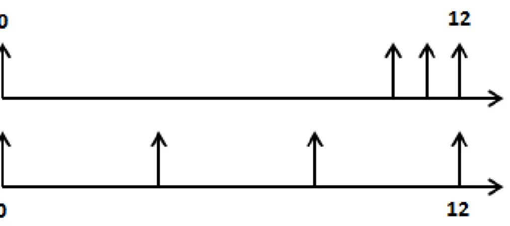
in Figure 1.1. In this figure the execution on the first processor is indicated by black boxes. The releases of jobs are indicated by " and the deadlines by #.
For instance we have ✓2(2) = (−1, 3, 0), ✓1(3) = (3, 0, 0) and ✓3(6) = (2, 1, 3).
Moreover σ(6) = (2, 1) and σ(7) = (3, 0). Concerning task ⌧1, its job J12 becomes
active at R2
1 = 6 and this job has a higher priority than the job J21 of task ⌧2. For
this schedule a(1) ={1} and a(6) = ;.
-0 4 5 7 1011 13 1617 19 -0 5 11 17 -0 6 12 18 ⌧3 ⌧2 ⌧1 6 6 6 6 6 6 6 6 6 6 6 6 6 ? ? ? ? ? ? ?
Figure 1.1: Schedule (obtained using a task-level fixed-priority scheduling) for the task set of Example 1
1.2.2
Periodicity of feasible schedules
We assume in this section that each job of the same task ⌧i has the same execution
requirement Ci. We will relax this assumption in Section 1.2.3.
This section contains four parts. In each part of this section we give results concerning the periodicity of feasible schedules. By periodicity (assuming that the period is γ) of a schedule σ, we mean there is a time-instant t0 and an interval
length γ such that σ(t) = σ(t + γ),8t ≥ t0. For instance, in Figure 1.1 the schedule
is periodic from t = 5 with a period equal to 6.
The first part of this section provides periodicity results for a general scheduling algorithm class: deterministic, memoryless and work-conserving schedulers. The second part of this section provides periodicity results for synchronous periodic task systems. The third and the fourth parts of this section present periodicity results for task-level fixed-priority scheduling algorithms for constrained and arbitrary deadline systems, respectively.
Periodicity of deterministic, memoryless and work-conserving scheduling algorithms
We show that feasible schedules of periodic task systems obtained using determin-istic, memoryless and work-conserving algorithms are periodic starting from some point. Moreover, we prove that the schedule repeats with a period equal to P for a sub-class of such schedulers. Based on that property, we provide two interesting corollaries for preemptive task-level fixed-priority algorithms (Corollary 1) and for preemptive deterministic EDF 1 (Corollary 2).
We first present two basic results in order to prove Theorem 1.
Lemma 1. For any deterministic and memoryless algorithm A, if an asynchronous arbitrary deadline system ⌧ is A-schedulable on m unrelated processor platform ⇡, then the feasible schedule of ⌧ on ⇡ obtained using A is periodic with a period di-visible by P .
Proof. First note that from any time instant t0 ≥ Omax all tasks are released,
and the configuration ✓i(t0) of each task is a triple of finite integers (↵, β, γ) with
↵ 2 {0, 1, . . . , dDi
Tie}, 0 β < max1in(Ti ⇥ d
Di
Tie) and 0 γ < max1inCi. Therefore, there is a finite number of different system states, hence we can find two distinct instants t1 and t2 (t2 > t1 ≥ t0) with the same state of the system
(✓(t1) = ✓(t2)). The schedule repeats from that instant with a period dividing
t2− t1, since the scheduler is deterministic and memoryless.
Note that, since the tasks are periodic, the arrival pattern of jobs repeats with a period equal to P from Omax.
We now prove by contradiction that t2− t1 is necessarily a multiple of P . We
suppose that 9k1 < k2 2 N such that ti = Omax + kiP + ∆i,8i 2 {1, 2} with
∆1 6= ∆2, ∆1, ∆2 2 [0, P ) and ✓(t1) = ✓(t2). This implies that there are tasks for
which the time elapsed since the last activation at t1 and the time elapsed since
the last activation at t2 are not equal. But this is in contradiction with the fact
that ✓(t1) = ✓(t2). Consequently, ∆1 must be equal to ∆2 and, thus, we have
t2− t1 = (k2− k1)P .
For a sub-class of schedulers, we will show that the period of the schedule is P and we provide first a definition (inspired from [32]):
Definition 10 (Request-dependent scheduler). A scheduler is said to be request-dependent when 8i, j, k, ` : Jk+hi
i > J `+hj
j if and only if Jik > Jj`, where hi def
= TPi.
Note that Definition 10 (request-dependent) is stronger than Definition 6 (job-level fixed-priority) ; informally speaking Definition 10 requires that the same total order is used each hyper-period between “corresponding” jobs (Jk
i “corresponds” to
Jk+hi
i ). For instance in Example 1 for the schedule of Figure 1.1 we have J11 > J21
and J13 > J23 because the hyper-period is 6.
The next lemma extends results given for arbitrary deadline task systems in the uniprocessor case (see [29], p. 55 for details).
Lemma 2. For any preemptive, job-level fixed-priority and request-dependent al-gorithm A and any asynchronous arbitrary deadline system ⌧ on m unrelated pro-cessors, we have: for each task ⌧i, for any time-instant t ≥ Omax and k such
that Rk
i t Rik + Di, if there is no deadline missed up to time t + P , then
✏k
i(t)≥ ✏k+hi i(t + P ) with hi def
= TP i. Proof. Note first that the function ✏k
i(·) is a non-decreasing discrete2 step function
with 0 ✏k i(t) Ci,8t and ✏ki(Rki) = 0 = ✏ k+hi i (R k+hi i ),8k.
Note, also that, since the tasks are periodic, the arrival pattern of jobs repeats with a period equal to P from Omax.
The proof is made by contradiction. Thus, we assume that a first time-instant t exists such that there are j and k with Rkj t Rk
j + Dj and ✏kj(t) < ✏ k+hj
j (t + P ).
This assumption implies that:
1. either there is a time-instant t0 with Rk
j t0< t such that J k+hj
j is scheduled
at t0+P while Jk
j is not scheduled at t
0. We obtain that there is at least one job
Jk`+h`
` of a task ⌧` with `2 {1, 2, . . . , n} that is not scheduled at t
0+ P , while Jk` ` is scheduled at t 0 (h` def = TP
`). This implies (since the tasks are scheduled according to a request-dependent algorithm, the arrival pattern of jobs repeats with a period equal to P from Omax and there is no deadline missed) that J`k`
has not finished its execution before t0, but Jk`+h`
` has finished its execution
2We assume that the time unit chosen is small enough such that all execution
before t0+ P . Therefore, we have ✏k`+h`
` (t
0
+ P ) = C`, which implies that
✏k` ` (t 0 ) < ✏k`+h` ` (t 0
+ P ). This last relation is in contradiction with the fact that t is the first such time instant.
2. or there is at least one time-instant t00+P < t+P when Jk+hj
j is scheduled on a
faster processor than the processor on which Jk
j is scheduled at t00. This implies
(since the tasks are scheduled according to a request-dependent algorithm) that there is, at least, one job Jk`+h`
` of a task ⌧` with `2 {1, 2, . . . , n} that is
not scheduled at t00+ P , while Jk`
` is scheduled at t 00 (h ` def = TP `). As proved in the first case, this situation leads us to a contradiction with our assumption.
For the task set of Example 1 and the schedule of Figure 1.1, we have from Lemma 2 that for t = 6 and k = 1, ✏1
3(6) = 3 = ✏23(12) and no deadline missed up
to 12.
Theorem 1. For any preemptive job-level fixed-priority and request-dependent al-gorithm A and any A-schedulable asynchronous arbitrary deadline system ⌧ on m unrelated processors the schedule is periodic with a period equal to P .
Proof. By Lemma 1 we have 9ti = Omax + kiP + d,8i 2 {1, 2} with 0 d < P
such that ✓(t1) = ✓(t2). We know also that the arrivals of task jobs repeat with a
period equal to P from Omax. Therefore, for all time-instants t1+ kP , 8k < k2− k1
(i.e. t1+ kP < t2), the time elapsed since the last activation at t1+ kP is the same
for all tasks. Moreover since ✓(t1) = ✓(t2) we have ✏`ii(t1) = ✏
`i+(k2−k1)PTi
i (t2) with
`i def= dt1−OTi ie, 8i. But by Lemma 2 we also have ✏`ii(t1) ≥ ✏ `i+TiP
i (t1+ P ) ≥ · · · ≥
✏`i+
(k2−k1)P Ti
i (t2),8i. Consequently we obtain ✓(t1) ≥ ✓(t1 + P ) ≥ · · · ≥ ✓(t2) and
✓(t1) = ✓(t2) which 3 implies that ✓(t1) = ✓(t1+ P ) =· · · = ✓(t2).
Corollary 1. For any preemptive task-level fixed-priority algorithm A, if an asyn-chronous arbitrary deadline system ⌧ is A-schedulable on m unrelated processors, then the schedule is periodic with a period equal to P .
Proof. The result is a direct consequence of Theorem 1, since task-level fixed-priority algorithms are job-level fixed-priority and request-dependent schedulers.
Corollary 2. A feasible schedule obtained using deterministic request-dependent global EDF on m unrelated processors of an asynchronous arbitrary deadline system ⌧ is periodic with a period equal to P .
3where θ(t) ≥ θ(t0) means that, for each task, the system state at time t and t0 are identical
regarding n1 and t2, moreover if n1 >0 we must have that the time elapsed for the oldest active
request of the task at time t is not shorter than the time elapsed for the oldest active request of the task at time t0.
Proof. The result is a direct consequence of Theorem 1, since EDF is a job-level fixed-priority scheduler.
The particular case of synchronous arbitrary deadline periodic systems In this section, we deal with the periodicity of feasible schedules of synchronous arbitrary deadline periodic systems. Using the results obtained for deterministic, memoryless and work-conserving algorithms, we study synchronous arbitrary dead-line periodic systems and the periodicity of feasible schedules of these systems under preemptive task-level fixed-priority scheduling algorithms.
In the following, and without loss of generality, we consider the tasks ordered in decreasing order of their priorities ⌧1 > ⌧2 >· · · > ⌧n.
Lemma 3. For any preemptive task-level fixed-priority algorithm A and for any synchronous arbitrary deadline system ⌧ on m unrelated processors, if no deadline is missed in the time interval [0, P ) and if ✓(0) = ✓(P ), then the schedule of ⌧ is periodic with a period P that begins at time-instant 0.
Proof. Since at time-instants 0 and P the system is in the same state, i.e. ✓(0) = ✓(P ), then at time-instants 0 and P a preemptive task-level fixed-priority algorithm will make the same scheduling decision and the scheduled repeats from 0 with a period equal to P .
Theorem 2. For any preemptive task-level fixed-priority algorithm A and any syn-chronous arbitrary deadline system ⌧ on m unrelated processors, if all deadlines are met in [0, P ) and ✓(0)6= ✓(P ), then ⌧ is not A-schedulable.
Proof. The proof is provided in [16].
Corollary 3. For any preemptive task-level fixed-priority algorithm A and any synchronous arbitrary deadline system ⌧ on m unrelated processors, if ⌧ is A-schedulable, then the schedule of ⌧ obtained using A is periodic with a period P that begins at time-instant 0.
Proof. Since ⌧ is A-schedulable, we know by Theorem 2 that ✓(0) = ✓(P ). Moreover, a deterministic and memoryless scheduling algorithm will make the same scheduling decision at those instants. Consequently, the schedule repeats from its origin with a period of P .
Task-level fixed-priority scheduling of asynchronous constrained deadline systems
In this section we describe another important result: any feasible schedule on m unrelated processors of asynchronous constrained deadline systems, obtained using preemptive task-level fixed-priority algorithms, is periodic from some point (Theo-rem 3) and we characterize that point.
Without loss of generality, we consider the tasks ordered in a decreasing order of their priorities ⌧1> ⌧2 >· · · > ⌧n.
Theorem 3. For any preemptive task-level fixed-priority algorithm A and any A-schedulable asynchronous constrained deadline system ⌧ on m unrelated processors, the schedule is periodic with a period Pn from time-instant Sn where Si is defined
inductively as follows:
• S1 def= O1;
• Si def
= max{Oi, Oi+dSi−1T−Oi ieTi}, 8i 2 {2, 3, . . . , n}.
Proof. The proof is provided in [16].
Example 2. Let ⌧ be a system of three periodic tasks
Oi Ci Di Ti
⌧1 0 2 6 6
⌧2 5 4 6 6
⌧3 4 5 6 6
Let ⇡ be a multiprocessor platform of 2 unrelated processors ⇡1 and ⇡2. We have
s1,1= 1, s1,2= 2, s2,1= 2, s2,2= 1, s3,1= 2 and s3,2 = 1.
Using a task-level fixed-priority scheduling algorithm with ⌧1 the highest priority,
we obtain the schedule provided in Figure 1.2. For this schedule and the notations of Theorem 3, we have S1 = 0, S2 = 5 and S3 = 10. In Figure 1.2 the execution on
the first processor is indicated by black boxes.
-0 4 5 7 1011 13 1617 19 -0 5 11 17 -0 6 12 18 ⌧3 ⌧2 ⌧1 6 6 6 6 6 6 6 6 6 6 6 6 6 ? ? ? ? ? ? ?
Figure 1.2: Schedule (obtained using a task-level fixed-priority scheduling) for the task set of Example 2
Task-level fixed-priority scheduling of asynchronous arbitrary deadline systems
In this section we present another important result: any feasible schedule on m unrelated processors of asynchronous arbitrary deadline systems, obtained using preemptive task-level fixed-priority algorithms, is periodic from some point (Theo-rem 4).
Corollary 4. For any preemptive task-level fixed-priority algorithm A and any asyn-chronous arbitrary deadline system ⌧ on m unrelated processors, we have: for each task ⌧i, for any time-instant t ≥ Oi and k such that Rki t Rki + Di, if there is
no deadline missed up to time t + P , then ✏ki(t) ≥ ✏k+hi
i (t + P ) with hi def
= TP i. Proof. This result is a direct consequence of Lemma 2 since preemptive task-level fixed-priority algorithms are job-level fixed-priority and request-dependent sched-ulers.
In the following corollary we use the notation ✓i(t) = (↵i(t), βi(t), γi(t)),8⌧i.
Corollary 5. For any preemptive task-level fixed-priority algorithm A and any asyn-chronous arbitrary deadline system ⌧ on m unrelated processors, we have: for each task ⌧i, for any time-instant t ≥ Oimax, if there is no deadline missed up to time
t + P , then either (↵i(t) < ↵i(t + P )) or [↵i(t) = ↵i(t + P ) and γi(t)≥ γi(t + P )].
Proof. The proof is provided in [16].
Lemma 4. For any preemptive task-level fixed-priority algorithm A and any A-schedulable asynchronous arbitrary deadline system ⌧ of n tasks on m unrelated processors, let σ(i) the schedule obtained by considering only the task subset ⌧(i). Moreover, let the set of { bS1,· · · , bSn} be defined inductively as follows:
• bS1 def= O1 • bSi def = max{Oi, Oi+d b Si−1−Oi Ti eTi} + Pi, (i > 1)
If ✓i+1( bSi+1) 6= ✓i+1( bSi+1+ Pi+1), then @t 2 [ bSi+1, bSi+1 + Pi+1) such that at t
there is at least one available (and eligible) processor for ⌧i+1 in σ(i) and no job of
⌧i+1 is scheduled at t in σ(i+1).
Proof. The proof is made by contradiction and it is provided in [16].
Theorem 4. For any preemptive task-level fixed-priority algorithm A and any A-schedulable asynchronous arbitrary deadline system ⌧ on m unrelated processors, the schedule is periodic with a period Pn from time-instant bSn where bSn are defined
inductively as follows:
• bSi def= max{Oi, Oi+d b Si−1−Oi
Ti eTi} + Pi, (i > 1)
Proof. The proof is made by induction and it is provided in [16].
1.2.3
Exact schedulability tests
In the previous sections, we assumed that the execution requirement of each task is constant while the designer actually only knows an upper bound on the actual execution requirement, i.e., the worst case execution time (WCET). Consequently, we need tests that are robust relatively to the variation of the execution times up to a worst case value. More precisely, we need predictable schedulers on the considered platforms.
In order to provide exact schedulability tests for various kind schedulers and platforms we use the predictability results provided in Section 1.1.
We introduce and formalize the notion of the schedulability interval necessary to provide the exact schedulability tests:
Definition 11 (Schedulability interval). For any task system ⌧ ={⌧1, . . . , ⌧n} and
any set of m processors {⇡1, . . . , ⇡m}, the schedulability interval is a finite interval
such that if no deadline is missed while considering only requests within this interval then no deadline will ever be missed.
Asynchronous constrained deadline systems and task-level fixed-priority schedulers
Now we have the material to define an exact schedulability test for asynchronous constrained deadline periodic systems.
Corollary 6. For any preemptive task-level fixed-priority algorithm A and for any asynchronous constrained deadline system ⌧ on unrelated multiprocessors, ⌧ is A-schedulable if all deadlines are met in [0, Sn+ P ) and ✓(Sn) = ✓(Sn+ P ), where Si
is defined inductively in Theorem 3. Moreover, for every task ⌧i only the deadlines
in the interval [Si, Si+ lcm{Tj | j i}) have to be checked.
Proof. Corollary 6 is a direct consequence of Theorem 3 and Theorem 6, since task-level fixed-priority algorithms are job-task-level fixed-priority schedulers.
The schedulability test given by Corollary 6 may be improved as it was done in the uniprocessor case [31]. The uniprocessor proof is also true for multiprocessor platforms since it does not depend on the number of processors, nor on the kind of platforms but on the availability of the processors.
Theorem 5 ( [31]). Let Xibe inductively defined by Xn = Sn, Xi = Oi+bXi+1Ti−OicTi
(i2 {n − 1, n − 2, . . . , 1}; thus ⌧ is A-schedulable if and only if all deadlines are met in [X1, Sn+ P ) and if ✓(Sn) = ✓(Sn+ P ).
Asynchronous arbitrary deadline systems and task-level fixed-priority policies
Now we have the material to define an exact schedulability test for asynchronous arbitrary deadline periodic systems.
Corollary 7. For any preemptive task-level fixed-priority algorithm A and for any asynchronous arbitrary deadline system ⌧ on m unrelated processors, ⌧ is A-schedulable if and only if all deadlines are met in [0, bSn+ P ) and ✓( bSn) = ✓( bSn+ P ), where bSi
are defined inductively in Theorem 4.
Proof. Corollary 7 is a direct consequence of Theorem 4 and Theorem 6, since task-level fixed-priority algorithms are job-task-level fixed-priority schedulers.
Note that the length of our (schedulability) interval is proportional to P (the least common multiple of the periods) which is unfortunately also the case of most schedulability intervals for the simpler uni processor scheduling problem (and for identical platforms or simpler task models). In practice, the periods are often har-monics, which limits the term P .
The particular case of synchronous arbitrary deadline periodic systems In this section we present exact schedulability tests in the particular case of syn-chronous arbitrary deadline periodic systems.
Corollary 8. For any preemptive task-level fixed-priority algorithm A and any syn-chronous arbitrary deadline system ⌧ , ⌧ is A-schedulable on m unrelated processors if and only if all deadlines are met in the interval [0, P ) and ✓(0) = ✓(P ).
Chapter 2
Probabilistic real-time systems
This chapter concerns probabilistic and statistical approaches for real-time systems. The first results on probabilistic real-time systems published have been published in the early 90’s. In our opinion the limitations of these first results came from the reasoning on average that cannot provide real-time guarantees (see Section 2.1.1). The current breakthrough of the probabilistic approaches within the real-time com-munity have been done following three steps:
• Detection of misunderstanding within probabilistic real-time models. The in-dependence between tasks is a property of real-time systems that is often used for its basic results. Any complex model takes into account different dependences caused by sharing resources other than the processor. On an-other hand, the probabilistic operations require, generally, the (probabilistic) independence between the random variables describing some parameters of a probabilistic real-time system. The main (original) criticism to probabilistic is based on this hypothesis of independence judged too restrictive to model real-time systems. In reality the two notions of independence are different. Providing arguments to underline this confusion was the main topic of the following invited talks:
– L. Cucu-Grosjean, ”Probabilistic real-time systems”, Keynote of the 21st International Conference on Real-time Networks and Systems (RTNS), October 2013
– L. Cucu-Grosjean, ”Probabilistic real-time scheduling, Ecole Temps R´eel (ETR2013), August 2013
– L. Cucu-Grosjean, ”Independence - a misunderstood property of and for (probabilistic) real-time systems, the 60th Anniversary of A. Burns, York, March 2013
• Probabilistic worst-case reasoning. Guaranteeing real-time constraints require worst-case reasoning in order to provide safe solutions. We have proposed
such reasoning in different contexts (optimal scheduling algorithms, response time analysis, estimation of worst-case execution times). These results have built the bases of certifiable probabilistic solutions for real-time systems.
J6 L. Santinelli and L. Cucu-Grosjean, A Probabilistic Calculus for Proba-bilistic Real-Time Systems, ACM Transactions on Embedded Computing Systems, to appear in 2014
J5 D. Maxim and L. Cucu-Grosjean, ”Towards an analysis framework for tasks with probabilistic execution times and probabilistic inter-arrival times”, Special issue related to the Work in Progress of the 24th Euromicro Inlt Conference on Real-Time Systems (ECRTS 2012), ACM SIGBED Re-view 9(4):33-36, 2012
J4 L. Santinelli and L. Cucu-Grosjean, ”Towards Probabilistic Real-Time Calculus”, Special issue related to the 3rd Workshop on Compositional Theory and Technology for Real-Time Embedded Systems(CRTS 2010), ACM SIGBED Review 8(1), March 2011
C11 D. Maxim and L. Cucu-Grosjean, ”Response Time Analysis for Fixed-Priority Tasks with Multiple Probabilistic Parameters”, IEEE Real-Time Systems Symposium (RTSS), Vancouver, December 2013
C10 R. Davis, L. Santinelli, S. Altmeyer, C. Maiza and L. Cucu-Grosjean, ”Analysis of Probabilistic Cache Related Pre-emption Delays”, the 25th Euromicro Conference on Real-time Systems (ECRTS), Paris, July 2013 C9 Y. Lu, T. Nolte, I. Bate et L. Cucu-Grosjean, ”A statistical response-time analysis of real-response-time embedded systems”, the 33rd IEEE Real-response-time Systems Symposium (RTSS), San Juan, December 2012
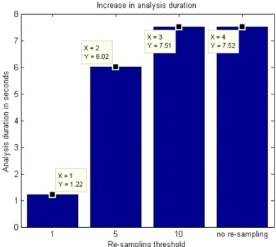
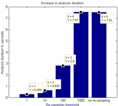
C8 D. Maxim, M. Houston, L. Santinelli, G. Bernat, R. Davis and L. Cucu-Grosjean, ”Re-Sampling for Statistical Timing Analysis of Real-Time Systems”, the 20th International Conference on Real-Time and Network Systems, ACM Digital Library, Pont `a Mousson, Novembre 2012
C7 D. Maxim, O. Buffet, L. Santinelli, L. Cucu-Grosjean and R. Davis, Op-timal Priority Assignment for Probabilistic Real-Time Systems, the 19th International Conference on Real-Time and Network Systems (RTNS), Nantes, September 2011
C6 L. Santinelli, P. Meumeu Yomsi, D. Maxim and L. Cucu-Grosjean, A Component-Based Framework for Modeling and Analyzing Probabilistic Real-Time Systems, the 16th IEEE International Conference on Emerg-ing Technologies and Factory Automation (ETFA), Toulouse, September 2011
We have studied the probabilistic response time analysis of systems with mul-tiple probabilistic parameters either by using bounds based on real-time cal-culus (J6, J4), extreme value theory (C9), direct calculation (J5, C11) or in
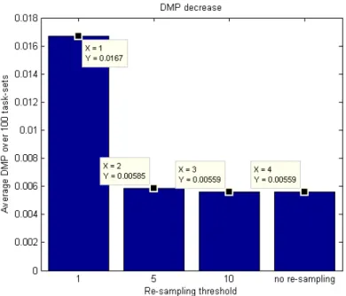
a context of component-based systems (C6). The probabilistic methods have, generally, high complexity and by upper-bounding the input probability dis-tributions we provide safe and faster results (C8). Worst-case reasoning is also provided to estimate statically the probabilistic worst-case execution time of a task (C10).
• Proposition of methods for obtaining probability distributions of the parame-ters of real-time systems. Obtaining these distributions is, generally, based on statistical methods. We have proposed and validated for the first time a statistical method for the estimation of probabilistic worst-case execution times of a program (task). This method is currently under patent submission and its details are confidential. Its exploitation plan concerns four different embedded industries (avionics, aerospace, automotive and rail) and related methods are also available:
J8 F. J. Cazorla, E. Quinones, T. Vardanega, L. Cucu-Grosjean, B. Triquet, G. Bernat, E. Berger, J. Abella, F. Wartel, M. Houston, L. Santinelli, L. Kosmidis, C. Lo and D. Maxim, ”PROARTIS: Probabilistically Analyz-able Real-Time System”, ACM Transactions on Embedded Computing Systems, 12(2s):94, 2013
J7 L. Yue, I. Bate, T. Nolte and L. Cucu-Grosjean, ”A New Way about using Statistical Analysis of Worst-Case Execution Times”, Special issue related to the WIP session of the 23rd Euromicro Conference on Real-Time Systems (ECRTS), ACM SIGBED Review, 8(3), September 2011 C13 F. Wartel, L. Kosmidis, C. Lo, B. Triquet, E. Quinones, J. Abella, A.
Gogonel, A. Baldovin, E. Mezzetti, L. Cucu, T. Vardanega and F. Ca-zorla, ”Measurement-Based Probabilistic Timing Analysis: Lessons from an Integrated-Modular Avionics Case Study”, the 8th IEEE International Symposium on Industrial Embedded Systems (SIES), Porto, June 2013 C12 L. Cucu-Grosjean, L. Santinelli, M. Houston, C. Lo, T. Vardanega, L.
Kosmidis, J. Abella, E. Mezzeti, E. Quinones and F. Cazorla, ”Measurement-Based Probabilistic Timing Analysis for Multi-path Programs”, the 24th Euromicro Conference on Real-Time Systems (ECRTS), Pissa, July 2012
We introduce the first static probabilistic timing analysis for randomized ar-chitectures in J8 and the corresponding measurement-based approach in C12. The hypotheses of the mathematical basis of a measurement-based method (as proposed in C12) may be fulfilled also by statistical treatment (J7). A case study of a measurement-based approach is provided for avionics in C13.
Organization of the chapter This chapter has three parts. The first part (Section 2.1) introduces the definitions and assumptions as well as the context of the results we present in Sections 2.3 and 2.2. In Section 2.2 we provide the response
time analysis published in C11. In Section 2.3 we provide the main details of the measurement-based probabilistic timing analysis published in C12. For both results we underline the differences between the independence between tasks and the independence as required by the probabilistic or the statistical method.
2.1
Definitions and assumptions. Context of the
prob-abilistic real-time systems
A random variableX1has associated a probability function (PF) f
X(.) with fX(x) =
P (X = x). The possible values X0, X1,· · · , XkofX belong to the interval [xmin, xmax],
where k is the number of possible values ofX . We associate the probabilities to the possible values of a random variable X by using the following notation
X = ✓ X0= Xmin X1 · · · Xk = Xmax fX(Xmin) fX(X1) · · · fX(Xmax) ◆ , (2.1) where Pki
j=0fX(Xj) = 1. A random variable may be also specified using its
cumu-lative distribution function (CDF) FX(x) =Pxz=xminfX(z).
Definition 8. The probabilistic execution time (pET) of the job of a task describes the probability that the execution time of the job is equal to a given value.
For instance the jth job of a task ⌧
i may have a pET
Cij = ✓ 2 3 5 6 105 0.7 0.2 0.05 0.04 0.01 ◆ (2.2) If fCj
i(2) = 0.7, then the execution time of the j
th job of ⌧
i has a probability of
0.7 to be equal to 2.
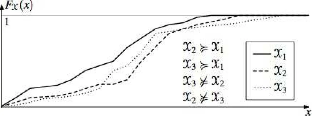
The definition of the probabilistic worst-case execution (pWCET) of a task is based on the relation ⌫ provided in Definition 9.
Definition 9. [49] Let X and Y be two random variables. We say that X is worse than Y if FX(x) FX(x), 8x, and denote it by X ⌫ Y.
For example, in Figure 2.1 FX1(x) never goes below FX2(x), meaning thatX2 ⌫
X1. Note that X2 and X3 are not comparable.
Definition 10. The probabilistic worst-case execution time (pWCET) Ci of a task
⌧i is an upper bound on the pETs Cij of all jobs of ⌧i 8j and it may be described by
the relation ⌫ as Ci⌫ Cij, 8j.
Graphically this means that the CDF of Ci stays under the CDF of Cij, 8j.
Following the same reasoning we define for a task ⌧i the probabilistic minimal
inter-arrival time (pMIT) denoted by Ti.