The turbulent dynamo as an instability in a noisy medium

HAL Id: hal-00001417

https://hal.archives-ouvertes.fr/hal-00001417v3

Submitted on 11 Dec 2006

HAL is a multi-disciplinary open access

archive for the deposit and dissemination of

sci-entific research documents, whether they are

pub-lished or not. The documents may come from

teaching and research institutions in France or

abroad, or from public or private research centers.

L’archive ouverte pluridisciplinaire HAL, est

destinée au dépôt et à la diffusion de documents

scientifiques de niveau recherche, publiés ou non,

émanant des établissements d’enseignement et de

recherche français ou étrangers, des laboratoires

publics ou privés.

The turbulent dynamo as an instability in a noisy

medium

Nicolas Leprovost, Bérengère Dubrulle

To cite this version:

Nicolas Leprovost, Bérengère Dubrulle. The turbulent dynamo as an instability in a noisy medium.

European Physical Journal B: Condensed Matter and Complex Systems, Springer-Verlag, 2005, 44,

pp.395. �10.1140/epjb/e2005-00138-y�. �hal-00001417v3�

hal-00001417, version 3 - 11 Dec 2006

(will be inserted by the editor)

The turbulent dynamo as an instability in a noisy medium

Groupe Instabilit´e et Turbulence,

CEA/DSM/DRECAM/SPEC and CNRS. URA 2464 F-91191 Gif sur Yvette Cedex, France e-mail: nicolas.leprovost@cea.fr

Received: date / Revised version: date

Abstract. We study an example of instability in presence of a multiplicative noise, namely the spontaneous generation of a magnetic field in a turbulent medium. This so-called turbulent dynamo problem remains challenging, experimentally and theoretically. In this field, the prevailing theory is the Mean-Field Dynamo [1] where the dynamo effect is monitored by the mean magnetic field (other possible choices would be the energy, flux,...). In recent years, it has been shown on stochastic oscillators that this type of approach could be misleading. In this paper, we develop a stochastic description of the turbulent dynamo effect which permits us to define unambiguously a threshold for the dynamo effect, namely by globally analyzing the probability density function of the magnetic field instead of a given moment.

PACS. 02.50.-r Probability theory, stochastic processes and statistics – 47.27.Gs Isotropic turbulence; homogeneous turbulence – 47.27.Jv High-Reynolds-number turbulence

Classical stability analysis are usually performed in systems were the control parameter is a non-fluctuating

quantity, e.g. for laminar flows in hydrodynamics. When the instability occurs in a random system (e.g. a

turbu-lent medium), resulting fluctuation of the control

param-eter, or multiplicative noise, may generate several surpris-ing effects that have been studied in a variety of systems.

The possibility of stabilization by noise has first been

ev-idenced on a Duffing oscillator [2] , where the solution x(t) = 0 is stable for values of the control parameter above

the deterministic threshold. This stabilization is generic for weak intensities of the noise. For stronger intensity,

however, noise induced transition may also arise in this

system [3]. In the case of a parametric instability, it has been showed experimentally [4] that the instability is

2 N. Leprovost and B. Dubrulle: The turbulent dynamo as an instability in a noisy medium

oscillatory bursts (corresponding to a signal with a vanish-ing mean but a most probable value equal to zero) appear

first when the control parameter is increased and are then replaced by a state where the most probable value is no

more equal to zero. On the contrary, in the subcritical

case, there is coexistence between these two states. This illustrates a central difficulty of instability in presence of

multiplicative noise associated with an ambiguity regard-ing the threshold value, which depends on the definition

of the order parameter [5].

The observations and techniques developed in these simple systems may be used to shed new light on some

recent issues associated with the dynamo effect, the

pro-cess of magnetic field generation through the movement of an electrically conducting medium. In this case, the

in-stability results from a competition between amplification of a seed magnetic field via stretching and folding, and

magnetic field damping through diffusion. In a laminar

fluid, it is controlled by a dimensionless number, the mag-netic Reynolds number (Rm), which must exceed some

critical value Rmc for the instability to operate. In a

tur-bulent medium, velocity fluctuations induce fluctuation

of the control parameter, making the turbulent dynamo problem similar to an instability in the presence of

multi-plicative noise. In that respect, recent numerical findings

such as observed in [6] may find a natural explanation. In their work, the authors observed short intermittent bursts

of magnetic activity separated by relatively long periods, increasing towards the bifurcation threshold. This feature

could be explained in terms of a supercritical instability in

presence of multiplicative noise since in this case, the bi-furcated state is generally composed of oscillatory bursts.

More generally, the multiplicative noise paradigm could turn useful to interprete the outcome of recent

experi-ments involving liquid metals. Among the various

operat-ing experiments, a clear distinction appears between set up with constrained or unconstrained geometry. In the

for-mer case [7], the fluctuation level is very weak. The veloc-ity field is then very close to its laminar (mean) value. In

these experiments, dynamos have been observed, at crit-ical magnetic Reynolds number comparable to the

theo-retical value. In contrast, unconstrained experiments [8]

are characterized by a large fluctuation level (as high as 50 per cent). A surrogate laminar Rmc can then be

com-puted, using the mean velocity field as an input [9] but it is not clear whether it will correspond to the actual dynamo

threshold, owing to the influence of turbulent fluctuations.

In this paper, we investigate this issue by techniques developed to study the Duffing oscillator and using a

stochas-tic description of small-scale turbulent motions. This sub-ject has been pioneered by Kazantsev [10], Parker [11]

and Kraichnan [12], and further developed by the Russian school [13]. It has recently been the subject of a renewed

interest, in the framework of anomalous scaling and

in-termittency [14], or computation of turbulent transport coefficients and probability density functions (PDF) [15].

The dynamic of the magnetic field B in an infinite

conducting medium of diffusivity η and velocity V, is gov-erned by the induction equation:

with control parameter built using typical velocity and scale as Rm = LV /η. We decompose the velocity field

into a mean part ¯Vi and a fluctuating part vi. In most

laboratory experiments, the mean part is provided by the

forcing. As such, it is generally composed of large scales,

while the fluctuating part collects all short time scale, small-scale movements. In this regard, it is natural to

con-sider the fluctuating part of the velocity as a noise, to be prescribed or computed in a physically plausible manner.

The simplest, most widely used shape is the Gaussian, delta-correlated fluctuations, the so-called “Kraichnan’s

ensemble”:

hvi(x, t)vj(x′, t′)i = 2Gij(x, x′)δ(t − t′) (2)

Equation (1) then takes the shape of a stochastic par-tial differenpar-tial equation for B. In that respect, we note

that the induction equation is linear and does not include explicit back reaction term allowing saturation of any

po-tential growth in the dynamo regime. This back reaction

is provided through the velocity which is subject to the Lorentz-Force, a quadratic form of B. It is usually ignored

in the so-called kinematic regime. However, for reasons which will become clearer later, we prefer to work with

a modified induction equation, so as to model this non-linear back reaction.

Indeed, the study of the induction equation alone could

be misleading when looking at the threshold of the dy-namo effect (it leads to a threshold value dependent on

the considered moment). This is symptomatic of the fact that the dynamo problem is nonlinear through the

Navier-Stokes equation. A practical way to include the effect of

the Lorentz force at the onset of the nonlinear regime is to add a saturating term in the induction equation.

Sym-metry considerations then favor a term like −cB2

Bi. In

some sense, this modification is akin to an amplitude

equa-tion, and the cubic shape for the non-linear term could be

viewed as the only one allowed by the symmetries. Such a procedure has been validated by [16] in the case of the

saturation of a Ponomarenko dynamo. Such a cubic form has also been evidenced by Boldyrev [15] by assuming the

equality of viscous and dynamical stresses in the Navier-Stokes equation at the onset of backreaction. In the sequel,

we show that the precise form of the nonlinear term does

not affect the threshold value, which only depends on the behaviour for |B| → 0. This is similar to the case of the

Duffing oscillator where the threshold is given by the Lya-punov exponent of the linearized oscillator [3].

A further difficulty is associated with the presence of

the diffusive terms. Their physical influence is to cut-out magnetic field Fourier components with wave numbers

ini-tially oriented in the contracting directions (stretching

di-rections for wave numbers). Through the divergence free condition, this favors magnetic field components

point-ing towards contractpoint-ing directions, thus counteractpoint-ing the initial effect of magnetic growth along stretching

direc-tion. The balance between these two effects yields the

dy-namo threshold ([18]). The direct consideration of diffu-sive terms in the stochastic formulation requires functional

derivative and integration, hindering simple analytical de-scription. We propose to model them partially through an

super-4 N. Leprovost and B. Dubrulle: The turbulent dynamo as an instability in a noisy medium

posed to and decorrelated from the velocity fluctuation [17], with correlation function < ξi(t)ξj(t′) >= 2ηδijδ(t −

t′_{). In the sequel, we show that this choice provides some}

sort of saturation for the moments of various order,

sim-ilar to the role of a viscosity. Damping of magnetic field

fluctuations, however, is not properly taken account by this model.

Using standard techniques [19,15], one can then derive

the evolution equation for P (B, x, t), the probability of

having the field B at point x and time t (we assume an homogeneous turbulence for simplicity):

∂tP = − ¯Vk∂kP − (∂kV¯i)∂Bi[BkP ] + ∂k[βkl∂lP ] (3)

+ c∂Bi[B

2

BiP ] + 2∂Bi[Bkαlik∂lP ]

+ µijkl∂Bi[Bj∂Bk(BlP )] ,

with the following turbulent tensors:

βkl = hvkvli + ηδkl, αijk= hvi∂kvji (4)

and µijkl= h∂jvi∂lvki .

The physical meaning of these tensors can be found by analogy with the “Mean-Field Dynamo theory”[1,20].

Indeed, consider the equation for the evolution of the mean

field, obtained by multiplication of equation (3) by Bi_and

integration:

∂thBii = − ¯Vk∂khBii + (∂kV¯i)hBki − 2αkil∂khBli

+ βkl∂k∂lhBii − chB 2

Bii. (5)

This equation resembles the classical Mean Field Equation of dynamo theory, with generalized (anisotropic) “α”and

“β”. The first effect leads to a large scale instability for

the mean-field, while the second one is akin to a turbulent diffusivity. A few remarks are in order at this point: i) our

mean field equation has been derived without assumption of scale separation. ii) The tensor µ does not appear at

this level. In the sequel, it will be shown to govern the

stochastic dynamo transition.

For this, we need to identify the threshold as a

func-tion of the noise properties. Here, we follow an idea by Mallick and Marcq [3], and focus on the properties of the

stationary PDF of the system. Indeed, below the transi-tion, the only stable state is B = 0 and the PDF should be

a Dirac delta function. Above the transition, other equi-librium states are possible, with non zero magnetic field.

However, in the general case, it is not possible to find analytical solution for the equation (3). We thus resort

to the following mean field argument. Changing variable

Bi= Bei where e is a unit vector (and can be

character-ized by d − 1 angular variables), we can get an equation

for P (B, ei, x) = JP (Bi) where J = Bd−1 is the

Jaco-bian of the transformation. We now assume that there is

an uncoupling for P as P (B, ei) = P (B)G(ei, x), and

per-form an average over the angular variables, to find a closed equation for P (B). In some sense, this can be regarded as

a kind of angle/action variable separation, with average over the fast variables. The final equation for P (B)

be-comes: ∂P ∂t = a ∂ ∂B[B ∂ ∂B(BP )] − b ∂ ∂B(BP ) + c ∂ ∂B(B 3 P ) (6)

where the coefficients are given by averages over the posi-tion and the angular variables h•iφ=R • G(e, x) dxde:

a = hµijkleiejekeliφ (7)

b = h∂kV¯ieiekiφ+ hµijkl(∆ikejel+ ∆kjeiel)iφ

where we used ∆ij = ∂ni(nj) = δij − eiej an

“angu-lar Dirac tensor”. One can notice that these coefficients only explicitly involve the tensor µ. Nevertheless, one must

keep in mind that the tensor α and β enter these

expres-sions by mean of the angular distribution G(ei, x), whose

expression involves this two tensors in the general case.

An obvious stationary solution of (6) is a Dirac func-tion, representing a solution with vanishing magnetic field.

Another stationary solution can be found by setting ∂tP =

0 in (6), with solution: P (B) = 1 ZB b/a−1_exph₋ c 2aB 2i (8)

where Z is a normalization constant. This solution can

represent a meaningful probability density function only if it can be normalized. This remark provides us with a

bifurcation threshold: there is dynamo whenever (8) is

in-tegrable, i.e., when solution other than vanishing magnetic field are possible.

Condition of integrability at infinity of (8) requires a be positive. This illustrates the importance of the

non-linear term which is essential to ensure vanishing of the probability density at infinity. Condition of integrability

near zero requires b/a be positive. This leads us to

iden-tify a necessary and sufficient condition for existence of a stationary dynamo as

a > 0 and b

a > 0 DY N AM O (9)

In some sense, this bifurcation (I) is obtained using the mean field as control parameter. Another bifurcation

thresh-old can be defined using the most probable field as control parameter. Indeed, an elementary calculation shows that

the condition for a maximum in the PDF is b > a.

There-fore, the bifurcation threshold (II) with the most probable field as control parameter is defined by b = a. This

differ-ence may have some relevance when analyzing real data from experiment. To illustrate this, we performed

simula-tions of the 1-D version of our non-linear stochastic sys-tem. It may be checked that the stationary PDF in this

case is exactly given by eq. (8). Therefore, the time series

and associated PDF are good illustration of the output of our 3D model, and the meaning of the two bifurcations

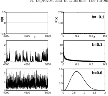
discussed above. The time series and PDF for three dif-ferent values of the control parameter are shown on figure

1.

The simulations show that the bifurcation (I) leads to an intermittent behavior for the magnetic field

reminis-cent of the characteristic behavior of instability in

pres-ence of multiplicative noise: typically, the magnetic energy exhibits bursts separated by long quiescent (zero magnetic

energy) period. Equation (8) cannot rigorously capture these intermittent states. However, two facts are very

sug-gestive of such a type of bifurcation in our solution: (a) the

distribution looks like a pure fluctuation distribution, with ill-defined mean value (b) the scaling for kBk ≪ 1

(mag-netic energy) is the same as that of [6]: P (kBk) = kBkγ

with γ = b/D − 1, where D is a “diffusion coefficient”for

6 N. Leprovost and B. Dubrulle: The turbulent dynamo as an instability in a noisy medium 4000 4500 5000 −0.5 0 0.5 t x(t) 0 0.1 0.2 0.3 0 100 200 x P(x) 40000 4500 5000 1 2 0 0.1 0.2 0.3 0 20 40 40000 4500 5000 1 2 0 0.5 1 1.5 2 0 0.5 1 1.5 b=−0.1 b=0.1 b=0.6

Fig. 1. Result of the surrogate 1D model: ∂tx= (b + ξ(t))x −

γx3

with hξ(t)ξ(t′_{)i = 2aδ(t − t}′_{). On the left side we show}

time series for a = 0.2, γ = 1 and 3 different values of the parameter b. On the right side, the corresponding PDF and the theoretical curve corresponding to equation (8).

bifurcation (II) is quite different in nature because of a well defined mean value for the magnetic field and

fluc-tuations around this mean. Note also that if we consider the dynamo instability in absence of noise, a = 0, the

two bifurcation threshold collapse. As stated by [6], the bifurcation corresponding to b > 0 may be difficult to

ob-serve in real experiments because, under the threshold,

the presence of the Earth external magnetic field always gives rise to magnetic fluctuations qualitatively similar to

that above the threshold (magnetic bursts separated by quiescent period). This effect can be taken into account

by adding an additive noise to equation (1).

In the theory of dynamical systems stability, the

insta-bility criterion is usually associated with the existence of a positive Lyapunov exponent for the growth of the system

energy: lim ln B2

/2t = lim ln B/t. It is possible to find

this exponent, by multiplying equation (6) by ln B and integrating with respect to B. This yields ∂thln Bi = b ,

meaning that the Lyapunov exponent in our system is equal to b. The two instability criteria (existence of a

nor-malizable solution or a positive Lyapunov exponent) are

therefore identical provided a > 0, a necessary condition for integrability of the PDF at infinity.

It is now interesting to discuss qualitatively the

mean-ing of our main result (9). It is possible to show that for isotropic or axisymmetric velocity fluctuations, the

coeffi-cient a is positive. So we suspect that the main condition for existence of a dynamo is positivity of b. Therefore, in

the limit of zero noise, the term proportional to µ is

negli-gible and the dynamo threshold is only determined by the condition h∂kV¯ieiekiφ > 0. Since the magnetic field will

mainly grow in the direction given by the largest eigen-value of Sij = ∂jV¯i and that the molecular diffusivity

will tend to orientate the magnetic field along contract-ing direction, the dynamo threshold will be the same as

in the deterministic case. Consider now a situation where

you increase the noise level. Two different influences on the sign of b then result: one through the factor

propor-tional by µ. According to the sign of this factor, it can therefore favor or hinder the dynamo. Another less

obvi-ous influence is through vector orientation. Indeed, noise

changes the distribution of magnetic field orientation. For example, if noise induces a flat distribution for ei, then

h∂kV¯ieiekiφ = Sii = 0. Even more dramatic results can

be obtained if the noise tends to align the vector along

case the factor h∂kV¯ieiekiφ becomes negative, decreasing

the dynamo threshold. From these two examples, one sees

that in the presence of noise, the dynamo threshold can be completely disconnected from the dynamo threshold

in the deterministic system ! Some caution is therefore in

order when designing an experiment based on mean field measurements.

Our approach gives a quantitative criterion on the

dy-namo threshold (namely b > 0). However, its practical

implementation requires the measure on the angular and position variables G(x, n, t) and the average of the tensor

µ with this measure. One can obtain the measure by in-tegrating equation (3) with respect to B. Unfortunately

the equation for G can not be solved in the general case and particular types of turbulence statistics have to be

considered (isotropic, axisymmetric, etc...). Work is under

progress to determine the angular measure in these simple cases. It is however interesting to note that this measure

explicitly involves the tensors α and β defined in (4) and appearing in the Mean Field Equations (5). In that sense,

the dynamo threshold depends on these tensors, albeit in a

less explicit way than in the Mean Field Equations (MFE). It would therefore be interesting to confront threshold

de-rived from (MFE), which are µ independent, and from our theory, to see what kind of error in the threshold

determi-nation one can expect by using MFE instead of the true,

non-perturbative theory.

AcknowledgmentsWe thank the Programme national de Plan´etologie, and the GDR Turbulence and GDR

Dy-namo for moral and financial support and F. Daviaud, K.

Mallick and P. Marcq for discussion and comments. We also thank Y. Pomeau for stimulating the study of the

intermittent dynamo and F. P´etr´elis for pointing out the link with the “on-off”intermittency.

References

1. F. Krause and K.-H. R¨adler, Mean field MHD and dynamo theory(Pergamon press, 1980).

2. R. Bourret, U. Frisch and A. Pouquet, Physica 65, 303 (1973); R. Graham and A. Schenzle, Phys. Rev. A 26, 1676 (1982); M. L¨ucke and F. Schank, Phys. Rev. Lett. 54, 1465 (1985).

3. K. Mallick and P. Marcq, Eur. Phys. J. B 36, 119 (2003); 38, 99 (2004).

4. S. Residori, R. Berthet, B. Roman and S. Fauve, Phys. Rev. Lett. 88, 024502 (2002); R. Berthet et al., Physica D 174, 84 (2003).

5. R. L. Stratonovich, Topics in the Theory of Random Noise (Gordon and Breach, 1967).

6. D. Sweet et al, Phys. Rev. E 63, 066211 (2001).

7. A. Gailitis et al., Phys. Rev. Lett. 84, 4365 (2000); R. Stieglitz and U. M¨uller, Phys. Fluids 13, 561 (2001). 8. N. L. Peffley, A. B. Cawthorne and D. P. Lathrop, Phys.

Rev. E 61, 5287 (2000); M. Bourgoin et al, Phys. Fluids 14, 3046 (2002).

9. L. Mari´e et al., Eur. Phys. J. B 33, 469 (2003); F. Ravelet, A. Chiffaudel, F. Daviaud and J. L´eorat, submitted to Phys. Fluids.

10. A. P. Kazantsev, Sov. Phys. JETP 26, 1031 (1968). 11. E. N. Parker, Astrophys. J. 162, 665 (1970).

8 N. Leprovost and B. Dubrulle: The turbulent dynamo as an instability in a noisy medium 12. R. H. Kraichnan and S. Nagarajan, Phys. Fluids 10, 859

(1967).

13. Ya. B. Zel’dovich, A. A. Ruzmaikin, S. A. Molchanov and D. D. Sokolov, J. Fluid Mech. 144, 1 (1984).

14. G. Falkovich, K. Gawedzki and M. Vergassola, Rev. Mod. Phys. 73, 913 (2001).

15. S. Boldyrev, Astrophys. J. 562, 1081 (2001).

16. F. P´etr´elis, PhD Thesis Paris VI, (2002); S. Fauve and F. Petrelis, The dynamo effect, in Peyresq Lectures on nonlinear phenomena (World scientific, 2003).

17. S. Pavel, S. Berloff and J. C. McWilliams, J. Phys. Oceanogr. 32, 797 (2002).

18. M. Chertkov, G. Falkovich, I. Kolokolov and M. Vergas-sola, Phys. Rev. Lett. 83, 4065 (1999).

19. J. Zinn-Justin, Quantum Field Theory and Critical Phe-nomena(Oxford, 2002).

20. H.K. Moffatt, Magnetic field generation in electrically con-ducting fluids(Cambridge University Press, 1978).