• Aucun résultat trouvé

A new criterion for the evaluation of the velocity field for rainfall-runoff modelling using a shallow-water model

N/A
N/A
Protected

Academic year: 2021

Partager "A new criterion for the evaluation of the velocity field for rainfall-runoff modelling using a shallow-water model"

Copied!
21
0
0

Texte intégral

(1)

HAL Id: hal-02956355

https://hal.archives-ouvertes.fr/hal-02956355

Submitted on 5 Oct 2020

HAL is a multi-disciplinary open access

archive for the deposit and dissemination of

sci-entific research documents, whether they are

pub-lished or not. The documents may come from

teaching and research institutions in France or

abroad, or from public or private research centers.

L’archive ouverte pluridisciplinaire HAL, est

destinée au dépôt et à la diffusion de documents

scientifiques de niveau recherche, publiés ou non,

émanant des établissements d’enseignement et de

recherche français ou étrangers, des laboratoires

publics ou privés.

A new criterion for the evaluation of the velocity field

for rainfall-runoff modelling using a shallow-water model

Florent Taccone, Germain Antoine, Olivier Delestre, Nicole Goutal

To cite this version:

Florent Taccone, Germain Antoine, Olivier Delestre, Nicole Goutal. A new criterion for the evaluation

of the velocity field for rainfall-runoff modelling using a shallow-water model. Advances in Water

Resources, Elsevier, 2020, 140, pp.103581. �10.1016/j.advwatres.2020.103581�. �hal-02956355�

(2)

A new criterion for the evaluation of the velocity field for

rainfall-runoff modelling using a shallow-water model

Florent Taccone

, Germain Antoine

, Olivier Delestre

, Nicole Goutal

§

October 5, 2020

Abstract

The aim of this work is to evaluate the accuracy of physically based models using the 2D Shallow Water Equations (SWE) for the simulation of rain-induced runoff. A key expectation of these models is to be able to reproduce properly both hydrograph at the outlet of the watershed and the associated velocity field within the spatial domain for a given rain event. However, this ability can be very challenging in mountainous environments, which include heterogeneous and high values of bottom slope and transient rain inputs. In this paper, we focused on both the error due to the numerical resolution of the SWE for low water depths runoff on steep slopes and that due to the physical representation of friction on the bottom for various water depth to roughness height ratios. Four test cases have been used, at different scales, to evaluate the model in comparison with experimental data. The first test case (from [Kirstetter et al., 2015]) was a rain induced flow in a straight channel. It allows to evaluate the error made for the chosen numerical resolution of the SWE and its impact on the velocity distribution in the domain (metric scale). A criterion defining an acceptable numerical error has been proposed. A second test case (from [Cea et al., 2014]), has been chosen for being also metric scaled and in the right range of the numerical error criterion. It allowed to evaluate the ability of a new friction law (adapted from [Lawrence, 1997]) to represent the measured velocity field in several inundation regimes at the metric scale. The third test case was a 40 m2 real plot studied by [Tatard et al., 2008]. On this test case, measured velocities have been compared with the simulated ones. Thanks to an infiltration source term added to the mass conservation equation, hydrographs at the outlet of the plot have been well reproduced, as well as the main part (including the highest values) of the measured velocities. In particular, the velocities are well represented when the criterion given in the first test case is satisfied. Finally, the model is applied to a real watershed with an area of 1 km2 on which hydrographs at the outlet have been successfully reproduced for two extreme rainy events [Le Bouteiller et al., 2015]. It appeared that both physical and numerical error were low in the hydrographic network and that the local velocities are correctly reproduced there, unlike in the hillslopes where the velocities are not well reproduced even if the mass fluxes are correct.

1

Introduction

In mountain areas, civil and industrial safety issues require an assessment of the sediment exportations over some very productive watersheds. As a first step, the comprehension and prediction of the sediment dynamic require a model capable of reproducing hydraulic transfers at the catchment scale, and more particularly to be able to reproduce local velocity field in runoff modelling. Thanks to the increasing computer capacities and the availability of high resolution DEM (Digital Elevation Models), it is becoming more and more relevant to use physically based models. The Shallow Water Equations (SWE) [de Saint-Venant, 1871] are widely used to rep-resent the overland flow ([Zhang and Cundy, 1989], [Gottardi and Venutelli, 1993], [Nord and Esteves, 2005], [Burguete et al., 2008], [Delestre et al., 2014], [Cea et al., 2014]). To solve these equations, two main challenges must be fixed. The first one concerns the numerical aspect of the problem, in particular the treatment of the wet/dry transitions with the presence of steep slopes over a large domain. The need to define a crite-rion to characterize the accuracy of the numerical resolution is then highlighted. The second challenge is the modelling of an essential physical process: the friction. Regarding the first challenge, many authors have dealt with different aspects of the numerical solution of the 2D Shallow Water models for runoff applications. Since the nineties, the finite volume method ([Bouchut, 2004], [Toro, 2009], [V´azquez-Cend´on, 2015]) is mainly used to solve the 2D Shallow Water Equations. Thus, it appears that the key point of this numerical res-olution is to preserve the positivity of the water depths, to deal with dry zones in presence of steep slope,

Laboratoire National d’Hydraulique et Environnement, EDF R&D, 6 Quai Watier 78400 Chatou France & Laboratoire d’Hydraulique Saint-Venant, 6 Quai Watier 78400 Chatou France

Laboratoire National d’Hydraulique et Environnement, EDF R&D, 6 Quai Watier 78400 Chatou France & Laboratoire d’Hydraulique Saint-Venant, 6 Quai Watier 78400 Chatou France

Universit´e Cˆote d’Azur, CNRS UMR 7351, LJAD, Parc Valrose, F-06108 Nice cedex 2, France & Engineering school Polytech Nice-Sophia

§Laboratoire National d’Hydraulique et Environnement, EDF R&D, 6 Quai Watier 78400 Chatou France & Laboratoire d’Hydraulique Saint-Venant, 6 Quai Watier 78400 Chatou France

(3)

and to be well-balanced in the sense of [Greenberg and LeRoux, 1996], meaning preserving the hydrostatic bal-ance of the lake at rest. In the literature, some numerical schemes have been developed to verify all these properties ([Kurganov and Petrova, 2007], [Gallardo et al., 2007], [Canestrelli et al., 2009], [Hou et al., 2014], [Cea and Blad´e, 2015], [Chertock et al., 2015], [Xia et al., 2017]). For the purpose of having a robust resolu-tion of the Shallow Water Equaresolu-tions for runoff applicaresolu-tions, the best compromise needs to be found between accuracy of the numerical scheme and the good properties above-mentioned. One common numerical method to respect states of equilibrium from a classical numerical scheme such as the HLLC scheme introduced by [Toro et al., 1994] or the kinetic scheme is the hydrostatic reconstruction introduced in [Audusse et al., 2004]. Nevertheless, in case of steep slopes and low water depths, the hydrostatic reconstruction needs very fine mesh (see [Delestre et al., 2012]) and this is not compatible with large scale applications like in entire wa-tershed. Several authors propose improvements of the hydrostatic reconstruction ([Caleffi and Valiani, 2009], [Bouchut and De Luna, 2010], [D´ıaz et al., 2013], [Morales de Luna et al., 2013], [Hou et al., 2014], [Xia et al., 2017]). In this paper, a modification of the hydrostatic reconstruction proposed by [Chen and Noelle, 2017] will be com-pared to experimental data at different scales from representative test cases of runoff applications and a criterion to qualify the numerical results will be defined. The second challenge concerns the modelling of the friction terms which is one of the essential physical processes for runoff applications. Indeed, in the presence of steep slopes, the solution of the Saint-Venant equations is provided by a slope-friction balance. Some limitations are encountered for the physical representation of important phenomena such as the effect of bottom friction on flow. The diversity of flows from rain-induced runoff leads to varied inundation regimes and the laws of friction are often specific to each regime. To represent the friction of water on the bottom, the model of [Lawrence, 1997] is chosen for its ability to represent different flow regimes. However, since this model is defined for turbulent flows, a Poiseuille friction law is used as in [Kirstetter et al., 2015] for laminar flows.

The key point of this study is to evaluate the relevance of a numerical model to represent the velocity field in a watershed with rain-induced runoff, using a friction law adapted to each turbulence and inundation regime. More generally, under which conditions the velocity field can be well represented and how much confidence one can have in numerical model for the velocity field representation.

The objectives of this paper are:

• to consider the different aspects of the problem: the numerical treatment of the slope source term and the physical representation of the friction term for application on a wide range of scales;

• to propose a double criterion to qualify the simulation results, and more particularly the relevance of the velocities. This double criterion is defined from both the theoretical error on the discretization of the source term [Chen and Noelle, 2017] and a heuristic analysis of the root mean square error on the laboratory test cases. The first criterion ensures the mesh convergence of the numerical scheme. The second criterion shows that in the case of low water depths and large slope gradients, it is possible to have well represented velocities in the model;

• to validate and deepen the whole methodology with representative test cases of increasing difficulty from laboratory experiments to real applications.

In this work, the model is confronted with velocity measurements at different scales and the velocity field is evaluated on a watershed application. Many works are interested in the representation of the velocity fields on a specific case ([Tatard et al., 2008], [Cea et al., 2014], [Kirstetter et al., 2015]) and some works that have addressed numerical problems on steep slopes at different scales with a focus on discharges at the domain outlet [Kim et al., 2012]. The key contribution of this work is to propose a method for evaluating velocities in the computational domain:

• at different scales, ranging from a laboratory channel of a few meters to a mountain watershed; • with steep slopes and friction laws adapted to each case;

• with a recent, simple and massively parallel numerical method.

The paper will be organized as follows: in the first section, the governing equations and the finite vol-ume scheme will be described and we will focus on the improvement of the hydrostatic reconstruction by the Chen and Noelle’s scheme. The theoretical error due to the discretization of the slope source term, given by [Chen and Noelle, 2017], is following a dimensionless number depending on the slope, the mesh size and the wa-ter depth. The friction modelling will be adressed in details. The second section will be dedicated to laboratory test cases used on one hand for the definition and validation of a heuristic criterion to qualify the simulation results and, on the other hand, the validation of the friction modelling. The first experiment is a laboratory case [Kirstetter et al., 2015] which simulates a rain induced runoff in a straight channel with a constant slope. It will be used to evaluate the error made on the numerical resolution of the Shallow Water Equations and its effects on the velocities. The second experiment is also a laboratory case, but with a more complex geometry [Cea et al., 2014]. It is a sinusoidal mould with a rough fixed bottom on which several types of flow are de-veloping. This allows the observation of the velocities for different inundation regimes and consequently the evaluation of the effect of the friction law. Finally, we present the results of the methodology on a more complex

(4)

test case. Data from an instrumented plot of 40 m2 in Thies (Senegal) have been selected [Tatard et al., 2008].

They are used to qualify velocities on a real field with rain induced runoff on a larger scale than laboratory experiments. The data of the Draix-Blone observatory in France [Le Bouteiller et al., 2015] are used for an application on the Laval watershed, a well instrumented watershed of about 1 km2. Even if the velocities are

not measured on this basin, their impact on the outlet discharge and catchment response will be evaluated.

2

Material and method

2.1

Overland flow simulation

The 2D Shallow Water Equations are derived from the Navier-Stokes equations with hydrostatic pressure and uniform vertical velocity assumptions [Gerbeau and Perthame, 2001]. These assumptions are available if the flow is shallow and the variations of the slope are not large [Gerbeau and Perthame, 2001]. They write:

             ∂h ∂t + ∂hu ∂x + ∂hv ∂y = R − I ∂hu ∂t + ∂hu2+gh22  ∂x + ∂huv ∂y = gh − ∂z ∂x− Sf x  ∂hv ∂t + ∂huv ∂x + ∂  hv2+ gh2 2   ∂y = gh  −∂z ∂y− Sf y  , (1)

where h is the water height, t the time, u the flow velocity in the x direction, v the flow velocity in the y direction, R the rain intensity, I the infiltration rate given by an infiltration model (see section 2.1.3), g the gravity constant, z the bottom elevation and Sf xand Sf ythe friction slope respectively in the x and y directions.

2.1.1 Numerical resolution

An unstructured mesh is used to discretize the domain in space. This allows better adaptation to the complex topography of a basin by better representing its topography and especially the shape of rivers and gullies in the river system. Using the formalism presented in [Audusse and Bristeau, 2005], a control volume is constructed at each node of the mesh, creating a boundary between each neighbor node of the mesh, as shown in figure1.

Figure 1: Representation of the formalism used for the 2D unstructured mesh resolution. The Shallow Water Equations (1) can be solved with a finite volume scheme which writes:

Uit+1= Uit−X j∈Vi  ∆t ∆xij Fijt + ∆t ∆xij Sijt  , (2)

where Uit = (hti, htiuti, htivti) the states at time t in the node Pi, Vi all the nodes surrounding Pi, ∆t the time

step, ∆xij= LCi

ij the space step with Ci the area of the cell constructed around the node Piand Lij the length

of the boundary edge between the cells Ci and Cj, Fijt is the numerical flux at the interface between the cells Ci

and Cj along nij, the normal vector to the boundary edge and Sijt = (Ri− Ii, stijx, stijy) are the source terms of

(5)

deal with the slope source terms st

ijxand stijy to respect the positivity of the water depth and the hydrostatic

balance and more particularly in case of wet/dry transitions and steep slopes applications.

The Shallow Water Equations are solved with the scheme (2) and the interface fluxes are calculated with the HLLC method [Toro et al., 1994]. The intermediate states involved in the flux calculation are defined as Uij = (hij, hijui, hijvi). The modified hydrostatic reconstruction method finally gives:

zij= min(max(zi, zj), min(hi+ zi, hj+ zj)),

hij = min(hi+ zi− zij, hi),

Sij= g2(hi+ hij)(zi− zij)nijLij.

Based on the definition given by [Chen and Noelle, 2017], a fully wet state when the water depth is higher than the bottom difference between two cells, and a partially wet regime otherwise, are distinguished at the interface of two cells (Figure2 illustrates these regimes).

Partially wet Fully wet

Figure 2: Illustration of the partially wet and fully wet regimes at the interface of two cells. If we consider the non dimensional number β = ∆x∂h

xz, if β is inferior to 1 the regime is partially wet and fully

wet otherwise. The exact error made on the source term then can be estimated. Indeed, [Chen and Noelle, 2017] give the theoretical slope source term error like:

Sij

Sex

= 1 − 1

2β, (3)

for the fully wet regime (β ≥ 1) and

Sij

Sex

= 1 − β

2, (4)

for the partially wet case (β < 1).

The simulations are performed in two dimensions with the open source computational code TELEMAC2D [Hervouet, 1999] mainly used in river applications. The computation code is parallelized with the MPI method. The computation times given in the next sections correspond to simulations on 56 cpu cores on Intel Xeon CPUs E5-2697 v3 - 2.60GHz. The presented scheme has been added the TELEMAC2D computation code and is available since the V8P0 version.

2.1.2 Friction term

Whatever the formulation considered, the friction term is computed with a semi-implicit treatment [Kirstetter et al., 2015]. [Bristeau and Coussin, 2001] demonstrated that the friction term Sf defined as:

Sf =

3νu

gh2, (5)

where ν is the water kinematic viscosity, is the approach that fits best with the data for the flume test case (section2.2.1). More generally, this formula is used to represent friction in cases where the flow is laminar.

For turbulent flows, the friction term defined by [Lawrence, 1997] is introduced to spatialize the friction term according to a constant size of roughness ks. This roughness size is linked to the Darcy-Weisbach coefficient

(6)

f =                       1 1.64 + 0.803ln(Λ) 2 if Λ ≥ 10 10 Λ2 if 1 ≤ Λ ≤ 10 8 πCDmin π 4, Λ  else , (6) with Λ = kh

s the inundation rate and CD the drag force of the rough particles fixed to 1 in [Lawrence, 1997].

With this formulation, the friction coefficient varies continuously for different inundation ratios and is related with the friction slope with the relation:

Sf =

f 8g

u|u|

h . (7)

It has been demonstrated in [Lawrence, 1997] that this friction model can fail for Reynolds numbers below 1000 and inundation ratios above 10 (Λ ≥ 10 in the equation (6)). In these cases, as the Reynolds number is low, the flow is laminar. By replacing the Lawrence’s friction model by the Poiseuille model, presented in the equation (5), a mixed friction model is introduced.

All these friction models are not yet available in the official version of TELEMAC2D and have been imple-mented for this work.

2.1.3 Infiltration model

An improvement of the [Green and Ampt, 1911] model, presented in [Brakensiek and Rawls, 1983] and [Esteves et al., 2000] is used to represent the infiltration in the model. It is a vertical 1D model computed at each cell of the domain.

As this infiltration model is only 1D vertical, its resolution is much faster than a 3D model with groundwater exchange like [Richards, 1931] type models. Moreover, the conductivity of the layers can be variable in the domain. The Horton model [Horton, 1933] is also widely used, but it does not allow to represent the vertical structure of the soil like this model. The infiltration rate is described like:

I = K  1 +hf+ h zf  , (8)

with K the soil conductivity under less than 1 cm of hydraulic head, hf the capillarity head and zf the wetting

front. Then, the wetting front is updated following the equation: zf =

IC

θs− θi

, (9)

with IC the cumulated height infiltrated since the beginning of the event, θs the saturated soil moisture or

the porosity and θi the initial soil moisture. In the watershed application, the soil is vertically divided in two

layers, a first one with an associated depth Zc and conductivity Kc and a second one with a depth considered

as infinite and a conductivity Ks. The conductivity K varies with the wetting front evolution according to this

equation:    K = Kc if zf ≤ Zc K = z zf f−Zc Ks + Zc Kc if zf > Zc . (10)

This model can be used with one or two layers depending on the nature of the soil in each case. Considering the thickness of the first layer as infinite allows to reduce it to a single-layer model. This single-layer model is used in particular in the case of the Thies instrumented plot. The use of the two-layer model is justified by the fact that the measurements carried out in the Laval watershed clearly show a different structure between the surface layer and the inner layer of the soil. Indeed, [Mathys, 2006] shows that for out of more than 160 profiles measured in the basin, there is a superficial structure, unstructured and porous of 8 cm deep on average. Deeper, there is a much more structured layer with less porosity. This model is not present in the TELEMAC2D official sources and has been added by the authors via users routine.

2.2

Experimental test cases

Four test cases are selected at different scales and degrees of complexity. First two laboratory test cases are selected with a simple geometry. The first laboratory case is used to evaluate the effect of the resolution method and the other one to evaluate the impact of the law of friction on local velocities. Then, the model is applied to a real case on a small plot to confirm the results of the two previous test cases. Finally, the model is evaluated over a watershed of about 1 km2 on which it is possible to reproduce the discharge at the outlet.

(7)

2.2.1 Flume experiment

[Kirstetter et al., 2015] provide data for a test case which is a straight channel of dimensions 4.04 m by 0.115 m. With a rain simulator over the domain, a steady rain, with an intensity of 25 mm/h or 50 mm/h depending on the chosen scenario, is applied during 600 s. The temporal evolution of the discharge at the outlet of this channel is observed with a time step of 0.1 s. This temporal evolution of the discharge is obtained by weighting the water flowing out of the channel. The water depth and the velocities are also measured along the channel every 60 cm when the steady state is reached. They are measured with a salt-tracing method [Planchon et al., 2005]. The dataset is available for three slope values: 2%, 5% and 25%. All slope and rain intensity configurations are used with the exception of the case with a slope of 5% and a rain intensity of 50 mm/h as no data are available on this case. The table1 summarizes the simulated cases. The infiltration is not taken into account.

Slope (%) Rain intensity (mm/h) Data available

2 25 X 5 25 X 25 25 X 2 50 X 5 50 25 50 X

Table 1: Configurations for the flume test case simulations.

2.2.2 Sinusoidal mould experiment

The second test case is a laboratory test case representing a real field with several values of inundation ratio [Cea et al., 2014]. At the inlet, runoff with water depths from 1 to 3 mm is observed, with high velocities. Then the flow is directed to furrows where the water depths can reach 2 cm. This test case is representative of the hydraulic transition which can be observed on a real plot with hydraulic jump between the runoff and the flow in the furrows. The number of furrows varies from one to three depending on the choice of the slope and the inlet discharge. Three configurations are considered. The basic configuration has an inflow of 94.12 cm3/s, a

mean slope of 11.54 %, so we have only the first furrow filled with water. In the second configuration, the mean slope is increased to 20.4 %, the inlet discharge stays close to the initial configuration 108.52 cm3/s and water is

flowing in the three furrows. The last configuration takes the same slope as the first configuration 11.54 %, but the inflow is three times higher: 291.15 cm3/s, and two furrows are supplied by water. The data available on this test case are measured at the steady state so they do not evolve in time. The water depths and the bottom elevation are measured with a laser scanner as presented in [Legout et al., 2012] in the whole domain with a spatial resolution of 0.5 mm and the experimental uncertainty of the water depth is 1 mm. Concerning the velocities, they are measured with the LSPIV method [Legout et al., 2012], with a spatial resolution of 5 mm and an experimental uncertainty of 0.1 m/s. Figure 3 shows the bottom topography of the sinusoidal mould. There is no infiltration in this test case.

(8)

2.2.3 Plot experiment

The third experiment is described in [Tatard et al., 2008]. The measurement site is located in Thies, Senegal. The plot is 10 m long and 4 m wide. An uniform rain is applied to the domain using a rain simulator as described in [Esteves et al., 2000]. After several rain events that have eroded the soil, the sediment mobility of the soil was considered as negligible and the soil is considered fixed for the period of interest. The soil is mainly composed of sand with a roughness size that will be considered spatially uniform. The average rain intensity applied by the simulator is 67 mm/h for 2 h. We note that there is a significant infiltration process in the domain because the total mass of rainfall does not correspond to the mass that was collected at the outlet. Velocities measurements were taken at 62 different locations on the plot. The measurement procedure is salt-tracing as in the first experimental case. Unlike the previous test case, there is no water level measurement in this case. Figure4shows the bottom topography of the plot and the location of the 62 velocity measurements. Some irregularities can be observed on the bottom topography which can mainly be due to measurement errors. However, since the true elevation of the bottom at these locations is not known, and they are quite far from each measurement point, the topography is kept as it is for the simulations. Overland flow models have already been tested on this dataset [Mugler et al., 2011].

Figure 4: Bottom elevation and velocity measurement points of the plot experiment in Thies.

2.2.4 Watershed application

The model is then evaluated by comparing results of the model to measured outlet discharges from field mea-surements on a real catchment. The Laval watershed is a sub-catchment of the Bouinenc watershed, located on the Draix-Bleone site [Le Bouteiller et al., 2015] in the Southern French Alps. The climate is a mountainous climate influenced by the Mediterranean climate which is reflected in particular by heavy summer storms and an average annual rainfall of 900 mm. Its total area is 0.86 km2and the mean slope is 58 %. The soil is mostly

constituted of black marls and 68% of the surface is a bare soil. At the outlet of the catchment, the data are available for many rainfall events with a time step of 60 s. The rainfall for every event is also measured every 60 s. The flow rate is evaluated by laser measurement of the water depth over a known fixed section. The size of the basin and the steep slopes cause the hydrological response to be fast. Consequently, the short and intense storm events lead to the highest flow rates at the outlet [Mathys, 2006]. Two different events are selected, one spring rain following three rainy days with a high soil moisture initial condition, and a summer storm with a dry initial soil state. The choice of these events is motivated by the fact that the initial state of the soil is very different from one to the other, but also because they are the two events that had the greatest impact on sediment transport in a year. Figure 5 shows the bottom topography of the Laval watershed. Different studies have been performed in this observatory, mainly related to sediment transport ([Lukey et al., 2000], [Bechet et al., 2016]), but also to hydrological processes [Esteves et al., 2005].

(9)

Figure 5: Bottom elevation of the Laval watershed.

3

Results

3.1

Flume experiment

The domain has been discretized in three triangular meshes with a space step of respectively 10 cm, 1 cm and 1 mm. Thus, the outlet discharge considered is rescaled for a width of 0.115 m. On the 1 mm mesh, the number of elements is 1.3 million and the computation time is about 3 hours. The simulation duration is 1000 s, the first 600 s representing the rise of the hydrograph and the steady state and the last 400 s the emptying of the domain. To evaluate the error between the simulation and the measurements, the root mean square error is calculated on the outlet discharge. Then, it is normalized by the mean values of the measured outlet discharge at the steady states. The error is first evaluated on the outlet discharge, because it is the most accurate data available for this test case. Indeed, velocities are measured at only seven points along the channel with uncertainties regularly exceeding 10%.

In this test case, the slope source terms treatment is crucial in the momentum conservation equation because the water depths are low and the slopes are steep. In addition, the equations (3) and (4) show that the numerical accuracy of the slope source terms treatment is strongly dependent on the mesh size (via the definition of β). The evolution of the water depth is regular in this test case, so the mean value in the domain at the steady state is considered as the representative depth for the calculation of β. In figure6, the simulations error made on the outlet discharge is compared with the theoretical error made on the source term depending on the value of β.

For the fully wet regime (β > 1), the RMSE on the outlet discharge follows the theoretical source term error. This result implies that we have a convergence in mesh size because whatever the slope and the positive water height defined, a mesh size can always be adapted to be in the case where β is large enough to minimize the error. But due to CPU limitation β could be less than 1 so the partially wet regime must be studied. There is no clear relation between the simulation error and the theoretical source term error. It appears that an error is made on the homogeneous problem, coming from the reconstructed values used in the calculation of the numerical fluxes. Focusing on the points that are in the partially-wet regime, it shows that the six points corresponding to the smallest errors are the simulations with a 25% slope. In addition, the two simulations corresponding to the smallest errors are the simulations with a rain intensity of 50 mm/h, and the error is very close for two different mesh sizes. Starting from these observations, it seems that the error made in the partially-wet case is not strongly dependent on the mesh size. Moreover, it seems to decrease when the slope and the water depths increase. By plotting the simulation error and the value of the water depth multiplied by the slope, a clear relation is highlighted in figure7. This result suggests that for the partially wet case, the error is decreasing when the slope source term gh∂xz is increasing.

To illustrate the impact of the numerical resolution on the velocities behavior in the domain, three simulations in particular are selected. The first case is the case where the error is minimal, i.e. the fully-wet case for which β is maximal. This is the case with a 50 mm/h rain on a 2% slope with a mesh size of 1 mm. Figure8 shows the simulated discharge compared to the experimental data at the channel outlet, but also the velocities along the channel at the steady state. This result shows that for a fully-wet case with a large enough value of β, the numerical resolution is accurate and the simulations fit well with the experimental data. The second case

(10)

0 0.1 0.2 0.3 0.4 0.5 0.6 0.7 0.001 0.01 0.1 1 10 100 RMSE β

Theoretical source term error Slope 2% Rain 25 mm/h S 2% R 50 mm/h S 5% R 25 mm/h S 25% R 25 mm/h S 25% R 50 mm/h

Figure 6: Normalized Root Mean Square Error made in the simulations compared to the theoretical source term error. 0.1 0.2 0.3 0.4 0.5 0.6 0.7 10-6 10-5 10-4 RMSE h∂xz (m) Simulations error

Figure 7: Relation between the normalized RMSE in the partially wet case and h∂xz.

chosen is where the error is maximal. This corresponds to a rainfall of 25 mm/h on a slope of 2% with a mesh size of 10 cm. In this case, a loss of quantity of movement is observed and the outlet discharge is very underestimated, as shown on figure8. The values of the mass fluxes at the steady part of the hydrograph show that the numerical scheme is mass conservative. This corresponds to the sum of the Fij terms in the equation

(2) at the output boundary condition. The simulated discharge presented here is the product between the longitudinal component of the velocity and the water depth (hu in the shallow water equations (1)). Therefore, the difference between the measured discharge and the experimental signal is directly related to the treatment of the slope source term in the momentum conservation equation. This also has an effect on the velocities, which are largely underestimated. The third case chosen is the case where the error is minimal when β is less than 1, when the term h∂xz is maximal. This is the case with a 25% slope, a rainfall of 50 mm/h and a mesh size of 10

cm. A discharge lower than the experimental discharge is observed at the outlet of the channel. However, the discharge obtained is greater than the one obtained in the previous case. Indeed, to compensate for the loss of motion quantity, the model slightly overestimates the velocities, as seen in figure8.

To sum up, velocities in the domain are well calculated when β is large enough. The criterion chosen to consider the error acceptable (RMSE<25%) is β > 2 for the fully wet case. However, this is not always possible, especially for flows with low water depths on steep slopes to construct a mesh fine enough to always be in this case. When β is lower than 1, the velocities can be significantly underestimated. Nevertheless, this only happens when the slope source term gh∂xz is small, and the velocities are a bit overestimated if it is large. The

criteria chosen to consider the error acceptable (RMSE<25%) is gh∂xz > 2 · 10−4m2/s2, and it is independent

(11)

0 1 2 3 4 5 6 7 0 200 400 600 800 1000 Outlet discharge (cm 3/s) t (s) Simulated discharge Measurements Simulated mass fluxes

0 0.01 0.02 0.03 0.04 0.05 0.06 0 0.5 1 1.5 2 2.5 3 3.5 4 V elocity (m/s) x (m) Simulation Measurements

Case 1: rain 50 mm/h, slope 2%, mesh size 1 mm

0 0.5 1 1.5 2 2.5 3 3.5 0 200 400 600 800 1000 Outlet discharge (cm 3/s) t (s) Simulated discharge Measurements Simulated mass fluxes

0 0.005 0.01 0.015 0.02 0.025 0.03 0.035 0 0.5 1 1.5 2 2.5 3 3.5 4 V elocity (m/s) x (m) Simulation Measurements

Case 2: rain 25 mm/h, slope 2%, mesh size 10 cm

0 1 2 3 4 5 6 7 0 200 400 600 800 1000 Outlet discharge (cm 3/s) t (s) Simulated discharge Measurements Simulated mass fluxes

0 0.02 0.04 0.06 0.08 0.1 0.12 0 0.5 1 1.5 2 2.5 3 3.5 4 V elocity (m/s) x (m) Simulation Measurements

Case 3: rain 50 mm/h, slope 25%, mesh size 10 cm

Figure 8: Temporal evolution of the outlet discharge (left) and velocities along the channel at the steady state (right) for the three chosen test cases, simulations vs measurements.

3.2

Sinusoidal mould experiment

In the previous section, a double criterion has been defined on a simple test case to evaluate the runoff resolution error and its impact on velocities in the domain. By evaluating the velocities under these criteria, which are β > 2 or gh∂xz > 2.10−4m2/s2, this second test case allows to study several types of inundation regime. Thanks

to its sinusoidal geometry, there are furrows in which the flow develops and between these furrows there is runoff with small water depths. The model is calibrated with the water depths, because it is the most accurate and a finely spatialized data available in this experiment. This measurement at the steady state is used to calibrate the representative size of the roughness in the friction law.

To choose the parameter of the roughness size ks in the [Lawrence, 1997]’s friction model (6), several

simu-lations have been made on each configuration. As the uncertainty measurement on the water depth is low, we choose to minimize the RMSE on this parameter. The minimal value of the RMSE is reached for a roughness size between 0.25 mm and 0.27 mm depending on the configuration. The value of ks is then fixed to 0.26 mm.

This value is coherent as the soil is made of grains between 0.5 mm and 1 mm and the roughness visible in the topography plays a role in slowing the flow. Moreover, the mesh sizes and the topographic measurements are fine enough to represent a part of these grains.

Accordingly to the flume test case, we created three triangular meshes with different grid sizes. The mesh sizes chosen are 10 mm, 5 mm and 2 mm for each configuration. For the finest mesh configuration, the number of elements is 536 654 and the computational time for 1000 s of simulation is about 7 minutes. The water depth in the furrow is well represented by the simulations for each tested configuration, as it is shown in figure9. The location of the hydraulic jump and the flow in the furrows are in good agreement with the experiments. Indeed, the maximum water depths, as well as the location of the hydraulic jumps at the entrance of the furrows are

(12)

very well reproduced. However, the water level is a little overestimated in the farthest furrows, especially in the experiments with three furrows.

Experiment Simulation

Configuration 1

Configuration 2

Configuration 3

Figure 9: Water depth (m) on the domain, experimental measure (left) versus simulation results (right) for the three configurations.

As shown in [Cea et al., 2014], the velocities measurement method can give inaccurate results where the water depths are small. In this test case, the main interest is in the physical representation of friction, so a filter is applied to the velocities and only those for which the numerical resolution is good are considered. Consequently, only velocities measurement points for which β is greater than 2 are therefore taken into account. The table 2 shows that the RMSE is smaller with the finest mesh, but the degradation of the spatial discretization does not impact significantly the accuracy.

Configuration ∆x (mm) RMSE (m/s) 1 2 0.0658396 5 0.0718715 10 0.0781000 2 2 0.0584047 5 0.0626524 10 0.071708 3 2 0.0384667 5 0.0410869 10 0.0471743 Table 2: Mesh convergence analysis on the velocities.

(13)

As said previously, the velocity measurement points on the domain are chosen under the criteria given in3.1, which means β is greater than 2, the slope being too gentle to be in the case where β < 1 and gh∂xz > 2.10−4

m2/s2. It is therefore considered that the resolution error is negligible and that friction formula plays a major

role in the velocities description. Figure10shows that the smallest velocities are well represented in the model, but the highest velocities are underestimated with the [Lawrence, 1997]’s friction model. The trend of the curve shows that the modeled velocities are limited. Indeed, high velocities do not seem to exceed a threshold for each simulation. The second configuration is also presented in [Cea et al., 2014] and the results are very similar.

By studying the distribution of Reynolds numbers in the domain, it appears that a velocity limitation often occurs for relatively small Reynolds numbers. In addition, figure10shows that there is no more limitation for the highest velocities with the mixed friction model. The roughness coefficient ks of the Lawrence’s model has

been recalculated in function of the water depth by minizing the RMSE as before. The new value found is 0.3 mm. The highest velocities are better represented by the model, even some unexplained underestimations remain for the test cases 1 and 2.

0 0.1 0.2 0.3 0.4 0.5 0 0.05 0.1 0.15 0.2 0.25 0.3 0.35 0.4 0.45 0.5 Simulated velocities (m/s) Measured velocities (m/s) Lawrence friction Mixed friction 0 0.05 0.1 0.15 0.2 0.25 0.3 0.35 0.4 0.45 0 0.05 0.1 0.15 0.2 0.25 0.3 0.35 0.4 0.45 Simulated velocities (m/s) Measured velocities (m/s) Lawrence friction Mixed friction 0 0.1 0.2 0.3 0.4 0.5 0.6 0 0.1 0.2 0.3 0.4 0.5 0.6 Simulated velocities (m/s) Measured velocities (m/s) Lawrence friction Mixed friction

Figure 10: Measured velocities compared to simulated velocities, comparison between the Lawrence’s friction model and the mixed friction model for the sinusoidal mould test case.

The Lawrence’s friction model is more accurate to represent the smallest velocities in the domain, but it is necessary to use the mixed friction model to represent the highest values of the velocities. In the perspective of a coupling with a erosion and deposition sedimentary model, these velocities are the most important contributors.

3.3

Plot experiment

This experiment has been chosen to evaluate whether the conclusions drawn from the laboratory experiments could be exported to a real plot. It also acts as a transition between laboratory cases and a real watershed, especially with the introduction of the infiltration model described in2.1.3. From a given average rainfall, the infiltration model is calibrated to reproduce the flow at the outlet of the plot. Then the velocities of the model are compared to measured velocities at several points. The error induced by the resolution of the shallow water is first evaluated on the velocities measurement points according to the conclusions drawn on the flume test case. Then, the goal is to see if the same limitation as on the sinusoidal mould test case is observed and if it is corrected by the mixed friction model.

On the plot, the finest mesh created is a 25 mm mesh, which corresponds to the resolution of the topographic data. This mesh has 137 921 elements and the computational time for the 8000 s simulation is about 7 minutes. The rain applied on the plot is variable with a mean value of 66.73 mm/h. The rain intensity is measured with rain gauges and fluctuations are observed around the mean value. These fluctuations are reflected in the outlet discharge observations. However, the salt-tracing velocity measurement technique requires a steady state in the plot. These fluctuations therefore lead to average several velocity measures spread over time. For the simulations, the choice made is to apply a constant rain to compare measured velocities with steady state

(14)

simulated velocities. Thus, the infiltration model is calibrated to reproduce the total amount of water exiting the domain during the rain event. Figure11 shows the measured and simulated total rain applied to the plot and the induced discharges at the outlet. To obtain this discharge with the Green-Ampt infiltration model, only one layer of soil is considered. The parameters used are:

• the layer conductivity: K = 7 mm/h, • the effective porosity: θs− θi= 0.125.

The behavior of the hydrograph is well reproduced with this infiltration model. The raise of the hydrograph is very coherent with the observations. However, the hydrograph is drying up a little bit more rapidly than that observed, which can be explained by the fact that exfiltration is not represented by the model.

0 0.2 0.4 0.6 0.8 1 1.2 0 1000 2000 3000 4000 5000 6000 7000 8000

Rain / outlet discharge (l/s)

Time (s)

Measured rain Input rain Measured discharge Simulated discharge

Figure 11: Rain and outlet discharge of the event in the plot for Thies case.

The simulated velocities are compared with the 62 measurement points when the flow rate is stabilized (t=7000s). To set the representative size of the bottom roughness, ksin the friction model, the RMSE on the

velocities is minimized. Unlike the previous experiment where the friction was set on the water depths, here only the measured velocities are available in the dataset. The parameter ks minimizing the RMSE is 0.37 mm

for both Lawrence’s friction and mixed friction model. Figure12represents the simulated velocities compared to the measured velocities in the domain. For both friction models, the highest velocities are well represented and an underestimation is observed for a part of the lowest velocities. The difference between the two friction models is observed only on the two points corresponding to the highest velocities.

Based on the results of the flume test case, the velocity can be underestimated for low values of β. This underestimation is observed for cases where β is less than 2 and the slope source term is not dominant (gh∂xz <

2.10−4). In this experiment, the slope is not steep enough to be in the case where β < 1 and gh∂xz > 2.10−4 so

we can distinguish two cases: the case where β ≤ 2 and the velocity is underestimated because of the numerical scheme and the case where β > 2 and the velocity is well represented. These two cases are highlighted in figure 12and explain the part where low velocities are underestimated.

0 5 10 15 20 25 30 0 5 10 15 20 25 30 Measured velocity (cm/s) Simulated velocity (cm/s) β < 2 β > 2 x=y 0 5 10 15 20 25 30 0 5 10 15 20 25 30 Measured velocity (cm/s) Simulated velocity (cm/s) β < 2 β > 2 x=y

Figure 12: Measured velocity compared to simulated velocities, comparison between the Lawrence’s friction model (left) and the mixed friction model (right) depending on the value of β for Thies case.

(15)

A mesh convergence analysis has been performed on this test case and the results are displayed in the table 3. It shows that the RMSE decreases with the mesh size. In addition, the topography is less well represented and the slopes are not strong enough for the source term to become dominant.

∆x (mm) RMSE (m/s) RMSE (m/s) Lawrence’s model mixed model 25 0.031507 0.030972 50 0.078562 0.078575 100 0.089981 0.089981

Table 3: Mesh convergence analysis on the velocities for Thies case.

To conclude, this experiment confirms the relevance of the use of the simplified Green-Ampt infiltration model to estimate the outlet discharge. The velocity behavior corroborates the results obtained from the two laboratory experiments. Velocities are underestimated when β is less than 2 due to the limitations of the numerical scheme highlighted in the flume test case. The two highest velocities are underestimated if the Lawrence model is located in the well inundated case with Reynolds numbers below 1000, which is corrected by the mixed friction model as shown in the sinusoidal mould test case. However, the larger is the mesh size, the smaller is the difference between the models. The choice of the mixed friction model is thus relevant for small scale experiment, especially to represent the highest velocities, but its impact is limited when the scale and the mesh size is increased.

3.4

Watershed application

The model is now applied to a real watershed on which outlet discharge measurements are available. At this scale, the finest mesh size used is 1 m and the Lawrence’s friction model and the mixed friction model give the same results. The goal is to observe the effect of the numerical resolution on the representation of the outlet discharges.

On this domain, three mesh sizes are considered, with a space step of 1 m, 2 m and 5 m. The 1 m mesh has almost 2 millions elements and the computational time for a simulation is about 30 minutes. In the hydraulic network, the mesh is forced to follow the lowest point of the river. This leads to a greater representation of the channels geometry, in particular for the coarser mesh, and the water is flowing in the river direction. The model is calibrated to field data by comparing the measured and simulated outlet discharges on two events. The events are selected because they are the most erosive of the 2012 year, in terms of sediment volume exported at the outlet. The first event is recorded the 29th of May succeeding six rainy events from the 21st to the 27th of May. The maximal value of the rain intensity is 84 mm/h and the peak discharge is 3 m3/s. Concerning the

other event, it is a summer storm of the 25th August with an initial dry state, the last recorded event being the 25th July. The maximal intensity of the rain is 156 mm/h and the peak discharge is 6.6 m3/s.

To simulate these events, we set the properties of the soil constant in time and space, modifying only the initial soil moisture (θi in the infiltration model). The calibration has been performed on the finest mesh and

gives the following soil parameters: • first layer thickness: Zc = 80 mm,

• first layer porosity: θ1 = 0.35,

• first layer conductivity: Kc = 30 mm/h,

• second layer porosity: θ2 = 0.25,

• second layer conductivity: Ks = 1 mm/h,

• capillarity head: hf = 50 mm.

Inspired by the measurements of [Mathys, 2006], the parameters are chosen to have a porous surface layer and a more structured base layer. The value chosen for the base layer conductivity is clearly underestimated to balance the effects of the exfiltration, which is not represented by the model. the parameters representing the soil properties have been set to be as close as possible to the measurements. Then, the calibration process was carried out in two steps: a first step in which the initial water content was set to represent the peak intensity for each event, and a second step in which the representative size of the roughness was set according to the peak arrival time for the two events. The initial soil moisture is set to θi=0.22 for the spring event and θi=0.03 for

the summer storm. Figure13presents the measured and simulated outlet discharges for the spring event and the summer event. The simulated results are in good agreement with the observations. The outlet hydrographs are well represented for the two events, especially for the 1 m and 2 m meshes. For the 5 m mesh, the flow is slowed and a dephasing is observed. The table 4 shows the RMSE on the outlet hydrographs normalized by each maximal value for the two events.

(16)

Event ∆x (m) RMSE (-) 29/05/2012 1 0.041959 2 0.052898 5 0.239660 28/08/2012 1 0.025281 2 0.028930 5 0.155558

Table 4: RMSE on the outlet hydrographs for each event and each mesh size for the watershed case.

0 0.5 1 1.5 2 2.5 3 3.5 0 1000 2000 3000 4000 5000 0 20 40 60 80 100 Outlet discharge (m 3/s) Rain intensity (mm/h) Time (s) dx=1m dx=2m dx=5m Rain Measurement 0 1 2 3 4 5 6 7 0 1000 2000 3000 4000 5000 6000 7000 0 50 100 150 200 Outlet discharge (m 3/s) Rain intensity (mm/h) Time (s) dx=1m dx=2m dx=5m Rain Measurement

Figure 13: Measured outlet discharge compared to simulated results for the watershed case.

The mixed friction model is used with a roughness size fixed to 5 cm, as the RMSE on the outlet discharge is minimized for this roughness size. Figure14shows the RMSE in function of the roughness size parameter of the Lawrence’s friction model, and both events are minimized for the same value.

0.02 0.04 0.06 0.08 0.1 0.12 0.14 0.16 0.18 1 2 3 4 5 6 7 8 9 10

RMSE normalized on the outlet discharge

Roughness size (cm)

Summer event Spring event

Figure 14: Normalized RMSE on the outlet discharge for the two events considered for the watershed case. The soil properties are considered as uniform in space, as well as the friction coefficient. The representation of the vertical structure of the soil is sufficient to have a satisfactory reproduction of the hydrographs. By isolating the areas where the error on the resolution is low according to the criteria given in3.1, it appears that in the hydraulic network one has a good representation of the velocities by the numerical scheme. However, figure15shows that the dynamic is a little different for the two events. For the spring event where the soil is already wet and therefore the infiltration capacity is lower, the well resolved zone is better distributed upstream of the network. Concerning the summer event, the infiltration capacity is higher, but also is the discharge. The quantity of water concerned by the well resolved zone is more important downstream of the basin, but is less high in the network. The accuracy of the hydrographs seems to be in relation with the presence of large well resolved zones close to the outlet, where the discharge is measured. Indeed, the RMSE of the simulated outlet hydrograph of the summer event is much lower than the one for the spring event.

(17)

29th May, spring event

28 August, summer event

Hydraulic network and mesh representation

Figure 15: Location of areas with minimal resolution error for the watershed case.

4

Conclusion

This paper focuses on the relevance of the Shallow Water Equations to model rain-induced runoff modelling and particularly on the evaluation of the local velocities. Four experimental test cases were used to analyze and assess the numerical model and to better understand its behavior. The first experiment is a flume with a constant slope on which drops a constant rain used to evaluate the error due to the numerical scheme. The second test case is a sinusoidal mould with furrows representing the agricultural terrain. Then the conclusions from these two laboratory experiments were used to interpret the simulated results obtained on the Thies test case (10 meters long real sandy plot) in comparison with measurements. Finally, the model was applied on a real catchment (Laval catchment, in the southern French Alps) where only outlet discharge measurements were

(18)

available.

The flume test case demonstrates that the error of the numerical resolution with the [Chen and Noelle, 2017]’s scheme can be quantified. This test case shows explicitly that this numerical error can lead to very important deviations on the simulated velocities for well reproduced mass fluxes. Thus, two criteria were defined to repro-duce conditions in which the error is acceptable. The first one is verified if the water depth is two times higher than the bottom elevation difference between two adjacent cells. The second criterion is verified if the slope and the runoff water level are high enough for the slope source term gh∂xz to be greater than 2 · 104 m2/s2.

The [Lawrence, 1997]’s friction model was used for its ability to reproduce a wide range of inundation ratios. Comparisons with velocities of the second test case showed that Lawrence’s friction model is well adapted but presents a limitation to reproduce the highest velocities. This limitation was corrected by adding a laminar friction law to better represent the velocities in a well inundated regime combined with low Reynolds numbers. The difference between Lawrence’s model and the mixed friction model became less visible when the mesh size was larger, which was the case for larger scale applications (Thies plot and Laval watershed test cases).

On the Thies plot test case, the numerical error criterion allowed to discriminate well reproduced velocities from the other ones. When the numerical criteria are respected, the mixed friction model gave very good results compared to the measured velocities. The error coming from the friction representation could not be compared with the error coming from the numerical resolution, but the numerical criterion found was able to frame the good representation of the velocities.

On the Laval watershed, two rainy events with two different seasons and initial conditions were selected. The outlet hydrographs were well reproduced on both events with the mixed friction model. The numerical criterion showed that the velocities are well reproduced mainly in the hydraulic network. Depending on the initial soil moisture and the rain intensity, the well resolved zone (the zone respecting the numerical criterion) spread more or less in the gullies upstream.

This work proposes a new methodology to evaluate the quality of the representation of the velocity field in a watershed for rain-induced runoff. It highlights well known problems in solving the Shallow Water Equations in the presence of steep slopes and low water depths ([Delestre et al., 2012], [Kim et al., 2012]). This provides an objective criterion for evaluating the discretization of the slope source term in a real case. This was possible thanks to a friction law identification work adapted to each studied test case allowing to neglect the impact of the physical representation of this one compared to the numerical error committed on the discretization of the slope source term.

Moreover, this methodology is built using a first-order numerical scheme implemented in open source com-putational code. This, combined with the choice of the right friction law for each case, makes this methodology transferable to other numerical schemes, and can be used as a basis for an objective choice of the numerical method to be used for velocity modelling for rain-induced runoff cases.

Acknowledgements

This work is a part of EDF R&D thesis within the CIFRE agreement number 2015/1102. The authors would like to thank O. Planchon, G. Nord, C. Le Bouteiller and E. Audusse for the constructive discussions.

References

[Audusse et al., 2004] Audusse, E., Bouchut, F., Bristeau, M.-O., Klein, R., and Perthame, B. (2004). A fast stable well-balanced scheme with hydrostatic reconstruction for shallow water flows. SIAM Journal on Scientific Computing, 25(6):2050–2065,https://doi.org/10.1137/S1064827503431090.

[Audusse and Bristeau, 2005] Audusse, E. and Bristeau, M.-O. (2005). A well-balanced positivity ”second-order” scheme for shallow water flows on unstructured meshes. Journal of Computational Physics, 206:311– 333,https://doi.org/10.1016/j.jcp.2004.12.016.

[Bechet et al., 2016] Bechet, J., Duc, J., Loye, A., Jaboyedoff, M., Mathys, N., Malet, J.-P., Klotz, S., Le Bouteiller, C., Rudaz, B., and Travelletti, J. (2016). Detection of seasonal cycles of erosion processes in a black marl gully from a time series of high-resolution digital elevation models (DEMs). Earth Surf. Dynam., 4:781–798,https://doi.org/10.5194/esurf-4-781-2016.

[Bouchut, 2004] Bouchut, F. (2004). Nonlinear Stability of Finite Volume Methods for Hyperbolic Conservation Laws and Well-Balanced Schemes for Sources.

[Bouchut and De Luna, 2010] Bouchut, F. and De Luna, T. M. (2010). A subsonic-well-balanced reconstruction scheme for shallow water flows. SIAM Journal on Numerical Analysis, 48(5):1733–1758,https://doi.org/ 10.1137/090758416.

[Brakensiek and Rawls, 1983] Brakensiek, D. L. and Rawls, W. J. (1983). Agricultural management effects on soil water processes part II: Green and Ampt parameters for crusting soils. Transactions of the ASAE, 26(6):1753–1757,https://doi.org/10.13031/2013.33838.

(19)

[Bristeau and Coussin, 2001] Bristeau, M.-O. and Coussin, B. (2001). Boundary conditions for the shal-low water equations solved by kinetic schemes. Technical Report 4282, INRIA, https://hal.inria.fr/ inria-00072305.

[Burguete et al., 2008] Burguete, J., Garcia-Navarro, P., and Murillo, J. (2008). Friction term discretization and limitation to preserve stability and conservation in the 1d shallow-water model: Application to unsteady irrigation and river flow. International Journal for Numerical Methods in Fluids, 58:403–425,https://doi. org/10.1002/fld.1727.

[Caleffi and Valiani, 2009] Caleffi, V. and Valiani, A. (2009). Well-balanced bottom discontinuities treatment for high-order shallow water equations WENO scheme. Journal of Engineering Mechanics, 135:684–696, https://doi.org/10.1061/(ASCE)0733-9399(2009)135:7(684).

[Canestrelli et al., 2009] Canestrelli, A., Siviglia, A., Dumbser, M., and Toro, E. F. (2009). Well-balanced high-order centred schemes for non-conservative hyperbolic systems. applications to shallow water equations with fixed and mobile bed. Advances in Water Resources, 32(6):834–844, https://doi.org/10.1016/j. advwatres.2009.02.006.

[Cea and Blad´e, 2015] Cea, L. and Blad´e, E. (2015). A simple and efficient unstructured finite volume scheme for solving the shallow water equations in overland flow applications. Water resources research, 51(7):5464– 5486,https://doi.org/10.1002/2014WR016547.

[Cea et al., 2014] Cea, L., Legout, C., Darboux, F., Esteves, M., and Nord, G. (2014). Experimental validation of a 2D overland flow model using high resolution water depth and velocity data. Journal of Hydrology, 513:142–153,https://doi.org/10.1016/j.jhydrol.2014.03.052.

[Chen and Noelle, 2017] Chen, G. and Noelle, S. (2017). A new hydrostatic reconstruction scheme based on subcell reconstructions. SIAM Journal on Numerical Analysis, 55(2):758–784, https://doi.org/10.1137/ 15M1053074.

[Chertock et al., 2015] Chertock, A., Cui, S., Kurganov, A., and Wu, T. (2015). Well-balanced positivity preserving central-upwind scheme for the shallow water system with friction terms. Int. J. Numer. Meth. Fluids, 78:355–383,https://doi.org/10.1002/fld.4023.

[de Saint-Venant, 1871] de Saint-Venant, A. B. (1871). Th´eorie du mouvement non permanent des eaux, avec application aux crues des rivi`eres et `a l’introduction des mar´ees dans leur lit. Technical report, Acad´emie des Sciences.

[Delestre et al., 2014] Delestre, O., Cordier, S., Darboux, F., Du, M., James, F., Laguerre, C., Lucas, C., and Planchon, O. (2014). FullSWOF: A software for overland flow simulation. In Advances in hydroinformatics, pages 221–231. Springer,https://doi.org/10.1007/978-981-4451-42-0_19.

[Delestre et al., 2012] Delestre, O., Cordier, S., Darboux, F., and James, F. (2012). A limitation of the hydro-static reconstruction technique for shallow water equations. Comptes Rendus de l’Acad´emie des Sciences -Series I, 350:677–681,https://doi.org/10.1016/j.crma.2012.08.004.

[D´ıaz et al., 2013] D´ıaz, M. C., L´opez-Garc´ıa, J. A., and Par´es, C. (2013). High order exactly well-balanced numerical methods for shallow water systems. Journal of Computational Physics, 246:242–264, https:// doi.org/10.1016/j.jcp.2013.03.033.

[Esteves et al., 2005] Esteves, M., Descroix, L., Mathys, N., and Lapetite, J. M. (2005). Soil hydraulic properties in a marly gully catchment (Draix, France). Catena, 63:282–298, https://doi.org/10.1016/j.catena. 2005.06.006.

[Esteves et al., 2000] Esteves, M., Faucher, X., Galle, S., and Vauclin, M. (2000). Overland flow and infiltration modelling for small plots during unsteady rain: numerical results versus observed values. Journal of Hydrology, 228:265–282,https://doi.org/10.1016/S0022-1694(00)00155-4.

[Gallardo et al., 2007] Gallardo, J. M., Par´es, C., and M., C. (2007). On a well-balanced high-order finite volume scheme for shallow water equations with topography and dry areas. Journal of Computational Physics, 227:574–601,https://doi.org/10.1016/j.jcp.2007.08.007.

[Gerbeau and Perthame, 2001] Gerbeau, J. F. and Perthame, B. (2001). Derivation of viscous Saint Venant system for laminar shallow water; numerical validation. Discrete and Continuous Dynamical Systems, 1(1):89– 102,https://doi.org/10.3934/dcdsb.2001.1.89.

[Gottardi and Venutelli, 1993] Gottardi, G. and Venutelli, M. (1993). A control-volume finite-element model for two-dimensional overland flow. Advances in Water Resources, 16(5):277–284, https://doi.org/10.1016/ 0309-1708(93)90019-C.

(20)

[Green and Ampt, 1911] Green, W. H. and Ampt, G. A. (1911). Studies on soil physics. The Journal of Agricultural Science, 4:1–17,https://doi.org/10.1017/S0021859600001441.

[Greenberg and LeRoux, 1996] Greenberg, J. M. and LeRoux, A. Y. (1996). A well-balanced scheme for the numerical processing of source terms in hyperbolic equations. SIAM Journal on Numerical Analysis, 33(1):1– 16,https://doi.org/10.1137/0733001.

[Hervouet, 1999] Hervouet, J. M. (1999). TELEMAC, a hydroinformatic system. La houille blanche, 3:21–28, https://doi.org/10.1051/lhb/1999029.

[Horton, 1933] Horton, R. E. (1933). The role of infiltration in the hydrologic cycle. American Geophysical Union, pages 446–460,https://doi.org/10.1029/TR014i001p00446.

[Hou et al., 2014] Hou, J., Simons, F., Liang, Q., and Hinkelmann, R. (2014). An improved hydrostatic reconstruction method for shallow water model. Journal of Hydraulic Research, 52(3):432–439, https: //doi.org/10.1080/00221686.2013.858648.

[Kim et al., 2012] Kim, J., Warnock, A., Ivanov, V. Y., and Katopodes, N. D. (2012). Coupled modeling of hydrologic and hydrodynamic processes including overland channel flow. Advances in Water Resources, 37:104–126,https://doi.org/10.1016/j.advwatres.2011.11.009.

[Kirstetter et al., 2015] Kirstetter, G., Hu, J., Delestre, O., Darboux, F., Lagr´ee, P. Y., Popinet, S., Fullana, J. M., and Josserand, C. (2015). Modeling rain-driven overland flow: empirical versus analytical friction terms in the shallow water approximation. Journal of Hydrology, 536:1–9, https://doi.org/10.1016/j. jhydrol.2016.02.022.

[Kurganov and Petrova, 2007] Kurganov, A. and Petrova, G. (2007). A second-order well-balanced positivity preserving central-upwind scheme for the Saint-Venant system. Communications in Mathematical Sciences, 5:133–160,https://projecteuclid.org/download/pdf_1/euclid.cms/1175797625.

[Lawrence, 1997] Lawrence, D. S. L. (1997). Macroscale surface roughness and frictional resistance in overland flow. Earth Surface Processes and Landforms, 22:365–382.

[Le Bouteiller et al., 2015] Le Bouteiller, C., Klotz, S., Li´ebault, F., and Esteves, M. (2015). Observatoire hydros´edimentaire de montagne Draix-Bl´eone. IRSTEA.

[Legout et al., 2012] Legout, C., Darboux, F., N´ed´elec, Y., Hauet, A., Esteves, M., Renaux, B., Denis, H., and Cordier, S. (2012). High spatial resolution mapping of surface velocities and depths for shallow overland flow. Earth Surface Processes and Landforms, 37(9):984–993,https://doi.org/10.1002/esp.3220.

[Lukey et al., 2000] Lukey, B. T., Sheffield, J., Bathurst, J. C., Hiley, R. A., and Mathys, N. (2000). Test of the SHETRAN technology for modelling the impact of reforestation on badlands runoff and sediment yield at Draix, France. Journal of Hydrology, 235:44–62,https://doi.org/10.1016/S0022-1694(00)00260-2. [Mathys, 2006] Mathys, N. (2006). Analyse et mod´elisation `a diff´erentes ´echelles des m´ecanismes d’´erosion et

de transport de mat´eriaux solides. Cas des petits bassins versants de montagne sur marne (Draix, Alpes-de-Haute-Provence). PhD thesis, INP Grenoble,https://hal.inrae.fr/tel-02588905.

[Morales de Luna et al., 2013] Morales de Luna, T., Castro D´ıaz, M. J., and Par´es, C. (2013). Reliability of first order numerical schemes for solving shallow water system over abrupt topography. Applied Mathematics and Computation,https://doi.org/10.1016/j.amc.2013.03.033.

[Mugler et al., 2011] M¨ugler, C., Planchon, O., Patin, J., Weill, S., Silvera, N., Richard, P., and Mouche, E. (2011). Comparison of roughness models to simulate overland flow and tracer transport experiments under simulated rainfall at plot scale. Journal of Hydrology, 402:25–40, https://doi.org/10.1016/j.jhydrol. 2011.02.032.

[Nord and Esteves, 2005] Nord, G. and Esteves, M. (2005). PSEM2D: A physically based model of erosion processes at the plot scale. Water Resources Research, 41,https://doi.org/10.1029/2004WR003690. [Planchon et al., 2005] Planchon, O., Silvera, N., Gimenez, R., Favis-Mortlock, D., Wainwright, J., Le

Bisson-nais, Y., and Govers, G. (2005). An automated salt-tracing gauge for flow-velocity measurement. Earth Surface Processes and Landforms, 30:833–844,https://doi.org/10.1002/esp.1194.

[Richards, 1931] Richards, L. A. (1931). Capillary conduction of liquids through porous mediums. Physics, 1(5):318–333,https://doi.org/10.1063/1.1745010.

[Tatard et al., 2008] Tatard, L., Planchon, O., Wainwright, J., Nord, G., Favis-Mortlock, D., Silvera, N., Ribolzi, Esteves, M., and Huang, C. H. (2008). Measurement and modelling of high-resolution flow-velocity data under simulated rainfall on a low-slope sandy soil. Journal of Hydrology, 348:1–12, https: //doi.org/10.1016/j.jhydrol.2007.07.016.

(21)

[Toro, 2009] Toro, E. F. (2009). Riemann Solvers and Numerical Methods for Fluid Dynamics. Springer. [Toro et al., 1994] Toro, E. F., Spruce, M., and Speares, W. (1994). Restoration of the contact surface in the

HLL-Riemann solver. Shock Waves, 4:25–34,https://link.springer.com/article/10.1007/BF01414629. [V´azquez-Cend´on, 2015] V´azquez-Cend´on, E. (2015). Solving Hyperbolic Equations with Finite Volume Methods.

Springer.

[Xia et al., 2017] Xia, X., Liang, Q., Ming, X., and Hou, J. (2017). An efficient and stable hydrodynamic model with novel source term discretization schemes for overland flow and flood simulations. Water Resources Research, 53,https://doi.org/10.1002/2016WR020055.

[Zhang and Cundy, 1989] Zhang, W. and Cundy, T. W. (1989). Modeling of two-dimensional overland flow. Water Resources Research, 25(9):2019–2035,https://doi.org/10.1029/WR025i009p02019.

Figure

Figure 1: Representation of the formalism used for the 2D unstructured mesh resolution.
Figure 2: Illustration of the partially wet and fully wet regimes at the interface of two cells.
Figure 3: Bottom elevation of the sinusoidal mould experiment.
Figure 4: Bottom elevation and velocity measurement points of the plot experiment in Thies.
+7

Références

Documents relatifs

Due to the progressive compaction of volcanic materials with pressure, temperature and time (e.g. This suggests that the heterogeneity of these structures should also

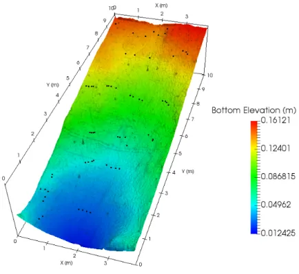
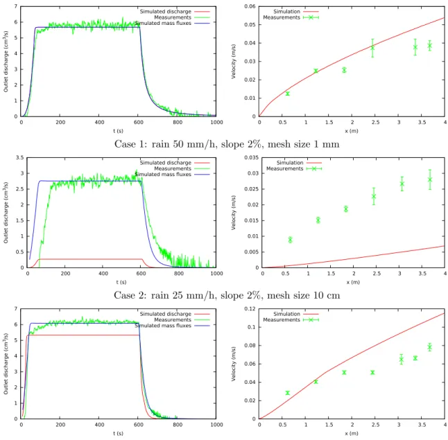
In the previous section, the numerical experiments show that our new model (2.4) with the additional friction coefficient to represent the furrows gives good results on the water

On the other hand, the Criel s/mer rock-fall may be linked to marine action at the toe of the cliff, because the water level reaches the toe of the cliff at high tide and the

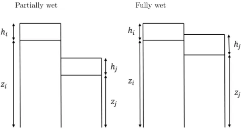
D’après les tableaux (Tableau 1 et Tableau 2), les résultats des deux méthodes de Saint Venant (version standard et version modifiée) pour le cas de sources profondes dans

Title Page Abstract Introduction Conclusions References Tables Figures J I J I Back Close Full Screen / Esc.. Print Version

Its contamination by a nematicide applied in banana cropping (Charlier et al, 2009, Journal of Environmental Quality, 38, 3, p.1031-1041) showed two successive phases, which

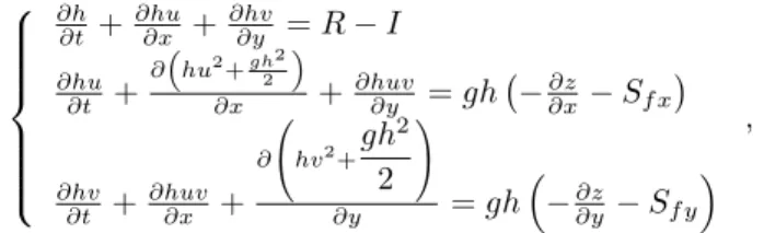
The aim of this note is to present a multi-dimensional numerical scheme approximating the solutions of the multilayer shallow water model in the low Froude number regime.. The