An Analytical Framework for the Steady State Impact of Carbonate Compensation on Atmospheric CO[subscript 2]

Carbonate Compensation on Atmospheric CO[subscript 2]

The MIT Faculty has made this article openly available.

Please share

how this access benefits you. Your story matters.

Citation

Omta, Anne Willem, Raffaele Ferrari, and David McGee. “An

Analytical Framework for the Steady State Impact of Carbonate

Compensation on Atmospheric CO[subscript 2].” Global

Biogeochemical Cycles 32, no. 4 (April 2018): 720–735.

As Published

http://dx.doi.org/10.1002/2017GB005809

Publisher

American Geophysical Union (AGU)

Version

Final published version

Citable link

http://hdl.handle.net/1721.1/120290

Terms of Use

Article is made available in accordance with the publisher's

policy and may be subject to US copyright law. Please refer to the

publisher's site for terms of use.

An Analytical Framework for the Steady State Impact

of Carbonate Compensation on Atmospheric CO

₂

Anne Willem Omta1 _{, Raffaele Ferrari}1_{, and David McGee}1

1_{Department of Earth, Atmospheric and Planetary Sciences, Massachusetts Institute of Technology, Cambridge, MA, USA}

Abstract

The deep-ocean carbonate ion concentration impacts the fraction of the marine calcium carbonate production that is buried in sediments. This gives rise to the carbonate compensation feedback, which is thought to restore the deep-ocean carbonate ion concentration on multimillennial timescales. We formulate an analytical framework to investigate the impact of carbonate compensation under various changes in the carbon cycle relevant for anthropogenic change and glacial cycles. Using this framework, we show that carbonate compensation amplifies by 15–20% changes in atmospheric CO2resulting from a redistribution of carbon between the atmosphere and ocean (e.g., due to changes in temperature, salinity, or nutrient utilization). A counterintuitive result emerges when the impact of organic matter burial in the ocean is examined. The organic matter burial first leads to a slight decrease in atmospheric CO₂and an increase in the deep-ocean carbonate ion concentration. Subsequently, enhanced calcium carbonate burial leads to outgassing of carbon from the ocean to the atmosphere, which is quantified by our framework. Results from simulations with a multibox model including the minor acids and bases important for the ocean-atmosphere exchange of carbon are consistent with our analytical predictions. We discuss the potential role of carbonate compensation in glacial-interglacial cycles as an example of how our theoretical framework may be applied.

1. Introduction

The partitioning of carbon between the ocean and the atmosphere is key for understanding glacial-interglacial changes in atmospheric CO₂(Archer et al., 2000; Menviel et al., 2008; Omta et al., 2006), as well as for predicting the fate of anthropogenic CO₂(Archer, 2005; Archer et al., 2009; Montenegro et al., 2007). By combining carbon mass balances with carbonate chemistry, analytical expressions have been derived to describe the ocean-atmosphere partitioning of carbon on multicentennial to millennial timescales (d’Orgeville et al., 2011; Goodwin et al., 2007, 2008, 2009; Ito & Follows, 2005; Kwon et al., 2011; Marinov, Follows, et al., 2008; Marinov, Gnanadesikan, et al., 2008; Omta et al., 2010, 2011). In our view, the great benefit of this analytical approach is that it leads to a quantitative intuition for the system. With such a quan-titative intuition, it is easier to assess which mechanisms have the largest impact on the atmospheric and oceanic carbon budgets, before embarking on time-consuming simulations. Here we apply the analytical approach to mechanisms repartitioning carbon between the ocean and the atmosphere on multimillennial timescales.

On multimillennial timescales, the ocean-atmosphere partitioning of carbon interacts with the ocean alka-linity cycle. Essentially, ocean alkaalka-linity is the concentration of bases (e.g., CO2−

3 ) available to react with CO2 to form HCO−

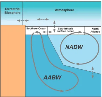
3. Alkalinity is transported into the ocean as a consequence of continental rock weathering and removed from the ocean through sedimentation and burial of calcifying organisms (see Figure 1). It is gener-ally assumed that the ocean maintains a balance between these input and output fluxes of alkalinity through a mechanism referred to as carbonate compensation, which works as follows. The CO2−

3 concentration ([CO 2− 3 ]) is lower in the deep ocean than at the surface, mainly because the soft-tissue carbon pump transfers carbon from the upper to the deep ocean (Volk & Hoffert, 1985). Furthermore, the solubility of calcium carbonate (CaCO3) increases with pressure (Pytkowicz & Conners, 1964). Due to a combination of these effects, much of the deep ocean is undersaturated with respect to calcite (Ridgwell & Zeebe, 2005). At a level named the car-bonate compensation depth (CCD), the rates of sedimentation and dissolution of calcite are equal. Below this level, there is no CaCO3present in sediments. A decrease of the deep-ocean [CO2−3 ] leads to an increase in both the dissolution of CaCO3from sediments and a decrease in the accumulation of new CaCO3sediments.

RESEARCH ARTICLE

10.1002/2017GB005809

Key Points:

• We formulate an analytical model for the ocean carbon cycle on multimillennial timescales • Carbonate compensation amplifies

by 15% changes in atmospheric CO2

due to changes in ocean temperature, salinity, or nutrient utilization • Organic matter burial in the ocean,

in combination with carbonate compensation, leads to outgassing of CO₂from the ocean to the atmosphere

Correspondence to:

A. W. Omta, omta@mit.edu

Citation:

Omta, A. W., Ferrari, R., & McGee, D. (2018). An analytical framework for the steady state impact of carbonate compensation on atmospheric CO₂. Global Biogeochemical Cycles, 32, 720–735. https://doi.org/10.1002/2017GB005809 Received 6 OCT 2017 Accepted 19 MAR 2018

Accepted article online 27 MAR 2018 Published online 26 APR 2018

©2018. American Geophysical Union. All Rights Reserved.

Figure 1. A schematic depiction of the input and output of alkalinity into and out of the ocean (figure adapted from

Omta et al., 2013). Alkalinity is added to the ocean through river runoff and is consumed by calcifiers and removed from the ocean through calcifier sedimentation. Above the carbonate compensation depth (CCD), calcium carbonate accumulates, whereas it dissolves below the CCD. A decrease in deep-ocean [CO2−

3 ] leads to a decrease in CaCO3output

and, thus, an increase in deep-ocean [CO2−₃ ]. This carbonate compensation feedback is thought to return the deep-ocean [CO2−

3 ] to its equilibrium value on a multimillennial timescale. This, in turn, leads to an increase in the deep-ocean [CO2−

3 ]. Overall, the deep-ocean [CO 2−

3 ] is expected to relax back to its original value, as long as the alkalinity input into the ocean by, for example, rivers does not change (Archer & Maier-Reimer, 1994; Sigman et al., 1998). The increased sediment dissolution and the decreased sediment accumulation mechanisms occur on two different timescales (Archer et al., 1997, 1998; Ridgwell & Hargreaves, 2007). Based on a suite of carbon release experiments with the carbon-centric Grid ENabled Integrated Earth system model (cGENIE), Lord et al. (2016) combined these two timescales into a single response time of 4–16 kyr (depending on the total carbon emissions). However, as a result of continuous equi-libration and reequiequi-libration of carbon between the atmosphere, ocean, and sediments, the overall relaxation has a long tail stretching tens of thousands of years.

Running numerical simulations for tens of thousands of years until full carbonate compensation has been achieved is very time consuming. Thus, simple analytical expressions for estimating the impact of carbon-ate compensation on atmospheric CO2are very useful, particularly if various different disturbances are to be investigated. Using the argument that [CO2−

3 ] returns to its original value, Goodwin and Ridgwell (2010) derived such an expression for the ocean-atmosphere partitioning of anthropogenic carbon on multimillen-nial timescales. From this expression, Goodwin and Ridgwell (2010) estimated that between 6% and 10% of anthropogenic carbon will remain in the atmosphere after carbonate compensation has been completed. We extend their work by deriving analytical expressions to estimate the overall impact of carbonate com-pensation in response to variations in ocean temperature, salinity, and nutrient utilization and the total ocean nutrient inventory (section 2). We compare the main predictions from our analytical framework against simulations with a multibox model including the full set of compounds involved in the ocean-atmosphere exchange of carbon, which is described in detail in Appendix A. We believe that the expressions derived here will be useful both for understanding how future climate change may feed back onto the marine carbon cycle and for understanding glacial-interglacial CO₂changes. We provide a more detailed discussion of the potential relevance of our findings for the future and the past carbon cycle in sections 3 and 4.

2. Analytical Framework

We start from a balance equation for carbon in the ocean-atmosphere system (Ito & Follows, 2005; Williams & Follows, 2011):

with M the total gas content of the atmosphere (mol), V the volume of the ocean (m3_{), X}

CO2the atmospheric

CO2mixing ratio (ppmv), and Ioathe total carbon inventory of the ocean-atmosphere system (mol). Csat, Creg, and Ccarb(all in mol/m3) describe the partitioning of dissolved inorganic carbon (DIC) into the different carbon pumps introduced by Volk and Hoffert (1985). Csatis the average oceanic saturated carbon concen-tration, which is somewhat higher than the average saturated carbon concentration at the ocean surface as a result of the lower temperature of the deep ocean (the solubility pump), Cregis the average regenerated carbon concentration (the soft-tissue pump), and Ccarbis the carbon added to the ocean through dissolution of sinking CaCO3(the carbonate pump).

The process of carbonate compensation leads to a change in the total carbon inventory of the ocean-atmosphere system because of the dissolution and burial of CaCO3. We will refer to such changes in Ioa as𝛿Ioa_,calc. Furthermore, carbon can be added or removed from the ocean-atmosphere system in forms other than CaCO3, for example, through anthropogenic carbon emissions and burial of particulate organic carbon (POC). We will refer to such changes in Ioaas𝛿Ioa,noncalc. Equation (1) can be used to relate the changes in the

total carbon inventory to changes in XCO2, Csat, Creg, and Ccarb:

M𝛿XCO₂+ V𝛿(Csat+ Creg+ Ccarb )

=𝛿Ioa_,calc+𝛿Ioa_,noncalc (2)

For every mole of carbon in CaCO₃that is added, the ocean gains two moles of alkalinity. Thus,𝛿Ioa_,calc =

V𝛿A

2 , with A the alkalinity. Furthermore, if we neglect the contributions to alkalinity from all acids and bases other than HCO−

3and CO 2−

3 , then𝛿A ≈ 𝛿[HCO − 3]+2𝛿[CO

2−

3 ]. Neglecting dissolved CO2,𝛿 (

Csat+ Creg+ Ccarb ) ≈ 𝛿[HCO− 3]+𝛿[CO 2− 3 ]. Hence,𝛿A ≈ 𝛿 (

Csat+ Creg+ Ccarb )

+𝛿[CO2− 3 ].

Following earlier analytical work on the impact of carbonate compensation (Goodwin & Ridgwell, 2010), the difference between the whole-ocean and deep-ocean average [CO2−

3 ] is neglected. The underlying assump-tion is that DIC and alkalinity are vertically homogeneous throughout most of the ocean. This seems a reasonable approximation for the current ocean, in which vertical gradients in DIC and alkalinity are rather small below ∼1,000 m (Chester, 2000). With this assumption (discussed in more detail in section 3.1), we can equate the whole-ocean average [CO2−

3 ] to the [CO 2−

3 ] at the CCD, relevant for carbonate compensation. Thus, we state that𝛿[CO2−

3 ] = 0 after full carbonate compensation, which means that𝛿A ≈ 𝛿 (

C_sat+ C_reg+ C_carb). Altogether, this gives

M𝛿XCO₂+V𝛿 (

Csat+ Creg+ Ccarb )

2 =𝛿Ioa,noncalc (3) Essentially, the term V𝛿(Csat+ Creg+ Ccarb

)

in equation (1) has been replaced in equation (3) by a term

V𝛿(Csat+Creg+Ccarb)

2 . The factor 1

2expresses that any transfer of carbon between the atmosphere and ocean will account for the full change in atmospheric carbon but only half of the change in oceanic carbon. This reflects the very nature of the carbonate compensation process: for every CO2molecule that the ocean takes up, the ocean also needs to take up a CO2−

3 ion from the sediment to restore the original [CO 2−

3 ]. This is an approxima-tion, because CO2−

3 and CO2also react with minor acids and bases, such as the boron species, H+, and OH−. However, it appears to be sufficiently accurate for our purposes, as we demonstrate in sections 2.1 and 2.2 through comparisons between our analytical predictions and simulations with a multibox model that includes these minor acids and bases.

In section 2.1, we derive an expression for the change in atmospheric CO2, if carbon is redistributed within the ocean-atmosphere system. In other words, we assume:𝛿Ioa_,noncalc= 0. Such a carbon redistribution could be due to a change in ocean temperature or salinity or a change in nutrient utilization. Without carbonate compensation, there would be no change in the total ocean-atmosphere carbon inventory, but the carbonate compensation process leads to input or output of carbon in the form of CaCO3. In section 2.2, we derive an expression for the change in atmospheric CO2, if some POC is buried instead of being remineralized in the water column. In other words:𝛿Ioa_,noncalc = 𝛿Ioa_,bur. To maintain deep-ocean [CO2−

3 ] at its original value, Creg and CaCO₃need to be removed in a 1:1 ratio. The resulting alkalinity decrease then leads to outgassing of CO₂ from the ocean to the atmosphere.

2.1. Carbonate Compensation in Response to Redistribution of Carbon in the Ocean-Atmosphere System

If the only changes in the total carbon inventory in the ocean-atmosphere system are due to the carbonate compensation process, then equation (3) becomes

M𝛿XCO₂+V𝛿 (

Csat+ Creg+ Ccarb )

2 = 0 (4)

The saturated carbon concentration is determined by the atmospheric CO2content and by the ocean tem-perature, salinity, and alkalinity. As in Goodwin and Lenton (2009), we split the dependencies of Csat into contributions from atmospheric CO2, temperature, alkalinity, and salinity, with B≡

𝜕lnX_CO2

𝜕lnCsat the Revelle buffer

factor (Bolin & Eriksson, 1959),𝛾T ≡ 𝜕C_𝜕Tsat,𝛾S ≡ 𝜕C_𝜕Ssat, and𝛾A ≡ 𝜕C_𝜕Asat. The change in ocean alkalinity (𝛿A) is

divided into a change in preformed alkalinity (𝛿Apref), relevant for the ocean-atmosphere carbon partitioning, a change due to the carbonate pump (𝛿Acarb= 2𝛿Ccarb) and a change due to the remineralization of organic matter (Sarmiento & Gruber, 2006) (𝛿Areg = −R_N∶C𝛿Creg, with RN∶Cthe Redfield N:C ratio). The expansion of

𝛿Csatgives 𝛿Csat= Csat X_CO 2B 𝛿XCO2+𝛾T𝛿T + 𝛾S𝛿S + 𝛾A𝛿Apref = Csat X_CO 2B 𝛿XCO2+𝛾T𝛿T + 𝛾S𝛿S + 𝛾A𝛿 ( A − Acarb− Areg ) = Csat X_CO 2B 𝛿XCO2+𝛾T𝛿T + 𝛾S𝛿S + 𝛾A𝛿 (

Csat+ Creg+ Ccarb )

+𝛾_A(R_N∶C𝛿Creg− 2𝛿Ccarb) (5)

which can be rearranged thus:

𝛿(Csat+ Creg+ Ccarb ) = Csat X_CO2B𝛿XCO2+𝛾T𝛿T + 𝛾S𝛿S + ( 1 + R_N∶C)𝛿Creg−(2𝛾_A− 1)𝛿Ccarb 1 −𝛾_A (6)

Substituting equation (6) into (4), we obtain ( 1 −𝛾A ) M𝛿XCO₂ = −V 2 ( Csat X_CO 2B 𝛿XCO2+𝛾T𝛿T + 𝛾S𝛿S + ( 1 + RN∶C ) 𝛿Creg− (2𝛾_A− 1)𝛿Ccarb ) (7) which can be used to calculate the change in atmospheric X_CO2:

𝛿XCO2= − 𝛾T𝛿T + 𝛾S𝛿S + ( 1 + R_N∶C)𝛿Creg−(2𝛾_A− 1)𝛿Ccarb 2(1 −𝛾A )M V + Csat X_CO2B (8)

This is the change in atmospheric XCO2after carbonate compensation resulting from a change in ocean

tem-perature (𝛿T), salinity (𝛿S), nutrient utilization (𝛿Creg), or the carbonate pump (𝛿Ccarb). Combining equation (8) with the balance equation (4) and𝛿A ≈ 𝛿(C_sat+ C_reg+ C_carb), the result can also be expressed in terms of whole-ocean alkalinity: 𝛿A = −2M𝛿XCO2 V = 𝛾T𝛿T + 𝛾S𝛿S + ( 1 + RN∶C ) 𝛿Creg−(2𝛾A− 1 ) 𝛿Ccarb 1 −𝛾A+ Csat X_CO2B V 2M (9)

Without carbonate compensation, the change in XCO2would be

𝛿XCO2= − 𝛾T𝛿T + 𝛾S𝛿S + ( 1 + RN∶C ) 𝛿Creg−(2𝛾A− 1 ) 𝛿Ccarb M V + Csat X_CO2B (10)

which is essentially a restatement of results derived in various earlier papers (Goodwin et al., 2008, 2011; Marinov, Follows, et al., 2008; Marinov, Gnanadesikan, et al., 2008; Omta et al., 2011).

The ratio of𝛿XCO₂with carbonate compensation to𝛿XCO₂without carbonate compensation is thus 𝛿XCO2(carbocomp.) 𝛿XCO2(nocarbocomp.) = MXCO2 +VCsat B 2(1 −𝛾A ) MXCO2+ VCsat B (11) Using M = 1.80×1020_{mol, X} CO2= 300 ppmv, V = 1.40×10 18_m3_,𝛾

A= 0.90, Csat= 2.00 mol/m3, and B = 12.0,

we get

𝛿XCO2(carbocomp.)

𝛿XCO2(nocarbocomp.)

≈ 1.18 (12)

That is, carbonate compensation enhances the change in atmospheric CO₂by about 18% after a redistribution of carbon between the atmosphere and the ocean. This value must have varied in the geological past, in particular because there have been variations in X_CO2.

To test this prediction of an ∼18% enhancement of CO2changes against more precise calculations including the minor acids and bases important for the ocean-atmosphere exchange of carbon (the boron species, H+_, and OH−_{), we use the multibox model described in Appendix A. The response of the ocean-atmosphere} car-bon partitioning to a perturbation in ocean temperature, salinity, or carcar-bon pumps is expected to occur on three timescales (Lord et al., 2016): (1) a multicentennial equilibration of carbon between the atmosphere and ocean, without significant interaction with the sediments; (2) a multimillennial equilibration with the calcite sediments through the carbonate compensation feedback; and (3) a final equilibration of the ocean alkalin-ity cycle due to adjustments in the silicate weathering rate on timescales of many hundreds of thousands of years.

In the simulations, we study the XCO2 response to perturbations in the ocean on the first two of these

timescales, neglecting long-term changes in the silicate weathering rate. First, we let the box model equi-librate on the faster timescale without carbonate compensation, after which we turn on the carbonate compensation to study the slower equilibration through the carbonate compensation feedback. In our multi-box model, the carbonate compensation process is formulated as a linear relaxation toward an equilibrium deep-ocean [CO2−

3 ] with a 5 kyr time constant.

The model is spun up for 200 kyr to equilibration with carbonate compensation switched on. With the imposed equilibrium deep-ocean [CO2−

3 ], ocean temperatures, and carbon and phosphorus inventories, the steady state XCO2 settles at 297 ppmv. Subsequently, we run a set of experiments in which the temperature of all

the ocean surface boxes is changed, with and without carbonate compensation. As expected, a temperature change has a somewhat stronger impact on atmospheric CO2with carbonate compensation than without it (Figure 2). The ratio_𝛿X𝛿XCO2(carbocomp.)

CO2(nocarbocomp.)increases from 1.15 to 1.21, as the imposed temperature change increases

from −5 to +5 ∘C (Figure 2b), which can be understood as follows. Since 2(1−𝛾A) is only about 0.2, equation (11)

can be approximated as 𝛿XCO2(carbocomp.)

𝛿X_CO2(nocarbocomp.) ≈ MX_CO2B

VCsat

+ 1. As X_CO2increases with increasing temperature,VCsat

B

remains relatively constant, which leads to the overall increase in the ratio.

To give an idea of the transient dynamics with and without carbonate compensation, we show full time series of XCO2, as well as DIC and alkalinity in the Antarctic Bottom Water (AABW) box. First, the sea surface

tempera-tures (SST) are decreased by 5 ∘C without carbonate compensation (Figure 3). The temperature change leads to a repartitioning of carbon between the atmosphere and the ocean: XCO2decreases by 48 ppmv (green line

in Figure 3a), while DIC increases by 7 μM (green line in Figure 3b). The alkalinity remains constant, as long as there is no carbonate compensation (green line in Figure 3c). After 10 kyr, the system has equilibrated and we switch the carbonate compensation on, while the low SST are maintained. The carbonate compensation pro-cess leads to a further decrease in atmospheric X_CO2of just over 7 ppmv (blue line in Figure 3a), an increase in DIC of 9 μM (blue line in Figure 3b), and an increase in alkalinity of 16 μM (blue line in Figure 3c). This is slightly more than the alkalinity change expected from our framework:𝛿A = −2M𝛿X_VCO2=14 μM, which is likely due to the contributions from minor acids and bases such as the boron species. The carbonate compensa-tion takes place on a timescale much longer than the imposed 5 kyr response time because of the asymptotic nature of the overall equilibration process. That is, a certain change in temperature leads to a certain change

Figure 2. (a) Atmospheric CO₂as a function of the change in global mean sea surface temperature (SST), after a 250 kyr equilibration with carbonate compensation (blue diamonds) and without carbonate compensation (red squares). The green diamond indicates the spin-up simulation; the black crosses indicate the simulation experiment shown in Figure 3. (b) The ratio_𝛿X𝛿XCO2(carbocomp.)

CO2(nocarbocomp.) as a function of the change in global mean SST; again, the black cross indicates the simulation experiment shown in Figure 3.

in X_CO2and deep-ocean DIC. This leads to CaCO₃dissolution or burial, which in turn leads to a change in atmo-spheric X_CO2, which in turn leads to CaCO₃dissolution or burial, which in turn leads to a change in atmospheric X_CO2, etc.

2.2. Carbonate Compensation in Response to Organic Matter Burial

If organic carbon and phosphorus are buried instead of being remineralized, then there is a decrease in the inventory of regenerated carbon equal to the decrease in the total carbon inventory:𝛿Ioa_,noncalc= 𝛿Ioa_,bur = V𝛿Creg. In this case, equation (3) becomes

M𝛿XCO₂+V𝛿 (

Csat+ Creg+ Ccarb )

2 = V𝛿Creg (13)

or

M𝛿XCO₂+V𝛿 (

Csat− Creg+ Ccarb )

2 = 0 (14)

We use an expansion analogous to equation (5) but ignoring any changes in the temperature and salinity, because the focus is on changes in the nutrient inventory:

𝛿(C_sat− C_reg+ C_carb)= Csat XCO2B

𝛿XCO2

Figure 3. Multibox model simulation: after the spin-up (red line), the sea surface temperature is decreased by 5∘C everywhere, first without carbonate compensation (green line) and finally with carbonate compensation (blue line); (a) atmospheric CO₂, (b) dissolved inorganic carbon (DIC) in the Antarctic Bottom Water box, and (c) total alkalinity in the Antarctic Bottom Water box.

Collecting𝛿(Csat− Creg+ Ccarb )

terms on the left-hand side and dividing by 1 −𝛾Agives

𝛿(Csat− Creg+ Ccarb ) = Csat X_CO2B𝛿XCO2 ( 2𝛾_A− 1 + R_N∶C)𝛿Creg−(2𝛾_A− 1)𝛿Ccarb 1 −𝛾_A (16)

Combining equations (14) and (16) then leads to

𝛿XCO2= − ( 2𝛾A− 1 + RN∶C ) 𝛿Creg−(2𝛾A− 1 ) 𝛿Ccarb 2(1 −𝛾_A)M V + Csat X_CO2B (17)

Equation (17), which describes the impact of burial of POC on𝛿XCO₂, is identical to equation (8), which applies to a change in nutrient utilization (setting𝛿T and 𝛿S equal to 0), except that the factor 1+RN∶Cin front of𝛿Creg

is replaced by 2𝛾A− 1 + RN∶C. Given that

2𝛾A−1+RN∶C

1+RN∶C

≈ 0.8, the change in atmospheric CO2after carbonate com-pensation is ∼20% smaller if it is caused by POC burial than if it is caused by a decreased nutrient utilization, for a given decrease in the regenerated carbon𝛿Creg.

Using equation (13) and𝛿A ≈ 𝛿(C_sat+ C_reg+ C_carb), equation (17) can also be cast as an expression for the whole-ocean alkalinity change:

𝛿A = 2 ( −M𝛿XCO2 V +𝛿Creg ) = ( 2𝛾A− 1 + RN∶C ) 𝛿Creg−(2𝛾A− 1 ) 𝛿Ccarb 1 −𝛾A+ Csat X_CO2B V 2M + 2𝛿Creg (18)

The sinkings of POC and CaCO3are intimately connected with each other (Klaas & Archer, 2002). Consistently, we assume that the whole-ocean average strengths of the carbonate pump and the soft-tissue pump

Figure 4. Atmospheric CO₂as a function of the total amount of buried particulate organic carbon (POC), after a 250-kyr equilibration with carbonate compensation (blue diamonds). The green diamond indicates the spin-up simulation; the black cross stands for the simulation experiment shown in Figure 5. The red line indicates the slope predicted by relation (19), usingM = 1.80 × 1020mol,X_CO2= 300ppmv,V = 1.40 × 1018m3,𝛾_A= 0.90, C_sat= 2.00mol/m3_{,B = 12.0, andR}

calc= 0.100. In calculating this slope,

the alkalinity change directly resulting from the remineralization of organic matter (_𝛿Areg= −RN∶C𝛿Creg) was neglected, because this effect is not

included in our multibox model.

are proportional to each other: Ccarb= RcalcCreg(with Rcalcthe whole-ocean average ratio of CaCO3:organic carbon added to the water column). If using an average Rcalcvalue for the whole ocean is a valid approximation, then equation (17) can be rewritten as

𝛿XCO2= − ( (2𝛾_A− 1)(1 − R_calc) + R_N∶C)𝛿Creg 2(1 −𝛾A )M V + Csat X_CO2B (19)

The ratio Rcalcdetermines to what extent the carbonate compensation in the deep ocean is communicated to the ocean surface. If this ratio were 1:1, then the weakening of the soft-tissue carbon pump and the associated carbonate compensation would be offset exactly by a weakening of the carbonate pump, and [CO2−

3 ] at the ocean surface (and thus atmospheric CO2) would remain constant. However, the average ratio of CaCO3:POC added to the water column is believed to be in the 0.1–0.2:1 range (Boyle, 1988; Yamanaka & Tajika, 1996). Hence, a large fraction of the alkalinity output in the deep ocean is communicated to the surface ocean, because less carbon is added to the deep ocean through the carbonate pump than through the soft-tissue carbon pump.

To test equation (19), we again use our multibox model. In all the simu-lations, POC and organic phosphorus are exported from the surface in a fixed Redfield ratio of 106:1. After the 200-kyr spin-up during which all the exported POC and phosphorus are remineralized in the deep ocean, we switch on the burial. During 10 kyr, a fraction of the exported carbon and phosphorus is taken out of the ocean-atmosphere system in the 106:1 Redfield ratio instead of being rem-ineralized, which reduces the strength of the soft-tissue carbon pump. Subsequently, the burial is switched

Figure 5. Multibox model simulation: after the spin-up (red line), organic carbon and phosphorus are buried (green

line). Most of the carbonate compensation takes place after the burial has been halted (blue line). (a) Atmospheric CO₂, (b) dissolved inorganic carbon (DIC) in the Antarctic Bottom Water (AABW) box, (c) total alkalinity in the AABW box, and (d) dissolved inorganic phosphorus (DIP) in the AABW box.

off and the system is left to equilibrate. The carbonate compensation is switched on at all times. To vary the output of organic phosphorus and POC, we run a set of simulations where the burial fraction is increased from 0.2% to 2.0% in 0.2% increments. The total amount of phosphorus buried in the model experiments varied between 0.05 × 1015_{and 0.50 × 10}15_{mol, out of a total initial inventory of 2.41×10}15_{mol; the total amount of} POC buried varied between 70 Pg C and 630 Pg C. In Figure 4, we show atmospheric CO₂as a function of the total amount of buried POC, after full equilibration (250 kyr) with carbonate compensation, along with the slope predicted by relation (19). As can be seen, there is excellent agreement between the analytical theory and the box model simulations.

In Figure 5, we show the time series of XCO2, as well as DIC, alkalinity, and dissolved inorganic phosphorus in the

AABW box for one of the simulations. During the burial phase, there are two competing effects: the removal of phosphorus weakens the soft-tissue carbon pump and therefore increases atmospheric CO₂, whereas the removal of carbon decreases atmospheric CO₂. In our box model, the combined removal of carbon and phos-phorus under the Redfield ratio before significant carbonate compensation leads to a minor decrease in X_CO2 (green line in Figure 5a). (This reflects that there is not full nutrient utilization. With full nutrient utilization across the ocean (C_reg = R_C∶PP) and a removal of carbon and phosphorus according to the Redfield ratio (𝛿Ioa_,noncalc = R_C∶P𝛿P), then Ioa_,noncalc =𝛿Creg. That is, equation (2) becomes: M𝛿XCO₂+ V𝛿(C_sat+ C_carb) = 0. If C_carb does not change, then the net effect on atmospheric CO₂is 0, as C_satdepends only on X_CO2, tem-perature, salinity, and alkalinity.) During the burial phase, the major changes are in the ocean carbon and phosphorus inventories: DIC decreases by 27 μM (green line in Figure 5b), while the dissolved inorganic phosphorus concentration decreases by 0.22 μM (green line in Figure 5d). The alkalinity decrease is still rel-atively minor (green line in Figure 5c), because the carbonate compensation process responds to changes in the deep ocean [CO2−

3 ] with a lag of many thousands of years. After the burial phase, the carbonate com-pensation leads to a rather large increase in XCO2(blue line in Figure 5a), as well as major decreases in DIC

and alkalinity (blue lines in Figures 5b/c), while the dissolved inorganic phosphorus concentration remains constant (blue line in Figure 5d). The overall increase in XCO2 equals 24 ppmv, whereas the overall

alkalin-ity decrease equals 57 μM eq. Based on𝛿A = 2(−M𝛿XCO2

V +𝛿Creg

)

, one would expect an alkalinity decrease of 61 μM eq, under the assumption that𝛿Creg = R_C∶P𝛿P. Again, the final state is only achieved after many tens of thousands of years, during which there is continuous equilibration and reequilibration between the different reservoirs.

3. Discussion

As in section 2, we first discuss carbonate compensation under a constant nutrient inventory (section 3.1), before moving to the potential combined impact of POC burial and carbonate compensation (section 3.2). Finally, we discuss how CaCO3preservation and production may impact the timescale at which deep-ocean [CO2−

3 ] is restored (section 3.3).

3.1. Constant Nutrient Inventory

Our analytical framework (as well as our multibox model) predicts that carbonate compensation increases by 15–20% the impact of changes in atmospheric CO2resulting from a redistribution of carbon between the atmosphere and ocean. The full changes in atmospheric CO2due to variations in the ocean temperature and the soft-tissue carbon pump can thus be inferred from coupled ocean-atmosphere-biogeochemistry models that do not include carbonate compensation and are therefore cheaper to run, because they equilibrate in multicentennial timescales rather than multimillennial timescales. The rule of thumb is then to multiply the model’s predicted CO2changes by 1.15–1.20 to account for carbonate compensation.

The most important application of the 15–20% rule of thumb will likely be in the study of glacial-interglacial cycles. Ice core measurements suggest that atmospheric CO₂ dropped by 80–100 ppmv during glacial climates compared to interglacials (Lüthi et al., 2008; Petit et al., 1999). These drops may have involved vari-ous disturbances of the ocean carbon system (Chikamoto et al., 2012; Peacock et al., 2006; Wallmann, 2014), for example, changes in the whole-ocean temperature, salinity, alkalinity, and nutrient utilization. However, it remains unclear whether the net impact of all these ocean changes can amount to the total 80–100 ppmv swings in atmospheric CO2(Brovkin et al., 2012; Sigman & Boyle, 2000; Sigman et al., 2010). Our study suggests that changes in ocean temperature, salinity, alkalinity, and nutrient utilization need explain only 70–85 ppmv changes, because an additional 15–20% can be attributed to carbonate compensation.

Another important application of our result is to predict the long-term fate of anthropogenic carbon emis-sions, for which Goodwin and Ridgwell (2010) previously developed an analytical framework. They focused on the chemical processes (air-sea carbon partitioning and carbonate compensation) in isolation, without considering the impact of the changing climate on the ocean-atmosphere partitioning of CO₂. However, tem-perature is expected to change under global warming. Furthermore, it has been suggested that the soft-tissue carbon pump will strengthen in a high CO₂world (Bernardello et al., 2014; Oschlies et al., 2008; Riebesell et al., 2007). All these hypothesized mechanisms essentially involve a redistribution of carbon between the ocean and the atmosphere, which means that their impacts on atmospheric CO₂will be enhanced by 15–20% after carbonate compensation.

Our framework is built on an assumption that DIC and alkalinity are more or less vertically homogeneous throughout most of the ocean, which holds in the present-day ocean. The framework needs to be modified if there is a strong vertical heterogeneity in DIC at intermediate depths and in the abyss. In fact, this has already been demonstrated by earlier box model simulations (Hain et al., 2010). In these simulations, carbonate com-pensation enhanced the impact of changes in nutrient utilization on atmospheric CO2by 16% (i.e., within our predicted 15–20%) under the present-day ocean circulation. However, under an inferred glacial circulation, carbonate compensation enhanced the impact of changes in nutrient utilization on atmospheric CO2by 32%. This stronger carbonate compensation feedback was likely due to the “focusing” of regenerated nutrients and carbon in a water mass around the CCD. In the future, we plan to expand our framework with multiple water masses, so that, for example, the impact of nutrient focusing in an isolated reservoir can be considered.

3.2. Organic Matter Burial

Our analytical framework (as well as our multibox model) predicts that the combination of organic matter burial and carbonate compensation leads to an increase in atmospheric CO2. Although this result may seem counterintuitive, it can be understood intuitively as follows. After a mole of phosphorus has first become available for biological production, it provides for a net uptake of CO2from the atmosphere at two points in time: (1) the first time the mole of phosphorus is incorporated into organic matter and (2) the first time the mole of phosphorus, incorporated in organic matter, is remineralized in the deep ocean. At this point, DIC is released into the deep ocean, leading to a decrease in deep-ocean [CO2−

3 ], since𝛿[CO 2−

3 ] ≈𝛿A − 𝛿C. This, in turn, leads to a net dissolution of CaCO3and an ocean alkalinity increase. Once the ocean-atmosphere system has equilibrated, the alkalinity increase will have led to an uptake of CO2from the atmosphere into the ocean. When the mole of phosphorus is finally buried, the CO₂uptake achieved in step (1) is made permanent, while the step (2) CO₂uptake is reversed. The carbonate compensation proceeds in the other direction, leading to a decrease in ocean alkalinity and an outgassing of CO₂from the ocean into the atmosphere. This outgassing is expected to take place on the ∼4–16 kyr timescales associated with the equilibration of the sediments (Lord et al., 2016), with a long tail due to the continuing equilibration and reequilibration between the ocean and the atmosphere. Thus, the impact of organic matter burial depends on the timescale that one considers. The residence time of phosphorus in the ocean is estimated to be 10–40 kyr (Filippelli, 2011; Ruttenberg, 2003), which means that uptake in step (2) and its reversal can safely be neglected on timescales of millions of years but not on timescales of tens of thousands of years.

Could this mechanism have played a role in glacial-interglacial CO2changes? Broecker (1982) suggested that at the end of glacial-interglacial transitions, enhanced organic matter burial may have occurred on newly flooded continental shelves. However, Peacock et al. (2006) argued that this mechanism can only be respon-sible for a small portion of the deglacial weakening of the soft-tissue carbon pump, based on the thickness of the deglacial sediment cover on the Sunda Shelf—the world’s largest shallow shelf (Hanebuth et al., 2000). Moreover, Kohfeld and Ridgwell (2009) suggested that the deglacial sea level rise occurred too late for this mechanism to have played a major role in the deglacial rise in atmospheric CO2. The continental shelves only flooded toward the end of the deglaciation, after the main Northern Hemisphere ice sheets had melted, and the carbonate compensation process would have taken place even later. In response to both these objec-tions, we wish to point out that recent observations suggest that enhanced deglacial productivity may have occurred in the open ocean, rather than on newly flooded continental shelves. In fact, deglacial maxima in productivity proxies such as opal accumulation and biogenic Ba have been found at deep-sea sites in the Atlantic (Gil et al., 2009; Meckler et al., 2013; Romero et al., 2008), the Pacific (Galbraith et al., 2007; Hayes et al., 2011; Jaccard et al., 2005; Kohfeld & Chase, 2011), and the Southern Ocean (Anderson et al., 2009; Jaccard et al., 2013). Although it remains difficult to quantify from these observations the total amount of organic matter

buried, together they suggest that the deglacial decrease of the ocean nutrient inventory could have been more significant than generally recognized.

3.3. Restoring Deep-Ocean [CO2−₃ ]: Preservation Versus Production

The assumption that the deep-ocean [CO2−

3 ] returns to its original value after a disturbance is key to the appli-cation of our framework. The geological record provides strong evidence for this assumption. Focusing on glacial-interglacial cycles, the B/Ca proxy indicates only small changes in the deep-ocean [CO2−

3 ] (in particular if averaged over different locations; Doss & Marchitto, 2013; Kerr et al., 2017; Raitzsch et al., 2011; Rickaby et al., 2010; Yu et al., 2010, 2014). That said, a study of 31 cores from the Pacific, Atlantic, and Indian Oceans specifically focused on CaCO3dissolution proxies (Mekik et al., 2012) did not find strong evidence for a global deglacial carbonate preservation maximum, which presents somewhat of a mystery from the conventional carbonate compensation perspective.

Perhaps, the focus has been too much on CaCO3dissolution and preservation: a large net deglacial CaCO3 accumulation could also be achieved through an increase in CaCO3production. For example, a deglacial max-imum in organic matter production would likely have been accompanied by a deglacial maxmax-imum in CaCO₃ production. Due to POC being remineralized at faster rates than CaCO3, the global average CaCO3:POC ratio of material collected in sediment traps at depths below ∼1,000 m is close to 1:1 (Figure 4c in Archer, 1996), which implies an output of carbon and alkalinity in a ∼1:1 ratio. If this ratio applied during a deglacial burial event, then the organic matter burial and the alkalinity output needed to maintain a constant whole-ocean [CO2−

3 ] would have occurred simultaneously (since𝛿[CO 2−

3 ] ≈𝛿A − 𝛿C). Thus, a combined burial of POC and CaCO3would have accelerated the carbonate compensation process. From this perspective, it is interesting that the deglacial oceanic productivity maximum appears to be accompanied by a maximum in the CaCO₃ fraction of the sediments (Brunelle et al., 2010; Flores et al., 2003; Gebhardt et al., 2008; Jaccard et al., 2005; Jaccard et al., 2013; Rickaby et al., 2010). Enhanced CaCO3production is a particularly viable explanation for deglacial CaCO₃maxima at locations with continuous CaCO₃accumulation, such as the Cape Basin (Flores et al., 2003) and the Weddell Sea (Rickaby et al., 2010). However, even at locations without continuous CaCO3 accumulation (e.g., the deep North Pacific, Jaccard et al., 2005; and the deep Southern Ocean, Jaccard et al., 2013) where deglacial CaCO3spikes represent transient deepenings of the CCD, these CCD deepenings could ultimately be driven by CaCO3production. The CCD is the level where the supply and dissolution of CaCO3 are equal. Hence, the CCD deepens when the CaCO3supply increases, even if the CaCO3dissolution rate remains constant.

4. Conclusions

We have created an analytical framework for quantifying the impacts on atmospheric CO2of various carbon cycle disturbances after carbonate compensation has been completed. We think that a few points are crucial: 1. Carbonate compensation amplifies by ∼15–20% changes in atmospheric CO2resulting from

redistribu-tion of carbon within the ocean-atmosphere system (due to changes in temperature, salinity, and nutrient utilization).

2. Counterintuitively, the combination of organic matter burial in the ocean and carbonate compensation leads to an increase in atmospheric CO2. According to our framework, changes in the soft-tissue carbon pump have very similar impacts on atmospheric CO₂after carbonate compensation, regardless of their origin. That is, burial of 10% of the nutrient inventory has almost the same impact as a 10% decrease in the nutrient utilization.

3. The impact of carbonate compensation on atmospheric CO₂predicted from our analytical theory is consis-tent with multibox model calculations involving the full set of reactions involved in the ocean-atmosphere exchange of carbon, including the boron species, H+_{, and OH}−_.

In the near future, we intend to apply our framework to investigate hypotheses about the glacial-interglacial CO2 changes quantitatively. However, our framework can also be used to assess the long-term fate of anthropogenic CO2.

Appendix A: Multibox Setup

The multibox model was modified from an earlier version used in Omta et al. (2013, 2016). The initial tracer concentrations are listed in Table A1, along with their respective values at the end of the spin-up. In Table A2, the model parameters (e.g., box volumes and transport rates) and their respective values are listed.

Table A1

Description of Multibox Model Variables, With Their Respective Meanings, Units, and Values at the End of the Spin-Up

Variables Units Meaning Initial value Value after spin-up

A_s mol eq/m3 _{Southern Ocean alkalinity 2.200 2.260}

A_l mol eq/m3 _{Low-latitude alkalinity 2.200 2.227}

A_n mol eq/m3 North Atlantic alkalinity 2.200 2.221

A_i mol eq/m3 _{NADW alkalinity 2.400 2.235}

Ad mol eq/m3 AABW alkalinity 2.400 2.363

C_s mol/m3 _{Southern Ocean DIC concentration 2.160 2.095}

C_l mol/m3 _{Low-latitude DIC concentration 2.160 1.958}

C_n mol/m3 _{North Atlantic DIC 2.160 2.040}

C_i mol/m3 _{NADW DIC concentration 2.350 2.249}

C_d mol/m3 AABW DIC concentration 2.350 2.353

P_s mol eq/m3 _{Southern Ocean phosphorus concentration 5.000 × 10}−5 _{8.338 × 10}−5

Pl mol eq/m3 Low-latitude phosphorus concentration 5.000 × 10−5 0.9059 × 10−5

P_n mol eq/m3 _{North Atlantic phosphorus concentration 5.000 × 10}−5 _{4.564 × 10}−5

P_i mol eq/m3 _{NADW phosphorus 2.000 × 10}−3 _{1.934 × 10}−3

P_d mM AABW phosphorus 2.000 × 10−3 _{2.068 × 10}−3

X_CO

2 ppmv Atmospheric CO2mixing ratio 200.0 296.6

Notes. NADW = North Atlantic Deep Water; AABW = Antarctic Bottom Water; DIC = dissolved inorganic carbon.

Table A2

Description of Multibox Model Parameters (Par), With Their Respective Units, Meanings, and Values

Par Units Meaning Standard value

Vol_s m3 Southern Ocean surface box volume 4.2 × 1016

Vol_l m3 _{Low-latitude surface box volume 6.0 × 10}16

Voln m3 North Atlantic surface box volume 1.8 × 1016

Vol_i m3 _{NADW box volume 6.0 × 10}17

Vol_d m3 _{AABW box volume 6.0 × 10}17

M mol Amount of gas in atmosphere 1.8 × 1020

V_p m/s Piston velocity 5_{.0 × 10}−5

m_sl Sv Bidirectional mixing between Southern Ocean and low-latitude boxes 20.0

m_lh Sv Bidirectional mixing between low-latitude and North Atlantic boxes 20.0

mhi Sv Bidirectional mixing between NADW and North Atlantic boxes 10.0

m_id Sv Bidirectional mixing between NADW and AABW boxes 2.0

m_li Sv Bidirectional mixing between NADW and low-latitude boxes 2.0

m_si Sv Bidirectional mixing between Southern Ocean and NADW boxes 5.0

q_n Sv NADW overturning transport 15.0

q_s Sv AABW overturning transport 15.0

R_C∶P – Carbon:phosphorus ratio soft tissue 106

Rcalc – Inorganic:organic carbon ratio of remineralization 0.1

T_s ∘C Southern Ocean temperature 3

T_l ∘C Low-latitude box temperature 20

T_d ∘C North Atlantic temperature 5

𝜆s s−1 Southern Ocean export rate 1.07 × 10−8

𝜆l s−1 Low-latitude export rate 6.43 × 10−8

𝜆n s−1 North Atlantic export rate 2.14 × 10−8

[CO2−₃ ]eq mol/m3 Equilibrium [CO2−3 ] in the AABW box 0.01

𝜏 kyr Carbonate compensation time 5.0

Figure A1. A schematic depiction of the multibox setup; box volumes, transport rates, and tracer concentrations before

and after the spin-up are listed in Tables A1 and A2.

There are well-mixed atmospheric, low-latitude surface ocean, North Atlantic surface ocean, Southern Ocean surface, North Atlantic Deep Water (NADW), and Antarctic Bottom Water (AABW) boxes (Figure A1). A terres-trial biosphere compartment is also included in the model, but the size of this compartment is kept constant in the simulations. For the oceanic boxes, tracer concentrations are calculated through three modules: ocean-atmosphere carbon exchange, carbon isotope partitioning, and oceanic transport. For each surface ocean box, the carbon exchange module calculates the oceanic XCO2using DIC, alkalinity, and the water

tem-perature of the box by solving the full carbonate system with the Follows et al. (2006) scheme. Then, the air-sea flux of carbon𝜙 between the box and the atmosphere is calculated from the difference between XCO_2,oce and XCO_2,atm:

𝜙 = Vpak0(XCO_2,atm− XCO_2,oce) (A1) with Vpthe piston velocity and ak0an equilibrium constant. Tracers are exchanged between the oceanic boxes through bidirectional mixing between boxes j and k with volumes Voljand Volkat rates mjkand through

over-turning transports qn(NADW) and qs(AABW). For each tracer Y, it consists of the following equations (with the

subscripts n, l, s, i, and d indicating the North Atlantic surface, low-latitude surface, Southern Ocean surface, NADW, and AABW boxes, respectively):

𝜕Yn 𝜕t = −(q_n+ m_lh)(Y_n− Y_l) − m_hi(Y_n− Y_i) Voln (A2) 𝜕Yl 𝜕t = −(q_n+ m_li)(Y_l− Y_i) − m_ln(Y_l− Y_n) − m_ls(Y_l− Y_s) Voll (A3) 𝜕Ys 𝜕t = −q_s(Y_s− Y_d) − m_si(Y_s− Y_i) − m_ls(Y_s− Y_l) Vol_s (A4) 𝜕Yi 𝜕t = −(q_n+ m_hi)(Y_i− Y_h) − m_id(Y_i− Y_d) − m_li(Y_i− Y_l) Voli (A5) 𝜕Yd 𝜕t = −q_s(Y_d− Y_s) − m_id(Y_d− Y_i) Vol_d (A6)

We assume that dissolved inorganic phosphorus is the limiting nutrient. To represent the soft-tissue carbon pump, phosphorus is taken out of the surface boxes at rates𝜆_jfrom the surface boxes (as in Zhang et al., 2001), along with carbon through a constant Redfield ratio (R_C∶P= 106). The carbonate pump is represented through a constant CaCO₃:POC ratio of the exported carbon (R_calc= 0.1). The exported phosphorus, carbon, and alkalinity are added to the deep boxes, with one third going to the AABW box and two thirds going to the NADW box; no burial of organic matter takes place in the standard setup. Following various earlier studies (Boudreau, 2013; Boyle, 1983; Broecker & Peng, 1982; Köhler et al., 2010), the carbonate compensation feedback is formulated as a linear relaxation toward an equilibrium carbonate ion concentration ([CO2−

3 ]eq) in the deep (AABW) box:

𝜕Cd dt = − Ad− Cd− [CO2−3 ]eq 𝜏 (A7) 𝜕Ad dt = −2 Ad− Cd− [CO2−3 ]eq 𝜏 (A8) in which [CO2−

3 ]dis approximated as Ad− Cd. We choose a response time𝜏 = 5 kyr, because recent simulations

with the Grid Enabled Integrated Earth system model (GENIE) have indicated that the effective carbonate compensation timescale is ∼5 kyr for relatively small total carbon emissions of ∼1,000 Pg (Lord et al., 2016). These emissions are of a similar order of magnitude as the amounts of carbon that are exchanged between different reservoirs before carbonate compensation in the situations under consideration (0–100 Pg in the temperature change experiments and 0–700 Pg in the carbon burial experiments).

References

Anderson, R. F., Ali, S., Bradtmiller, L. I., Nielsen, S. H. H., Fleisher, M. Q., Anderson, B. E., & Burckle, L. H. (2009). Wind-driven upwelling in the Southern Ocean and the deglacial rise in atmospheric CO₂. Science, 323, 1443–1448.

Archer, D., Eby, M., Brovkin, V., Ridgwell, A., Cao, L., Mikolajewicz, U., et al. (2009). Atmospheric lifetime of fossil fuel carbon dioxide. Annual

Review of Earth and Planetary Science, 37, 117–134.

Archer, D. E. (1996). A data-driven model of the global calcite lysocline. Global Biogeochemical Cycles, 10, 511–526. https://doi.org/10.1029/96GB01521

Archer, D. E. (2005). Fate of fossil fuel CO2in geologic time. Journal of Geophysical Research, 110, C09S05. https://doi.org/10.1029/

2004JC002625

Archer, D. E., & Maier-Reimer, E. (1994). Effect of deep-sea sedimentary calcite preservation on atmospheric CO2concentration. Nature, 367,

260–264.

Archer, D. E., Kheshgi, H., & Maier-Reimer, E. (1997). Multiple timescales for neutralization of fossil fuel CO2. Geophysical Research Letters, 24,

405–408.

Archer, D. E., Kheshgi, H., & Maier-Reimer, E. (1998). Dynamics of fossil fuel CO₂neutralization by marine CaCO₃. Global Biogeochemical

Cycles, 12, 259–276.

Archer, D. E., Eshel, G., Winguth, A., Broecker, W., Pierrehumbert, R., Tobis, M., & Jacob, R. (2000). AtmosphericpCO₂sensitivity to the biological pump in the ocean. Global Biogeochemical Cycles, 14, 1219–1230.

Bernardello, R., Marinov, I., Palter, J. B., Sarmiento, J. L., Galbraith, E. D., & Slater, R. D. (2014). Response of the ocean natural carbon storage to projected twenty-first-century climate change. Journal of Climate, 27, 2033–2053.

Bolin, B., & Eriksson, E. (1959). Distribution of matter in the sea and the atmosphere. In B. Bolin (Ed.), The atmosphere and the sea in motion. New York: The Rockefeller Institute Press.

Boudreau, B. P. (2013). Carbonate dissolution rates at the deep ocean floor. Geophysical Research Letters, 40, 744–748.

Boyle, E. A. (1983). Chemical accumulation variations under the Peru current during the past 130,000 years. Journal of Geophysical Research,

88, 7667–7680.

Boyle, E. A. (1988). Vertical oceanic nutrient fractionation and glacial/interglacial CO₂cycles. Nature, 331, 55–56. Broecker, W. S. (1982). Ocean chemistry during glacial time. Geochimica et Cosmochimica Acta, 46, 1689–1705. Broecker, W. S., & Peng, T. H. (1982). Tracers in the Sea Lamont-Doherty Geological Observatory. Palisades: NY.

Brovkin, V., Ganopolski, A., Archer, D. E., & Munhoven, G. (2012). Glacial CO₂cycle as a succession of key physical and biogeochemical processes. Climate of the Past, 8, 251–264.

Brunelle, B. G., Sigman, D. M., Jaccard, S. L., Keigwin, L. D., Plessen, B., Schettler, G., et al. (2010). Glacial/interglacial changes in nutrient supply and stratification in the western subarctic North Pacific since the penultimate glacial maximum. Quaternary Science Reviews, 29, 2579–2590.

Chester, R. (2000). Marine geochemistry (2nd ed.). Oxford: Blackwell.

Chikamoto, M. O., Abe-Ouchi, A., Oka, A., Ohgaito, R., & Timmermann, A. (2012). Quantifying the ocean’s role in glacial CO₂reductions.

Climate of the Past, 8, 545–563.

d’Orgeville, M., England, M. H., & Sijp, W. P. (2011). Buffered versus non-buffered ocean carbon reservoir variations: Application to the sensitivity of atmosphericpCO,2to ocean circulation changes. Geophysical Research Letters, 38, L24603. https://doi.org/10.1029/

2011GL049823

Doss, W., & Marchitto, T. M. (2013). Glacial deep ocean sequestration of CO₂driven by the eastern equatorial Pacific biologic pump.

Earth and Planetary Science Letters, 377, 43–54.

Filippelli, G. M. (2011). Phosphate rock formation and marine phosphorus geochemistry: The deep time perspective. Chemosphere, 84, 759–766.

Acknowledgments

The authors would like to thank Mick Follows, Ros Rickaby, Ed Boyle, Andy Ridgwell, and an anonymous reviewer for helpful comments and inspiring discussions. Ian Hall created the schematic of the multibox model (Figure A1). The model code and output can be accessed through https://www.dropbox.com/sh/ m89mq7szcmwna8i/AADt1ACFvQJqDW u08CXQe5mOa?dl=0. AWO was supported by the Gordon and Betty Moore Foundation (grant GBMF 3778 awarded to Mick Follows) and the Simons Foundation (SCOPE award 329108, Follows). RF acknowledges NSF support through grant OCE-1536515.

Flores, J. A., Marino, M., Sierro, F. J., Hodell, D. A., & Charles, C. D. (2003). Calcareous plankton dissolution pattern and coccolithophore assemblages during the last 600 kyr at ODP Site 1089 (Cape Basin, South Atlantic): Paleoceanographic implications. Palaeogeography,

Palaeoclimatology, Palaeoecology, 196, 409–426.

Follows, M. J., Ito, T., & Dutkiewicz, S. (2006). On the solution of the carbonate system in biogeochemistry models. Ocean Models, 12, 290–301.

Galbraith, E. D., Jaccard, S. L., Pedersen, T. F., Sigman, D. M., Haug, G. H., Cook, M., et al. (2007). Carbon dioxide release from the North Pacific abyss during the last deglaciation. Nature, 449, 890–893.

Gebhardt, H., Sarnthein, M., Grootes, P. M., & Kiefer, T. (2008). Paleonutrient and productivity records from the subarctic North Pacific for Pleistocene glacial terminations I to V. Paleoceanography, 23, PA4212. https://doi.org/10.1029/2007PA001513

Gil, I. M., Keigwin, L. D., & Abrantes, F. G. (2009). Deglacial diatom productivity and surface ocean properties over the Bermuda Rise, northeast Sargasso Sea. Paleoceanography, 24, PA4101. https://doi.org/10.1029/2008PA001729

Goodwin, P., Follows, M. J., & Williams, R. G. (2008). Analytical relationships between atmospheric carbon dioxide, carbon emissions, and ocean processes. Global Biogeochemical Cycles, 22, GB3030. https://doi.org/10.1029/2008GB003184

Goodwin, P., & Lenton, T. M. (2009). Quantifying the feedback between ocean heating and CO₂solubility as an equivalent carbon emission.

Geophysical Research Letters, 36, L15609. https://doi.org/10.1029/2009GL039247

Goodwin, P., Oliver, K. I. C., & Lenton, T. M. (2011). Observational constraints on the causes of Holocene CO₂change. Global Biogeochemical

Cycles, 25, GB3011. https://doi.org/10.1029/2010GB003888

Goodwin, P., & Ridgwell, A. (2010). Ocean-atmosphere partitioning of anthropogenic carbon dioxide on multi-millenial timescales.

Global Biogeochemical Cycles, 24, GB2014. https://doi.org/10.1029/2008GB003449

Goodwin, P., Williams, R. G., Follows, M. J., & Dutkiewicz, S. (2007). Ocean-atmosphere partitioning of anthropogenic carbon dioxide on centennial timescales. Global Biogeochemical Cycles, 21, GB1014. https://doi.org/10.1029/2006GB002810

Goodwin, P., Williams, R. G., Ridgwell, A., & Follows, M. J. (2009). Climate sensitivity to the carbon cycle modulated by past and future changes in ocean chemistry. Nature Geoscience, 2, 145–150.

Hain, M. P., Sigman, D. M., & Haug, G. H. (2010). Carbon dioxide effects of Antarctic stratification, North Atlantic Intermediate Water formation, and subantarctic nutrient drawdown during the last ice age: Diagnosis and synthesis in a geochemical box model.

Global Biogeochemical Cycles, 24, GB4023. https://doi.org/10.1029/2010GB003790

Hanebuth, T., Stattegger, K., & Grootes, P. (2000). Rapid flooding of the Sunda Shelf: A late-glacial sea-level record. Science, 288, 1033–1035. Hayes, C. T., Anderson, R. F., & Fleisher, M. Q. (2011). Opal accumulation rates in the equatorial Pacific and mechanisms of deglaciation.

Paleoceanography, 26, PA1207. https://doi.org/10.1029/2010PA002008

Ito, T., & Follows, M. J. (2005). Preformed phosphate, soft-tissue pump and atmospheric CO2. Journal of Marine Research, 63, 813–839.

Jaccard, S. L., Haug, G. H., Sigman, D. M., Pedersen, T. F., Thierstein, H. R., & Röhl, U. (2005). Glacial/interglacial changes in subarctic North Pacific stratification. Science, 308, 1003–1006.

Jaccard, S. L., Hayes, C. T., Martínez-García, A., Hodell, D. A., Sigman, D. M., & Haug, G. H. (2013). Two modes of changes in Southern Ocean productivity over the past million years. Science, 339, 1419–1423.

Kerr, J., Rickaby, R. E. M., Yu, J., Elderfield, H., & Sadekov, A. Y. (2017). The effect of ocean alkalinity and carbon transfer on deep-sea carbonate ion concentration during the past five glacial cycles. Earth and Planetary Science Letters, 471, 42–53.

Klaas, C., & Archer, D. E. (2002). Association of sinking organic matter with various types of mineral ballast in the deep sea: Implications for the rain ratio. Global Biogeochemical Cycles, 16, 1116.

Kohfeld, K. E., & Chase, Z. (2011). Controls on deglacial changes in biogenic fluxes in the North Pacific Ocean. Quaternary Science Reviews,

30, 3350–3363.

Kohfeld, K. E., & Ridgwell, A. (2009). Glacial-interglacial variability in atmospheric CO₂. In C. le Quéré & E. S. Saltzman (Eds.), Surface

ocean—Lower atmosphere processes (pp. 251–286). Washington, DC: American Geophysical Union.

Köhler, P., Fischer, H., & Schmitt, J. (2010). Atmospheric𝛿13CO₂and its relation topCO₂and deep ocean𝛿13C during the late Pleistocene.

Paleoceanography, 25, PA1213. https://doi.org/10.1029/2008PA001703

Kwon, E. Y., Sarmiento, J. L., Toggweiler, J. R., & de Vries, T. (2011). The control of atmosphericpCO2by ocean ventilation change: The effect

of the oceanic storage of biogenic carbon. Global Biogeochemical Cycles, 25, GB3026. https://doi.org/10.1029/2011GB004059 Lord, N. S., Ridgwell, A., Thorne, M. C., & Lunt, D. J. (2016). An impulse response function for the “long tail” of excess atmospheric CO2in an

Earth system model. Global Biogeochemical Cycles, 30, 2–17. https://doi.org/10.1002/2014GB005074

Lüthi, D., Le Floch, M., Bereiter, B., Blunier, T., Barnola, J. M., Siegenthaler, U., et al. (2008). High-resolution carbon dioxide concentration record 650,000–800,000 years before present. Nature, 453, 379–382.

Marinov, I., Follows, M. J., Gnanadesikan, A., Sarmiento, J. L., & Slater, R. D. (2008). How does ocean biology affect atmosphericpCO₂? Theory and models. Journal of Geophysical Research: Oceans, 113, C07032. https://doi.org/10.1029/2007JC004598

Marinov, I., Gnanadesikan, A., Sarmiento, J. L., Toggweiler, J. R., Follows, M. J., & Mignone, B. K. (2008). Impact of oceanic circulation on biological carbon storage in the ocean and atmospheric CO₂. Global Biogeochemical Cycles, 22, GB3007. https://doi.org/10.1029/2007GB002958

Meckler, A. N., Sigman, D. M., Gibson, K. A., François, R., Martínez-García, A., Jaccard, S. L., et al. (2013). Deglacial pulses of deep-ocean silicate into the subtropical North Atlantic Ocean. Nature, 495, 495–498.

Mekik, F. A., Anderson, R. F., Loubere, P., François, R., & Richard, M. (2012). The mystery of the missing deglacial preservation maximum.

Quaternary Science Reviews, 39, 60–72.

Menviel, L., Timmermann, A., Mouchet, A., & Timm, O. (2008). Climate and marine carbon cycle response to changes in the strength of the Southern Hemispheric westerlies. Paleoceanography, 23, PA4201. https://doi.org/10.1029/2008PA001604

Montenegro, A., Brovkin, V., Eby, M., Archer, D., & Weaver, A. J. (2007). Long term fate of anthropogenic carbon. Geophysical Research Letters,

34, L19707. https://doi.org/10.1029/2007GL030905

Omta, A. W., Bruggeman, J., Kooijman, S. A. L. M., & Dijkstra, H. A. (2006). The biological carbon pump revisited: Feedback mechanisms between climate and the Redfield ratio. Geophysical Research Letters, 33, L14613. https://doi.org/10.1029/2006GL026213

Omta, A. W., Dutkiewicz, S., & Follows, M. J. (2011). Dependence of the ocean-atmosphere partitioning of carbon on temperature and alkalinity. Global Biogeochemical Cycles, 25, GB1003. https://doi.org/10.1029/2010GB003839

Omta, A. W., Goodwin, P., & Follows, M. J. (2010). Multiple regimes of air-sea carbon partitioning identified from constant-alkalinity buffer factors. Global Biogeochemical Cycles, 24, GB3008. https://doi.org/10.1029/2009GB003726

Omta, A. W., Kooi, B. W., van Voorn, G. A. K., Rickaby, R. E. M., & Follows, M. J. (2016). Inherent characteristics of sawtooth cycles can explain different glacial periodicities. Climate Dynamics, 46, 557–569.

Omta, A. W., van Voorn, G. A. K., Rickaby, R. E. M., & Follows, M. J. (2013). On the potential role of marine calcifiers in glacial-interglacial dynamics. Global Biogeochemical Cycles, 27, 692–704. https://doi.org/10.1002/gbc.20060

Oschlies, A., Riebesell, K. G. S. U., & Schmittner, A. (2008). Simulated 21st century’s increase in oceanic suboxia by CO₂-enhanced biotic carbon export. Global Biogeochemical Cycles, 22, GB4008. https://doi.org/10.1029/2007GB003147

Peacock, S., Lane, E., & Restrepo, J. M. (2006). A possible sequence of events for the generalized glacial-interglacial cycle. Global

Biogeochemical Cycles, 20, GB2010. https://doi.org/10.1029/2005GB002448

Petit, J. R., Jouzel, J., Raynaud, D., Barkov, N. I., Barnola, J.-M., Basile, I., et al. (1999). Climate and atmospheric history of the past 420,000 years from the Vostok ice core, Antarctica. Nature, 399, 429–436.

Pytkowicz, R. M., & Conners, D. N. (1964). High pressure solubility of calcium carbonate in seawater. Science, 144, 840–841. Raitzsch, M., Hathorne, E. C., Kuhnert, H., Groeneveld, J., & Bickert, T. (2011). Modern and late Pleistocene B/Ca ratios of the benthic

foraminifer Planulina wuellerstorfi determined with laser ablation ICP-MS. Geology, 39, 1039–1042.

Rickaby, R. E. M., Elderfield, H., Roberts, N. L., Hillenbrand, C. D., & Mackensen, A. (2010). Evidence for elevated alkalinity in the glacial Southern Ocean. Paleoceanography, 25, PA1209. https://doi.org/10.1029/2009PA001762

Ridgwell, A., & Hargreaves, J. C. (2007). Regulation of atmospheric CO₂by deep-sea sediments in an Earth system model. Global

Biogeochemical Cycles, 21, GB2008. https://doi.org/10.1029/2006GB002764

Ridgwell, A., & Zeebe, R. E. (2005). The role of the global carbonate cycle in the regulation and evolution of the Earth system. Biogeosciences,

234, 299–315.

Riebesell, U., Schulz, K. G., Bellerby, R. G., Botros, M., Fritsche, P., Meyerhöfer, M., et al. (2007). Enhanced biological carbon consumption in a high CO₂ocean. Nature, 450, 544–548.

Romero, O. E., Kim, J. H., & Donner, B. (2008). Submillennial-to-millennial variability of diatom production off Mauretania, NW Africa, during the last glacial cycle. Paleoceanography, 23, PA3218. https://doi.org/10.1029/2008PA001601

Ruttenberg, K. C. (2003). The global phosphorus cycle. In D. M. Karl & W. H. Schlesinger (Eds.), Treatise on geochemistry, biogeochemistry (Vol. 8, pp. 585–643). San Diego, CA: Elsevier.

Sarmiento, J. L., & Gruber, N. (2006). Ocean biogeochemical dynamics. Princeton, NJ: Princeton University Press. Sigman, D. M., & Boyle, E. A. (2000). Glacial-interglacial variations in atmospheric carbon dioxide. Nature, 407, 859–869.

Sigman, D. M., McCorkle, D. C., & Martin, W. R. (1998). The calcite lysocline as a constraint on glacial/interglacial low-latitude production changes. Global Biogeochemical Cycles, 3, 409–427.

Sigman, D. M., Hain, M. P., & Haug, G. H. (2010). The polar ocean and glacial cycles in atmospheric CO₂concentration. Nature, 466, 47–55. Volk, T., & Hoffert, M. I. (1985). Ocean carbon pumps: Analysis of relative strengths and efficiencies in ocean-driven atmospheric CO2.

In E. T. Sundquist & W. S. Broecker (Eds.), The carbon cycle and atmospheric CO₂: Natural variations Archean to Present (pp. 99–110).

Washington DC: American Geophysical Union.

Wallmann, K. (2014). Is late Quaternary climate change governed by self-sustained oscillations in atmospheric CO₂? Geochimica

et Cosmochimica Acta, 132, 413–439.

Williams, R. G., & Follows, M. J. (2011). Ocean dynamics and the carbon cycle. Cambridge: Cambridge University Press.

Yamanaka, Y., & Tajika, E. (1996). The role of the vertical fluxes of particulate organic matter and calcite in the oceanic carbon cycle: Studies using an ocean biogeochemical general circulation model. Global Biogeochemical Cycles, 10, 361–382.

Yu, J., Broecker, W. S., Elderfield, H., Jin, Z., McManus, J., & Zhang, F. (2010). Loss of carbon from the deep sea since the Last Glacial Maximum.

Science, 330, 1084–1087.

Yu, J., Anderson, R., Jin, Z. D., Menviel, L., Zhang, F., Ryerson, F. J., & Röhling, E. J. (2014). Deep South Atlantic carbonate chemistry and increased interocean deep water exchange during last deglaciation. Quaternary Science Reviews, 90, 80–89.

Zhang, R., Follows, M. J., Grotzinger, J. P., & Marshall, J. (2001). Could the Late Permian deep ocean have been anoxic? Paleoceanography, 16, 317–329.