DFS-based frequent graph pattern extraction to characterize the content of RDF Triple Stores

HAL Id: hal-01170896

https://hal.inria.fr/hal-01170896

Submitted on 2 Jul 2015

HAL is a multi-disciplinary open access

archive for the deposit and dissemination of

sci-entific research documents, whether they are

pub-lished or not. The documents may come from

teaching and research institutions in France or

abroad, or from public or private research centers.

L’archive ouverte pluridisciplinaire HAL, est

destinée au dépôt et à la diffusion de documents

scientifiques de niveau recherche, publiés ou non,

émanant des établissements d’enseignement et de

recherche français ou étrangers, des laboratoires

publics ou privés.

DFS-based frequent graph pattern extraction to

characterize the content of RDF Triple Stores

Adrien Basse, Fabien Gandon, Isabelle Mirbel, Moussa Lo

To cite this version:

Adrien Basse, Fabien Gandon, Isabelle Mirbel, Moussa Lo. DFS-based frequent graph pattern

extrac-tion to characterize the content of RDF Triple Stores. Web Science Conference 2010 (WebSci10), Apr

2010, Raleigh, United States. �hal-01170896�

DFS-based frequent graph pattern extraction to

characterize the content of RDF Triple Stores

Adrien Basse, Fabien Gandon, Isabelle Mirbel, Moussa Lo

{Adrien.Basse, Fabien.Gandon}@sophia.inria.fr

Isabelle.Mirbel@unice.fr

LANI, UFR SAT, University Gaston Berger, Saint-Louis, Senegal

lom@ugb.sn

ABSTRACT

Semantic web applications often access distributed triple stores relying on different ontologies and maintaining bases of RDF annotations about different domains. Use cases often involve queries which results combine pieces of annotations distributed over several bases maintained on different servers. In this context, one key issue is to characterize the content of RDF bases to be able to identify their potential contributions to the processing of a query. In this paper we propose an algorithm to extract a compact representation of the content of an RDF repository. We first improve the canonical representation of RDF graphs based on DFS code proposed in the literature. We then provide a join operator to significantly reduce the number of frequent graph patterns generated from the analysis of the content of the base, and we reduce the index size by keeping only the graph patterns with maximal coverage. Our algorithm has been tested on different data sets as discussed in conclusion.

Keywords

RDF, graph mining, DFS code

INTRODUCTION

More and more often semantic web applications face the problem of integrating distributed and autonomous RDF repositories. Several methods, more or less optimized, provide a solution for distributed query processing. Some of these methods rely on the integration of semantic web with distributed query or data interoperability technology. For instance in [2] a Web 2.0 application provides a semantic web API using REST (Representational State Transfer). Other methods like [13] rely on SparQL extensions to support distributed query. One central issue in distributed semantic web servers is to select as quickly and as precisely as possible the repositories which contain relevant data to answer a query. An index structure, which provides a complete and compact description of an RDF repository, is a classical solution to address this problem. A general representation of index structure is a hierarchy organized into different levels according to the length of the indexed items. In literature, approaches differ with regards to the structure of the indexed items. By extending the join index structure studied in relational and spatial databases [7] propose, as basic indexing structure, the pairs of identifiers of

objects of two classes that are connected via direct or indirect logical relationships. Afterwards [14] extended this approach to propose an index hierarchy of paths. [5], [6] proposed a hierarchical index structure relying both on path-patterns, and star-patterns (where one resource is the subject or the object of a set of triples). [18] show some disadvantages of path-based approaches, in particular part of the structural information is lost and the set of paths in a dataset is usually huge. To overcome these difficulties [18] propose to use frequent subgraph patterns as basic structures of index items since a graph-based index can significantly improve query performance over a path-based one. In this article we propose to use frequent subgraph patterns as basic structures of index items like [18] but in the context of directed labeled graph and with DFS code as the canonical representation of RDF graphs.

The paper is structured as follows: In section 1 we survey related works in graph mining. In section 2 we explain the DFS coding we propose and the main principles of our algorithm. Then we present our algorithm. Finally, in section 3 we discuss the results of an experiment.

1. FREQUENT GRAPH PATTERNS

DIS-COVERY

Graph mining is a special case of structured data mining. Its goal is to provide efficient algorithms to mine topological substructures embedded in graph data and several studies in graph mining deal with frequent graph patterns discovery. The different approaches to find frequent sub-graphs iterate mainly on two phases: the generation of candidate patterns and the evaluation of candidate patterns.

Candidate generation phase: Given a graph G and a graph size s

(i.e. number of vertices), candidate generation consists in generating frequent patterns of subgraphs of G having a size s. The key computational issues are (i) the management and processing of redundancies, this problem is particularly challenging due to the NP-hard subgraph isomorphism test, (ii) reducing the size of the index structure and (iii) the proposition of join operator to compute efficiently a graph pattern of size n from two graphs pattern of size n-1 .

Among the different algorithms we distinguish mainly two approaches to deal with redundancies:

a) Several algorithms use a canonical form to efficiently

compare two graph representations and rapidly prune the redundancies in the set of generated candidates. [10] use an

adjacency matrix to represent a subgraph, define a canonical form for normal forms of adjacency and propose an efficient method to index each normal form with its canonical form. [16], [18], [8] and [12] rely on a tree representation which is more compact than an adjacency matrix and maps each graph to a unique minimum DFS (Depth-First Search) code as its canonical label. To discover frequent graph-patterns [15] build candidates using frequent paths using a matrix that represents the graph with nodes as rows and paths as columns. [15] use a canonical representation of paths and path sequences and define a lexicographical ordering over path pairs, using node labels and degrees of nodes within paths

b) Other algorithms propose a join operator such that every

distinct graph pattern is generated only once. Indeed the major concerns with the join operation are that a single join may produce multiple candidates and that a candidate may be redundantly proposed by many join operations [11]. [9] introduce a join operation such that at most two graphs are generated from a single join operation. The FFSM-Join of [9] completely removes the redundancy after sorting the subgraphs by their canonical forms that are a sequence of lower triangular entries of an adjacency matrix representing the subgraph.

To eliminate the redundancies in producing the frequent subgraph patterns of an RDF base, the algorithm we propose in this paper combines the two above-cited alternative solutions. First we use trees to represent RDF graph patterns and DFS coding to

efficiently compare two graph patterns and eliminate

redundancies. Then we propose a join operator on two DFS codes to generate at most two different subgraph patterns. To do so we extended the DFS coding already improved by [12] to identify exactly where an edge must be linked during the join operation. Because a DFS code representing an RDF graph may be proposed by many join operations in our case, the pruning process presented previously is used to eliminate redundancies.

To reduce the databases accesses some approaches like [11] use the monotony of the frequency condition to eliminate some candidates. In fact when a graph is frequent all its subgraphs are frequent too. So if a subgraph of a candidate is not frequent [11] eliminate this candidate. This pruning step is not necessary in our case because our join operator generates only graph patterns which already respect the monotony of the frequency.

As several approaches ([9], [10] and [11] for instance) of frequent subgraph discovery we generate graphs of size s by joining two frequents subgraphs of size s-1. To avoid joining each pair of frequent subgraphs we add information in each DFS code to know exactly which pair of subgraphs shares a same kernel and thus can be merged.

Candidate evaluation phases: In this phase, the most of

algorithms compute the frequencies of candidates with respect to the database content and all frequent subgraphs are kept in the index structure. In our case we check only if candidate has at least one instance in the database content. In fact, to extract a compact representation of the content of an RDF repository, we need to keep all the graph patterns not only the most frequent. Also, a query allowing to check the presence of a graph (Ask Sparql clause) is more efficient than a query computing the frequencies (Select Sparql clause). Note that the number of graph patterns kept in the index structure grows in our case. We reduce this size by keeping only the graph patterns with maximal coverage.

2. CHARACTERIZING RDF BASE

CON-TENT

In this section we start by introducing a running example. Then, in section 2.2 we present the DFS coding adopted in this work. Section 2.3 discusses the main principles of our algorithm which is then detailed in section 2.4

2.1 Running example

Figure 1 shows an RDF dataset describing peoples (Fabien, Ingrid, Isabelle) with some properties (name, shoesize) and the relation between them (hasParent, hasSister). For the sake of readability we omit namespaces.

2.2 DFS coding

[16] introduced the mapping of graph into DFS code. For simplicity, an edge (vi,vj) of a undirected labeled graph can be

presented by a 5-tuple, (i,j,li,l(i,j),lj), where i and j denote the DFS

discovery times of nodes vi and vj following a depth-first search, li

and lj are respectively the labels of vi and vj and l(i,j) is the label of

the edge between them. i<j means vi is discovered before vj during

the Depth-First Search. When performing a Depth-First Search in a graph, [16] construct a DFS tree and define an order. The forward edge set contains all the edges in the DFS tree while the backward edge set contains the remaining edges. The forward edges are arranged in DFS order with their discoveries times during the Depth-First Search. Two backward edges linked to a

same node are arranged in lexicographic order. Given a node vi,

all of its backward edges should appear after the forward edge pointing to vi. The sequence of 5-tuple based on this order is a

DFS code. A graph may have many DFS codes and a DFS lexicographic order allows us to determine a canonical label; it is called Minimum DFS code. [8], [16], [17], [18], discuss DFS coding in the context of undirected labeled graphs. For directed labeled graphs [12] suggest to ignore edge directions during the DFS traversal and to keep it implicit in the tuple. So, in the 5-tuple (i,j,li,l(i,j),lj) if i>j it means that the vertice (li,l(i,j),lj) is a

backward edge We adopt the same process.

In our approach we focus on mapping an RDF graph pattern to a unique DFS code. First we replace each type of property, subject and object in the RDF repository by an integer according to the lexicographic order. Table 1 shows the result obtained from the RDF dataset of figure 1. At first the properties are ordered. Note that we give zero for literal type. Next, we map an RDF graph pattern to a DFS code. The graph patterns of size 1 are obtained by computing a Sparql query from repositories. Figure 2 shows a RDF graph pattern and its mapping to DFS code.

t ype hasPa rent Ingr id Fabien Iza nam e 14 shoesize Ing Fab hasSiste r Person nam e nam e Isabel Woman type typ e

Table 1: Mapping of classes and properties into integer. Properties hasParent 1 hasSister 2 name 3 shoesize 4 Types of subjects or Objects Person 5 Woman 6 Literal 0

Its discovery time during the Deep-First Search is associated to each type. Person in edge (Person, hasParent, Woman) has the discovery time 1 because (i) hasParent is the minimum property according to the lexicographic order and (ii) Person is the top of this edge. From Person with its discovery time 1, we begin a Deep-First Search, using lexicographic order at first on property, to obtain the other discovery times. So, Person in edge (Person,

hasSister, Woman) has the discovery time 3 because the property hasSister is smaller than the property name in lexicographic order.

Next, we use the table 1 to replace each property, subject and object by its corresponding integer to construct the DFS code. For instance the edge (Person, hasParent, Woman) becomes at first

(1,2, Person, hasParent, Woman) because 1 (resp. 2) is the

discovery time of Person (resp. Woman). Next, we replace Person by 5, hasParent by 1, Woman by 6 according to table 1 to obtain

(1,2,5,1,6). The direction of an edge is implicit in the 5-tuple. For

instance the edge (Person, hasSister, Woman) which is a backward edge in the DFS correspond to the 5-tuple (3,2, 5,2,6).

To choose the first edge of the Minimum DFS code we also use a lexicographic order on the label of properties as [12] and if equal we use a lexicographic order on the label of subject at first. If it is necessary we use a lexicographic order on the label of object. When a subgraph pattern has more than one minimum edge we compute different DFS codes and the lexicographic order allows us to get the minimum DFS code. The choice to add a lexicographic test between subjects and between objects allows us to reduce the cases where we have more than one minimum edge and so to reduce the number of DFS code computing during the search of the minimum DFS code.

In our index structure building process, a DFS code is associated to each candidate graph pattern. And a graph pattern with n edges is generated by joining 2 graph patterns with n-1 edges and n-2 common edges. We call n the level of the graph. A graph pattern with n edges (n>1), is the result of a join operation between two DFS codes of level n-1. At each level, we add to each DFS code a unique identifier and to each edge of a DFS code its kernel. The kernel of an edge is the set of graph's identifier (at most two) that participates to the join operation and contains the edge. A DFS code of length n (n>1) consist of n-2 edges that belong at once to the two graph patterns joined to obtain the DFS code, and two

edges that belong, each one of them, to only one of the two graph patterns joined. So, we give as kernel of the n-2 edges the concatenation of two graph’s identifier. The two remaining edges has as kernel an unique graph’s identifier. The kernel allows us to know which DFS codes of length n share n-1 edges and so can be joined to obtain a DFS code of length n+1. The kernel allows us to efficiently identify which edge is added during the join operation. During the candidate evaluation phase, DFS codes are translated into RDF to search if the candidate graph pattern (i.e. DFS code) has at least one instance in the RDF repository. Our algorithm automatically constructs from a DFS code a Sparql query to search for graph pattern instances in the RDF repository. Our index structure is a hierarchy of DFS codes. Each DFS code represents a unique RDF pattern graph. Figure 3 shows a mapping of a DFS code into RDF and the Sparql query generated to check if the graph pattern exists in the repository.

In this example, for each node except the literal ones (i) its discovery time is with the index of a variable n (ii) a single triple pattern is added in the Sparql query to specify its type. For each literal node, its discovery time is concatenated with l. For instance, ?n1 represents the first Person in edge (Person,

hasParent, Person) and ?l1 represents the literal node in the

schema. For ?n1 there is the triple pattern ?n1 rdf:type Person. Next, for each edge a triple pattern is added in the Sparql query to link its two nodes with the corresponding property. For instance ?n1 and ?n2 are linked with the property hasParent, so the triple pattern ?n1 hasParent ?n2 is added in the Sparql query.

2.3 Main principles of our algorithm

To construct our index structure we rely on the following principles.

If a graph pattern is frequent all of its subgraph patterns are frequent too. Level-wise, this gives rise to an efficient construction of DFS code hierarchy with the following recursive algorithm:

Level 1: The graph patterns of size 1 are the result of a Sparql

query in the RDF repository and a mapping to DFS code. We give to each DFS code a unique identifier that is also the kernel of the edge.

Level 2: Two graph patterns of size 1 that share one identical

node are joined to obtain a candidate graph pattern of size 2 (DFS code are joined). If the resulting candidate graph pattern has at least one instance in the repository then it is added with an identifier to the index structure.

Level n (n>2): Two graph patterns of size (n-1) that share n-2

edges are joined to obtain a candidate of size n. If the candidate has at least one instance in the repository and it is not already in the index structure then the candidate is added to the index structure. Person Person Li ter al hasP arent name DFS c ode: (1,2 , 5, 1,5 ) (1,3,5,2,0) ask {

?x1 rdf:typ e <http ://www .inria.fr/2007/09/11/human s.rdfs# Person> ?x2 rdf:typ e <http ://www .inria.fr/2007/09/11/human s.rdfs# Person> ?x1 <h ttp://ww w.inr ia.fr /2007/09/11/huma ns.rdfs#h asPa re nt> ?x2 ?x1 <h ttp://ww w.inr ia.fr /2007/09/11/huma ns.rdfs#n ame> ?x01 }

Figure 3: Checking the frequency of a graph-pattern (DFS code) in the dataset Person Person Woman Literal hasParent name hasSister 1 2 5 3 name 4 Literal

The algorithm stops in level n (n>1) if there is no candidate graph pattern of size n+1 found with at least one instance in the repository. Graph patterns with n edges included in graph patterns with n+1 edges and kept during the evaluation phase are marked to be deleted from the index structure (they become redundant with the graph patterns with n+1 edges).

Figure 2 shows a part of the hierarchy obtained from the RDF graph presented in figure 1. For more readability in this figure we replace Person by P, Woman by W, hasParent by hP, name by n,

shoesize by s, hasSister by hS, Literal by L.

Figure 4: Part of the corresponding index structure. The first level of the index structure is built directly from the RDF graph. For instance the pattern 1 (id=1) representing (Person, hasParent, Person) belongs to the index structure because (Fabien, hasParent, Isabelle) in the dataset and Fabien and Isabelle are persons. A candidate pattern of the second level is built from two patterns of level 1 that share an identical node except Literal. For instance the pattern 1 and 2 share the node P and generate the candidate patterns 6 and 7 (two results because the pattern 1 has two nodes Person). We keep in the index structure the candidate patterns which frequency is not null. For instance the pattern 9 is deleted. A candidate pattern of level n (n>2) is built by joining two patterns of level n-1 that share n-2 edges. For instance the pattern 6 and 7 are joined to generate the pattern 10 (pattern 6 and 7 share the edge (P,hP,P)) and the pattern 11 (pattern 6 and 7 share the edge (P,n,L)).

2.4 Detailed Algorithm

In this section we detail our algorithm to extract a compact representation of the content of an RDF repository. It consists in four phases: (1) initialization phase, (2) enumerate graph patterns with 1 edge, (3) discovery of graph patterns with 2 edges (4) discovery of graph patterns with n (n>2) edges.

Phase 1: Initialization phase.

The initialization phase builds a mapping between each type of property, subject and object with an integer according to the lexicographic order. For instance, Person in figure 1 is mapped to

5 (cf table 1). To implement this task we use a bidiMap1(a map that allows bidirectional lookup between key and values) to

1

http://commons.apache.org/collections/api-3.1/org/apache/commons/collections/BidiMap.html

retrieve quickly a type from an integer but also an integer from a type.

Phase 2: Discovery of graph pattern with 1 edge.

To build the first level of the index structure, our algorithm performs a Sparql query to retrieve all the distinct graph patterns of size 1 in the repository. From the list of graph patterns and the bidiMap created in the initialization phase the DFS-code of size 1 are built, as explained in section 2.1.

Because we don’t use the kernel notion between the level 1 and 2, kernels of each DFS code of size 1 are null.

The bidiMap is used to compute the integers corresponding to the subject, property and object of the graph pattern. These integers are the last three component of the 7-tuple representing the DFS code (the first element of the tuple is the identifier of the DFS code, the second one stores the kernel and the third and fourth elements are the discovery times of subject and object).

Since we have a graph of size 1, the discovery time of the subject is 1 and the object one is 2.

At end, in each DFS code we store a unique identifier. The algorithm of phase 1 is shown in the following:

procedure DfSOneEdge ()

P: set of graph patterns of size 1 var level1 {}

identifier 0, subject, object, property: integer

begin

for all edges e in P do subject bidi(e.subject) object bidi(e.object) property bidi(e.property) identifier identifier +1 d dfs(identifier,1,2,subject,property,object) level1 level1 U {d} end.

Algorithm 1. Building of level 1 of index Structure

To store the DFS codes we use an ArrayList of ArrayList. The main ArrayList represents the index structure. Each item stores the graph patterns of the same size. Each item of the main ArrayList contains an ArrayList of instances of our GraphDFS Class (DFS code of a graph pattern). During this phase 1 of our algorithm, we fill in the first item of the main ArrayList.

Phase 3: Discovery of graph pattern with 2 edges.

During this phase 2 of our algorithm, we fill in the second item of the main ArrayList storing the index structure under construction. This second item contains graph patterns with 2 edges. DFS codes of size 2 are built from DFS codes of size 1. Our algorithm searches for couples of DFS codes of size 1 which share a same node. We distinguish three cases:

a) Two DFS codes share an identical subject (case 1 of the algorithm 2): the discovery times of the minimum DFS codes are

(1,2) (1 for its subject and 2 for its object). The discovery times of

the other DFS codes are (1, 3). After building DFS codes of size 2 we check if their frequencies are not null. For each graph pattern which frequency is not null, our algorithm computes its DFS code as follows:

i. the kernel is the concatenation of the DFS code's identifiers of the 2 graph patterns from which the current one has been built. An identifier is associated to the new DFS code.

n P L Id=2 hS P W Id=4 n W L Id=5 s P L Id=3 hP P P Id=1 hP P P n Id=6 L (1) (2) hP _P Id=7 L n (1) (2) P P hP P L s (1) (3) Id=8 hP P L (1) P (3) s Id=9 hP P P n Id=10 L (6,7) (6) (7) n L P L hP Id=11 (6,7) (6) (7) hP P n P hP P Id=12 L n (7,8) (7) P L s (8) ￉ ￉ Level 1 : Level 2 : Level 3 : Level n : ￉

Figure 4: Part of corresponding index Structure.

…

…

ii. the two DFS codes of size 1 are marked to be deleted, as they are included in the newly generated graph pattern. Only graph patterns with not null frequency are kept in the index structure. Figure 5 shows an instance of DFS code generated from 2 DFS codes of size1 that share an identical subject. In this example, the two DFS codes share the same subject (node 5). The minimum DFS code is (1,2,5,1,6) because the property 1 (hasParent) is smaller than the property 2 (name). So (1,2,5,1,6) keeps its discovery time and (1,2,5,2,0) has (1,3) as new discovery time.

b) The subject of one DFS code is identical to the object of the

other DFS code (case 2 and 3 of the algorithm 2). The discovery

times of the minimum DFS code are (1, 2). If the minimum DFS code is the one that shares its subject, the other one has for discovery times (3, 1). Otherwise the maximum DFS code has for discovery times (2,3). The remaining process is similar to the one detailed in a). Figure 6 shows an example of couple of graphs in case b).

In this example, the subject of each DFS is the object of the other one. In the two case the DFS code (1,2,6,1,5) keeps its discovery times because it has the minimum property. In the first case (join operation on Person), the discovery times of (1,2,5,2,6) become

(3,1). In the second case, the discovery times become (2,3).

The object of the first DFS code is identical to the subject of

c) The objects of two DFS codes are identical (case 4 of the

algorithm 2). The discovery times of the minimum DFS code are

(1, 2) and the others are (3,2). The process of building, checking

and initializing the DFS code of size 2 is similar to the one presented in a).

Figure 7 shows a DFS code of size 2 built from 2 DFS code of size 1 that share an identical object. The resulting DFS code (1) in figure 7 is built following case a).

The resulting DFS code (2) in Figure 7 is the result of the join operation on node 6 (Woman). In this case the minimum DFS code is (1,2,5,1,6) because 1<2 (hasParent < hasSister). The discovery times of the other DFS codes become (3,2).

The algorithm of phase 3 is shown in the following.

procedure DfSTwoEdges () P: set of DFS code of size 1 var level2 = {}

begin

for all DFS codes e1 in P do For all DFS codes e2 in P do Case 1: e1.subject = e2.subject d=dfs(e1,e2,1,3) if(d is frequent) then

d.kernel = concatenate(e1.identifier,e2.identifier) level2 = level2 U d

marked(e1) marked(e2)

Case 2: e1.subject = e2.object if(e1<e2) then

e2.setDiscoveries(3,1) else

e1.setDiscoveries(2,3) d=dfs(e1,e2)

if(d is frequent) then {

d.kernel = concatenate(e1.identifier,e2.identifier) level2 = leve2 U d

marked(e1) marked(e2) }

Case 3: e1.object = e2.subject

Goto case 2 after permuting e1 and e2 Case 4: e1.object = e2.object

d=dfs(e1,e2,3,2) if(d is frequent) then {

d.kernel = concatenate(e1.identifier,e2.identifier) level2 = level2 U d

marked(e1) marked(e2) } end.

Algorithm 2. Building level 2 index Structure

The three previous cases are not disjoint. It is possible for a same join operation to match 0, 1 or 2 cases. For example the join operation in Figure 7 matches two cases: the case 1 (the two DFS code share the same subject Person (5)) and the case 4 (the two DFS code share the same object Woman (6) of our algorithm. The Figure 6 matchs one case (case 2) but twice. So the result of a join operation may be zero, one or two DFS codes. Figure 6 and 7 show two examples of result for a same join operation.

Phase 4: Discovery of graph pattern with n (n>2) edges.

At this step, the join operator is applied on two DFS codes of size n-1 (n>2) to obtain a DFS code of size n. Our algorithm searches for couples of DFS codes that share at least one kernel. Before keeping the DFS code resulting from the join operation, the algorithm checks (i) if the newly generated graph pattern is not redundant with the graph patterns already generated and kept in the current level and (ii) if its frequency in the RDF repository is not null. Identifiers are computed for the kept DFS codes. DFS codes of graph patterns with n-1 edges which participate in a kept graph pattern with n edges or in redundant graph patterns are marked to be deleted. . For example if the join operation in Figure 5 is successful (meaning we have an instance of Person with a name and a Woman Parent in the repository) the edges (Person, name, Lit.) and (Person, hasParent, Woman) are marked to be deleted. The algorithm of phase 4 is shown in the following. Woman Person Literal hasParent name Person DFS code: (1,2, 5,2,0) DFS code: (1,2, 5, 1,6) DFS code: (1,2, 5, 1,6) (1,3,6,2,0)

Figure 5: Example of join on two DFS codes with identical subject. Woman Pers on Woman hasSister hasPare nt Pers on DFS code: (1,2,5,1,6) DFS code: (1,2,5, 2,6) DFS code: (1,2,5, 1,6) (1, 3,5,2, 6) DFS code: (1,2, 5, 1,6) (3, 1,5 ,2, 6) (1) (2)

Figure 7: Instance of joining two DFS codes with same object

Woman Pers on Person hasSister hasPare nt Woman DFS code: (1,2,6,1,5) DFS code: (1,2,5, 2,6) DFS code: (1,2, 6, 1,5) (3, 1,5,2, 6) DFS code: (1,2, 6, 1,5) (2,3,5,2,6) (1) (2)

Figure 6: Instance of joining two DFS codes. The subject of one is the object of the second

procedure DfSNEdges ()

P: set of DFS code of previous level var levelN {} identifier 0 begin

for all DFS codes e1 in P do for all DFS codes e2 in P do

if(kernel(e1,e2)) then { d join(e1,e2,kernel) if(d not in levelN) { if(d is frequent) then { d.kernel concatenate(e1.identifier,e2.identifier) d.identifier identifier+1 identifier identifier+1 levelN levelN U d marked(e1) marked(e2) } } else { //d in levelN marked(e1) marked(e2) } } end.

The detail of the join operator is shown in the following.

subProcedure join (e1, e2, k) begin d1 edgeNotInKernel(e1,k) d2 edgeNotInKernel(e2,k) e1 e1 – d1 e2 e2 – d2 l linkToKernel(e1, d1) t uniquEdgeThrougth(e1,d1) if t > 0 then d1.setDiscoveries(e2,t) e2.addEdge(d2) e2.addEdge(d1) e2.sort() else times timesPossible() t1 chooseOne(times, e1, e2) d1.setDiscoveries(t1) e2.addEdge(d2) e2.addEdge(d1) e2.sort()

end.

Algorithm 4. Building of level n (n>2) of index Structure

Line 1 and 2 take away from each DFS code the edge specific to each DFS code, according to the kernel. Figure 8 shows an example of such a computation.

Next, the main target is to find the discovery time when linking the edge specific to the first DFS code e1 under consideration with the kernel of the second DFS code e2 under consideration to generate a new DFS code with n+1 edges. Line 5 allows to retrieve which node of d1 and its discovery time (m) is linked to the kernel in e1. In the figure 8 it is 1.

To know the discovery time corresponding to m in e2 we distinguish two cases:

a) At first (line 6), the algorithm searches if there is an edge in e1, which has a node with the discovery time m and which is unique in the kernel. If it is the case, then the corresponding edge in e2 is retrieved and so the discovery time corresponding to m (it is the discovery time of one node in the corresponding edge). This process could be assimilated to the first step of an isomorphism test between two DFS codes. In fact, an isomorphism test is done only if the algorithm does not find a unique edge. In most cases, only this first step is required and the algorithm is more efficient. For instance in figure 8 the edge (Person, hasParent, Person) is unique. It is used to join d1 to e2 unambiguously.

b) If the first case fails the sub-procedure timePossibles() returns all the candidate discovery times. The sub-procedure timeEqual() returns the time corresponding to m in e2. To do that, each candidate time m1 is compared to m by listing the path crossing m and m1. Figure 9 shows an example of such a join. In this example, the two DFS codes share as kernel the edges

(1,2,5,1,5)(2,3,5,2,6)(1,4,5,2,6). There is only one edge linked to (5,6,6,4,0) and it is not unique in the kernel (there is two edges (x,y,5,2,6)). The edge (x,y,5,2,6) under consideration is the one

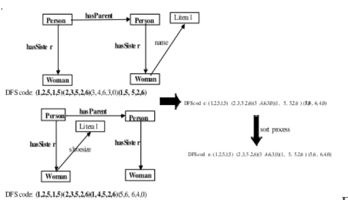
which node 5 (Person) is linked with another node 5 (Person) by the property 1 (hasParent). The edge (2,3,5,2,6) of the first DFS code does not have this link. So, the second discovery time of the edge (1,5,5,2,6) in the first DFS code is used to join the new edge. The edge (5,0,6,4,0) is added in the first DFS code to obtain an unsorted DFS code. A sort process allows to give discovery times with respect of Deep-First Search.

Figure 9 shows an example of such a join. Person hasParent hasSister Woman DFS code: (1,2,5,1,5)(1,3,5,2,6) Person Person hasParent name Litera l DFS code: (1,2,5,1,5)(2,3,5,3,0) DFS code: (1,2,5,1,5)( 1,3,5,2,6)(2,0,5,3,0) DFS code: (1,2,5,1,5) (2, 3,5,3,0) (1,4,5,2,6) sort process Person

In the two cases, after finding the discovery time m1 corresponding to m we set the discovery times of d1 at m1 and zero. Next, the edge d1 is added to the DFS code e2 after setting the kernel of each edge according to its presence in a DFS code. An ordering of DFS code e2 allows arranging the discovery time. After all graph patterns with n edges are generated from graph patterns with n-1 edges, if at least 2 of them are kept (they are non redundant and at least they have an instance in the repository) then the algorithm is recursively applied on the newly found graph patterns with n edges in order to generate graph patterns with n+1 edges and so on. The process stops when less than 2 graph patterns with n edges are generated and kept.

To improve the candidate evaluation we use an ask Sparql clause, as we are not interested by the frequency itself but only by the fact that at least one instance of the graph pattern exists in the dataset under consideration.

At last, note that we combine like [16] the growing and checking of subgraphs into one procedure, thus accelerating the mining process.

3. EXPERIMENTS AND PERFORMANCE

EVALUATION

Our algorithm is implemented in java and relies on the CORESE [2][4] semantic search engine for querying and reasoning on RDF datasets. CORESE implements the whole SPARQL syntax with some minor modifications (OPTIONAL is post processed, restriction on nesting OPTIONAL and UNION). It also implements RDF and RDFS entailments, datatypes, transitivity, symmetry and inverse property entailments from OWL Lite. The building of the index of an RDF repository is done after all these inferences have been done and the dataset has been enriched with the derivation they produced. More details on the formal semantics of the underlying graph models and projection operator are available in [1].

We tested our algorithm on a merge of three datasets: personData of DBPedia, a foaf dataset used by Edelweiss Team in course on semantic Web and a tag dataset of delicious. The resulting dataset contains 149882 triples and includes various graph patterns. The following table shows the result of our experiment. Each line summaries the results associated with the discovery of graph patterns of given size (shown in the first column). Column 2 shows the total number of graph patterns generated (GP) by our algorithm. Column 3 shows the number of graph patterns not kept (NKP) because redundant with other graph patterns of the same size. Column 4 shows the number of graph patterns generated but not kept (NFP) in the final index structure because having no instance in the dataset. Column 5 shows the number of graph

patterns removed from the index structure when generating graph patterns of size n+1 because included in graph patterns of size n+1 (DP). Finally, column 6 shows the number of DFS codes kept in the final index structure (KP). Column 7 shows the computation time in second (CP) and column 8 the number of join operation (JO).

Table 2: Result on merged dataset L e GP NKP NF P DP KP CP Jo 1 _{22 0 0 21 1 7,124 0} 2 _{72 0 9 63 0 0,228 57} 3 _{402 182 83 135 2 1,441 392} 4 _{642 343 42 250 7 0,953 641} 5 _{1128 672 12 428 16 1,663 1127} 6 _{1828 1152 5 639 32 1,889 1828} 7 _{2374 1519 1 798 56 1,61 2374} 8 _{2481 1563 0 845 73 1,58 2481} 9 _{2215 1377 0 755 83 1,67 2215} 10 _{1626 989 0 556 81 1,28 1626} 11 _{946 560 0 308 78 0,88 946} 12 _{408 232 0 119 57 0,33 408} 13 _{123 67 0 28 28 0,09 123} 14 _{23 12 0 3 8 0,02 23} 15 _{2 1 0 0 1 0 2}

In this example the algorithm finds a maximum graph pattern of size 15. The number of null frequencies is null from level 8. It means that we have a compact database from level 8 and all the candidate graph patterns are in the dataset. The percent of graph patterns marked to be deleted is 90,44%. The number of redundancies between join operation is high yet and one of our perspective is to reduce it.

Figure 10 shows the biggest RDF graph pattern generated.

4. CONCLUSION

In this paper we presented an algorithm to extract a compact representation of the content of an RDF triple store. This algorithm relies on DFS code based on canonical representation of graph patterns. We adapted this coding to deal with RDF graphs. We also provided a join operator to significantly reduce the number of generated graph patterns and we reduced the index size by keeping only the graph patterns with maximal coverage.

hasFather trousersize Person shirtsize age name shoesize Person shirtsize age name shoesize trousersize Person hasFriend name Person hasFriend name * * * * * * * * * * * *

Figure 10: The biggest graph pattern generated

Person hasParent hasSiste r Woman DFS code: (1,2,5,1,5)(2,3,5,2,6)(3, 4,6,3,0)(1,5, 5,2,6) Person Person has Parent

s hoesize

Litera l sort process Person hasSiste r Woman name Litera l hasSiste r Woman hasSiste r Woman DFS code: (1,2,5,1,5)(2,3,5,2,6)(1, 4,5,2,6)(5,6, 6,4,0) DFS c od e: ( 1,2,5,1,5) (2 ,3,5 ,2,6)(3 ,4,6,3,0)(1, 5, 5,2,6 ) (5,0 , 6, 4,0) DFS cod e: (1,2,5,1,5) (2 ,3,5 ,2,6)(3 ,4,6,3,0)(1, 5, 5,2,6 ) (5,6 , 6,4,0) F igure 9: Instance of joining two DFS codes of size 4.

Several perspectives of this contribution are already being considered. First, instead of using the sub-procedure timeEqual to compute exactly the discovery time corresponding to m we plan to add more redundancies and to test their frequencies to avoid the isomorphism test. Moreover, up to now, we do not take into account the RDFS schema the indexed dataset relies on. In our algorithm we only exploit the types of subject, object and properties of the triples. One of our main perspectives is to take into account the RDFS schema when building the index, at least by exploiting the subsumption relationship.

And in the long term, we also plan to provide means to support query decomposition with regards to index contents in the context of distributed datasets.

5. REFERENCES

[1] Baget, J-F., Corby, O., Dieng-Kuntz, R., Faron-Zucker, C.,

Gandon, F., Giboin, A., Gutierrez, A., Leclère, M., Mugnier, M-L., Thomopoulos, R.: Griwes: Generic Model and Preliminary Specifications for a Graph-Based Knowledge Representation Toolkit, ICCS , to appear in LNCS, (2008)

[2] Battle R., Benson E., Bridging the semantic Web and Web

2.0 with Representational State Transfer (REST), Web Semantics: Science, Services and Agents on the World Wide Web, Volume 6, 61-69, 2008.

[3] Corby O., Dieng-Kuntz R, Faron-Zucker, C.: Querying the

Semantic Web with the CORESE Search Engine. ECAI, IOS Press (2004)

[4] Corby, O.: Web, Graphs & Semantics, ICCS, to appear in

LNCS, (2008)

[5] Gandon F., Agents handling annotation distribution in a

corporate semantic Web, Web Intelligence and Agent Systems, IOS Press Internatio Journal, (Eds) Jiming Liu, Ning Zhong, Volume 1, Number 1, p 23-45, ISSN:1570-1263, 2003

[6] Gandon F., Lo M., Niang C., Un modèle d'index pour la

résolution distribuée de requêtes sur un nombre restreint de bases d'annotations RDF, 2007.

[7] Han J., Xie Z., 1994, Join index hierarchies for supporting

efficient navigations in object-oriented databases. In Proc. of the International Conference on Very Large Data Bases, pages 522–533, 1994.

[8] Han S., Keong Ng W., and Yang Yu, "FSP: Frequent

Substructure Pattern Mining ," In Proceedings of the 6th International Conference on Information, Communications and Signal Processing (ICICS'07) , Singapore, 10-13 December, 2007.

[9] J. Huan, W. Wang, and J. Prins. Efficient Mining of

Frequent Subgraphs in the Presence of Isomorphism. Proc. 3rd IEEE Int. Conf. on Data Mining (ICDM 2003, Melbourne, FL), 549–552. IEEE Press, Piscataway, NJ, USA 2003

[10] A. Inokuchi , T. Washio , H. Motoda, An Apriori-Based Algorithm for Mining Frequent Substructures from Graph Data, Proceedings of the 4th European Conference on Principles of Data Mining and Knowledge Discovery, p.13-23, September 13-16, 2000

[11] M. Kuramochi and G. Karypis. Frequent subgraph discovery. In Proc. 2001 Int. Conf. Data Mining (ICDM’01), pages 313–320, San Jose, CA, Nov. 2001.

[12] Maduko, A., Anyanwu, K., Sheth, A., Schliekelman, P., Graph Summaries for Subgraph Frequency Estimation, 5th European Semantic Web Conference (ESWC2008), Tenerife, June 2008.

[13] Prud'hommeaux E., Federated SPARQL, http://www.w3.org/2007/05/SPARQLfed/, 2004.

[14] Stuckenschmidt H., Vdovjak R., Jan Houben G., Broekstra J., Index structures and Algorithms for querying Distributed RDF Repositories, in Proc. WWW conference, 10-14, 2004.

[15] N. Vanetik, E. Gudes, and S. E. Shimony. Computing frequent graph patterns from semistructured data. In Proc. 2002 Int. Conf. on Data Mining (ICDM’02), pages 458–465, Maebashi, Japan, Dec. 2002.

[16] Yan X., Han J., gSpan: Graph-Based Substructure Pattern Mining, In ICDM 2002

[17] Yan X., Han J., CloseGraph: Mining closed frequent graph patterns, In Proc. 2003 Int. Conf Knowledge Discovery and Data Mining (KDD’03), Pages 286-295, Washington, D. C., Aug 2003.

[18] Yan X., Yu P. S, Han J., Graph Indexing: A Frequent Structure-based Approach, In SIGMOD, 2004.