A Multi-Physics PWR Model for the Load Following

HAL Id: hal-01355257

https://hal.archives-ouvertes.fr/hal-01355257

HAL is a multi-disciplinary open access archive for the deposit and dissemination of sci-entific research documents, whether they are pub-lished or not. The documents may come from teaching and research institutions in France or abroad, or from public or private research centers.

L’archive ouverte pluridisciplinaire HAL, est destinée au dépôt et à la diffusion de documents scientifiques de niveau recherche, publiés ou non, émanant des établissements d’enseignement et de recherche français ou étrangers, des laboratoires publics ou privés.

A Multi-Physics PWR Model for the Load Following

Mathieu Muniglia, Jean-Michel Do, Le Pallec Jean-Charles, Hubert Grard,

Sébastien Verel, S. David

To cite this version:

Mathieu Muniglia, Jean-Michel Do, Le Pallec Jean-Charles, Hubert Grard, Sébastien Verel, et al.. A Multi-Physics PWR Model for the Load Following. International Congress on Advances in Nuclear Power Plants (ICAPP), Apr 2016, San Francisco, United States. �hal-01355257�

A MULTI-PHYSICS PWR MODEL FOR THE LOAD FOLLOWING

Mathieu Munigliaa,*_{, Jean-Michel Do}a_{, Jean-Charles Le Pallec}a_{, Hubert Grard}b_{, Sébastien Verel}c_{, Sylvain David}d

a_{CEA/DEN/DM2S/SERMA, 91191 Gif-Sur-Yvette, France} b_{CEA/INSTN/UEINE , 91191 Gif-Sur-Yvette, France}

c_{Univ. Littoral Côte d’Opale, EA 4491 – LISIC – Lab. d'Informatique Signal et Image de la Côte d'Opale, Calais, France} d_{CNRS/IPNO , 15 Rue Georges Clemenceau, 91400 Orsay, France}

*_{mathieu.muniglia@cea.fr}

In this paper, a new model of a Pressurized Water Reactor (PWR) is described. This model includes the description of the core as well as a simplified secondary loop : the goal is to reproduce a load-following type transient, where the output power of the plant is controlled by the electric grid. Consequently, the control systems are also modeled, as the control rods or the soluble boron. The reference power plant is a 1300MW electrical PWR, managed with the french “G” mode. I. INTRODUCTION

In the actual context of energetic transition, the increase of the renewable energies contribution (as wind farms, solar energy, or biomass) is a major issue. Their intermittent production may lead to an important imbalance between consumption and production[1], and the others power plants must adapt to those variations, especially nuclear energy which is the most important in France. This paper is included in the study of the effects on the nuclear power plants (NPP) of a large introduction of renewable intermittent energies : how to optimize NPP toward a larger manageability, meeting the safety constraints. During an electrical power transient (demand of the grid) a chain of feedback is setting up in the whole reactor, leading to a new steady state. The reactor is designed to ensure that those feedback are stabilizing : we can take advantage of this self regulation in the case of small variations. Nevertheless, in the case of load following, the temperatures may be too different from the reference ones and may cause damages to the whole system. The control rods are used in order to manage with this variation, and maintain the primary coolant temperature close to the reference. The problem is that axial or radial heterogeneity of the neutron flux (and also of the thermal power and fuel temperatures) can occur, possibly leading to Xenon oscillations and/or to important power peaks. To try to improve the management, a multiobjective optimization approach is used, which minimizes the different values of interest (like the axial

offset or the power peak) : meta-heuristics methods[2] explore the possible configurations of velocity, overlap, etc, and their performances are computed by the model during a load-following transient. The computations are performed thanks to the APOLLO3®[3] code, using a whole reactor model including both neutronics, thermal-hydraulics and fuel thermal effects. Moreover, an operator model has been developed, to ensure a good management of the core, the main goal here being to reduce as much as possible the axial perturbations induced by the means of control.

The computation time is a major issue, and has to be as short as possible knowing that the optimization process will run thousands of calculations. Therefore we tried to simplified as much as possible the models. This paper is devoted to the multi-physics model, and the results of the simulation on a power transient are presented and compared to a model based on a NPP feedback. The latter is running a point kinetics neutronics calculation, which is not able to give information on the spatial perturbations.

II. SPECIFICATION OF THE CASE-STUDY II.A. Main Characteristics of the Core

The studied reactor is a 1300MW PWR (producing about 3800 thermal MW). The reactor core is a grid of square assemblies in a cylindrical vessel. Each assembly is 21cm side length and about 4m height. There are 193 assemblies, split into two kinds : 120 assemblies made of Uranium oxide (UOX) and 73 ones made of Uranium plus Gadolinium oxides (UGd). Fig. 1 shows the core of the reactor : the UOX assemblies are in orange and the UGd ones in purple. This figure also shows reflectors in green, standing for the iron vessel.

This reactor is managed with the GEMMES mode, which properties are :

• 18 month campaigns,

• a third core reloading,

• a maximal burn-up of 52 GWd/t,

• a 4% Uranium 235 enrichment,

• a AFA-3GL reference assembly.

Fig. 1. The different kinds of assemblies in the core, and their position (UOX in orange, UGd in purple).

The control rods are made of pins of a neutron absorber, and are inserted together from the top of the core in some assemblies. The positions of the assemblies where they are inserted are shown on Fig. 2. and correspond to the french “G” mode[4].

Fig. 2. Position of the assemblies where the control rods are inserted.

There are two kind of rods in the “G” mode :

• the black rods made of very absorbing pins (B4C

and Ag+In+Cd),

• the gray rods giving their name to the mode,

made of less absorbing pins (stainless steel and Ag+In+Cd).

Those rods are then split into two groups, depending on their function :

• the rods in charge of the power effects shimming

(PS) : 4 gray rods G1, 8 gray rods G2, 8 black rods N1, 8 black rods N2,

• the rods in charge of the regulation of the

primary coolant temperature (R) : 9 black rods R.

All the rods of a family (G1,G2,...) move together, and the families are inserted successively in this order, following an insertion program, in order to produce as less perturbations as possible. The position of the thimble tubes where are inserted the pins are shown on Fig. 3.

Fig. 3. Position of the pins inside the assembly, for a gray rod (left) or a black one (right). The fuel pins are in

yellow, the stainless steel pins in gray and the B4C+AIC

pins in black.

II.B. Regulated variables

The electrical power variations from the grid result in variations of the turbine rotation speed, leading to a whole series of repercussions on the core, and it is not acceptable, in case of the load-following, to let the core evolve. Indeed, the temperature and pressure conditions may be too different from the nominal conditions. Before we define the controlling chains in charge of this regulation, we focus on the regulated variables, and their set value in function of the power. We will not propose an exhaustive list, but the minimal one, necessary to the understanding of the problem.

It is known that the primary coolant temperature and the secondary pressure are strongly coupled through the steam generator. There are two point of view : (1) the primary coolant temperature is kept constant, which minimizes the neutronics effects to be offset, but maximizes the pressure variations leading to an over-sizing of the secondary's components; (2) the pressure is

kept constant, which maximizes the control rods movement. A compromise has been defined and neither the secondary pressure nor the primary coolant temperature is constant, but they are function of the power. The temperature program is plotted on Fig. 4 as a function of the thermal power (in percent of the nominal power).

Fig. 4. Primary coolant temperature program for a PWR 1300MW.

The control rods and the soluble boron will then be used to maintain the average coolant temperature as close as possible to the reference one, and the secondary pressure is a free variable. The values of the temperatures at nominal or at zero power come also from compromises, between efficiency and safety. We will not enter into details here, for more details one can refer to [5].

We can also mention other processed values as (see [6] for more details) :

• the primary pressure, must be sufficient to avoid

boiling at 325°C, but still lower than the limit pressure corresponding to the pipes breaking point (set value is 155 bar in our case),

• the water level in the pressurizer (which changes

during the primary pressure regulation) enabling to keep the pressurizer in safe conditions, and to keep constant the primary coolant mass,

• the water level in the steam generators (function

of the power) controlling the efficiency of the heat transfers between the primary and the secondary circuits.

II.C. Control systems

There is at least one control system for each regulated value : one for the primary pressure, one for the water level in the pressurizer and in the steam generators, one for the turbine rotation speed, one for the turbine by-pass, and one for the primary coolant temperature. We will describe only the latter, assuming that the others work

exactly as they should, and that the values they control stick to their set point.

The control of the primary coolant temperature is composed of two parts : the control rods and the soluble boron concentration. The main difference is that the first one is fully automated, whereas the second one is controlled by the operator.

II.C.1. Control rods

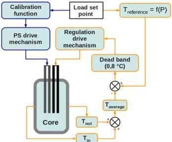
The moderator and the Doppler effect are stabilizing : if a rise of the temperatures occurs, these effects cause a reduction of the reactivity, leading to a decrease of the power, and of the temperatures. This is the case if the demand of the grid decreases : the steam flow is reduced, the heat exchanges in the steam generator are less efficient and the primary coolant temperature increases. To anticipate the process, the position of the power shimming rods is directly function of the electrical power : the thermal power is reduced and the important variations of the temperature are avoided. To do so, a calibration function is established at the beginning of the cycle, giving the position of the rods as a function of the power. This curve is updated every 60 equivalent full power days (EFPD), in order to take into account the burn-up effects. Still, between the last update and the next one, slight discrepancies occur, and the temperature is adjusted thanks to the temperature regulation rods. The former is then managed in open loop (blue), and the latter in closed loop with a feedback (orange), as we can see on Fig. 5.

Fig. 5. Control rods drive mechanisms. The PS drive mechanism is in open loop whereas the temperature regulation is in closed loop.

A dead band of 0.8°C has been implemented to avoid continuous displacement of the regulation rods. The

average core temperature is compared to the reference one, and if the absolute difference is within this dead band, the core is self-regulating.

The speed of the power shimming rods is 60 steps per minute (one step is about 1.65 cm, and the core is 260

steps height). The regulation rods have a maximal (vmax =

72 steps/min) and a minimal (vmin = 8 steps/min) speed,

and the real one depends on the difference of the previous temperatures :

• 0 steps/min if |Tref – Tm| < 0,8

• vmin if 0,8 < |Tref – Tm| < 1,7

• linear between vmin and vmax if

1,7 < |Tref – Tm| < 2,8

• vmax if Tref – Tm| > 2,8

This speed program is plotted on Fig. 6.

Fig. 6. Regulation rods speed program. The speed is positive in case of removal and negative during insertion.

Even if the power shimming rods are able to move on the whole height of the core, the regulation rods are shut within a maneuvering band which height is 27 steps in the upper part of the core. This should enable to keep a negative reactivity margin, and to avoid under-depletion of the assemblies in which they are inserted.

II.C.2. Soluble Boron

It enables to control the reactivity when the variations are slow, or if the control rods are no longer able to do it (regulation rods at the edge of their maneuvering band). It is used for instance to offset the burn-up effects, or the xenon effects after important load variations.

Fig. 7 represents a simplified diagram of the mechanism in charge of the boron concentration regulation in the primary circuit.

Fig. 7. Simplified soluble boron management diagram. The primary fluid is collected from the cold leg, then cooled through a heat exchanger and expanded. The temperature and pressure conditions must be compatible with the demineralizers (not on the diagram). After the demineralizers, the fluid is either gathered in the volume control tank or in the boron recycling to be treated.

Then if a boration is needed, this fluid is mixed with the boric acid coming from the boron injection tank and is re-injected in the primary loop. The injected boron concentration is then 7700 ppm. If a dilution is needed, the injected fluid is demineralized water (0 ppm). The fluid is preheated by the collected fluid before it is re-injected. We will consider in our case a maximal charging flow rate of :

• 30 t/h in the case of dilution

• 10 t/h in the case of boration

To sum up, the power shimming (PS) rods compensate the main effects of a power variation, but as their regulation is in open loop, their is some adjustment to do with the regulation (R) rods. The boron compensates the effects of the poisons as well as the slow decrease of the core reactivity (burn-up effects).

It is used also to avoid large variations of the Axial Offset (AO). For example, if the AO is too large (high power in the half top of the core), the operator reduces the boron concentration (dilution) to increase the temperature. Automatically, the regulation rods will insert and consequently reduce the power in this half top.

III. DESIGN OF THE CALCULATION MODEL III.A. Model of the primary loop

The primary loop is composed of several important systems. The main are : the core, the steam generators, the pressurizer and the primary pumps. We will consider in this study only the core and the steam generators : all the other ones are considered perfect. The pressurizer keeps constant the primary pressure to 155 bar, and the primary pumps are always in service. The steam generators will be described in the next section, dedicated to the secondary

circuit. The following describes the adopted models, parts of the multi-physics calculation of the core.

III.A.1. Neutronics

The neutronics part of the calculation consists in a quasi-static model, in which spatial and time aspects are decorrelated. The spatial effects are determined with a 3D diffusion calculation, and the time is taken into account through a point kinetics. The geometry is a quarter of core (with reflection boundary conditions to reconstruct the whole core, and void conditions along the vessel), with four slabs per assembly, and 34 axial meshes. Each

calculation mesh is then a 10.7∗10.7∗14.2 cm3 _{cube, and}

we have 9826 of them in the quarter of core.

Knowing the boundary conditions (inlet temperature and enthalpy) a first 3D calculation is performed, in order to determine the reactivity. The power is then updated thanks to the linearization of the Nordheim's formula in case of small reactivities. In a third step, the shapes of the power and temperature are calculated in a second 3D calculation. Here after, the equations describing the 3D diffusion calculation as well as the point kinetics.

The diffusion equation is derived from the general Boltzmann equation, assuming some hypothesis :

• phase flux dependence on angle is small

• there is little heterogeneity, so that not much

information is lost during homogenization of the media

• one is far from the interfaces

• the absorption macroscopic cross section is small

compared to the diffusion one, that is to say the neutrons undergo a lot of collisions

• the variations in space and time of the considered

variables are small

After these simplifications of the transport equation, one get the diffusion equation for the group g :

⃗ ∇ [Dg(⃗r ) ⃗∇ ϕg(⃗r )]−Σagϕg(⃗r )+

∑

∑

∑

ϕ is the scalar flux,

D is the diffusion coefficient,

Σ are the macroscopic cross sections,

χ is the energy spectrum (proportion of neutrons

emitted in the group g per fission),

ν is the number of fission neutrons.

The subscripts correspond to the group, and the superscripts to the type of reaction : a stands for absorption, s for scattering, and f for fission.

We assume a two group calculation, and the mixed dual finite elements method[7] of the APOLLO3 code is used.

Concerning the point kinetics, the coupled equations written in terms of neutrons population and precursors concentration are :

{

∑

n is the total number of neutrons,

Ci the concentration of the precursors in the

family i,

ρ the reactivity,

keff the effective multiplication factor,

l the mean neutrons lifetime in the reactor,

β_i the number of delayed neutrons from the

family i of precursors,

β its average over all the families,

λ_i the decay constant of the family i.

The solution of this system (2) is a linear

combination of I+1 particular solutions, where I is the

number of families. Those particular solutions are considered to be exponential. Thus, the general solutions

can be wrote n(t)=∑j Ajexp(ωjt ). It can be shown that

the ω_j (j=0,1, ...,I ) are solutions of the following

equation called Nordheim equation :

ρ= l keff ω+

∑

In our case, we assume a small reactivity : equation (3) can be linearized, and the expression of the largest root become simply :

ω₀≃ρ_τ (4) with τ= l keff +

∑

∑

τ represents a time, characteristic of the fissile

nucleus. We took τ=0,06 s. Finally, the neutron

population evolves as : n(t)=n0exp(

ρ

as well as the total power of the core.

The poisons like Xenon, Iodine or Samarium are also calculated with the 3D node, using simplified decay chains, and their concentrations are updated every time step.

III.A.2. Primary Thermal-Hydraulics

The thermal-hydraulics calculation of the primary circuit is simply an enthalpy balance between the bottom and the top of each mesh, knowing the power per calculation mesh (the geometry is the same as previously). In the following equation, the fluid temperature is supposed constant radially, and the fluid temperature and density are related to the enthalpy by the state equations of the fluid. Moreover, a steady state is determined, considering that the variations of the fluid properties are slow, e.g. constant during a time step :

dH (z)

dz =

πDtΦ

S_hv ρ( H ) (7)

with

H the enthalpy (in J /g),

Dt the sum of the diameters of the pins in the

mesh (in cm),

Φ the heat flux between the pins and the fluid (in

W / cm2_),

Sh the hydraulic section (in cm

2 ),

v the average fluid velocity (in cm/ s),

ρ the fluid density (in g/cm3_).

III.A.3. Fuel Thermics

This part of the calculation gives more information on the temperatures inside the fuel pellet: the evolution of the fluid temperature changes the boundary conditions of the cladding and modifies the temperature profiles (and the average temperature) inside the pellet. The following heat equation is written assuming a constant temperature over the height of the mesh, and a uniform power production inside the mesh. Here again, we deal with the stationary problem assuming slow variations of the temperature and power.

−1 r d dr(r λ (T ) dT (r ) dr )=Pvol (8) where

λ is the thermal conductivity (in W / cm/ K),

T the temperature (in K),

Pvol the power density (in W / cm

3 ).

The conductivity is defined as a series of polynomial functions, in different ranges of temperature.

III.B. Model of the Secondary System III.B.1. Components of the Secondary System

The secondary circuit is the part of the power plant in charge of the electrical production. The main components of this loop are then : the steam generators, the turbine, the alternator, the condenser, and several pumps. Obviously, they are a lot of other components, but we will not enter the details.

The turbine, the alternator and the condenser are supposed perfect :

• the turbine and the alternator are simply

replaced by the theoretical electrical power required by the grid

• the condenser provides a constant inlet

temperature to the steam generators.

But in order to take into account the effects of an electrical power variation, we need a model of the steam generators. This will enable to reproduce the delay between variations in the secondary circuit and the ones in the primary circuit.

In order to be a bit more realistic, we also consider the variation of the efficiency as a function of the power. Indeed, the conversion from thermal power to electrical power is better when the temperatures are important, that is to say when the power is high.

III.B.2. Steam Generator

As the phenomena occurring in the four loops are supposed to be identical, only one of them is considered. The model simulates a natural circulation U-tube steam generator, and the idea is to determine the transferred

power (PSG). This power depends on the average

temperature of the primary fluid, given by the thermal-hydraulics calculation presented before :

PSG=HS(Tm−Tsat) (9)

with

Hs a coefficient corresponding to the surface of

the tubes over the thermal resistance (in W / K),

Tm the average temperature of the primary fluid

(in K),

Tsat the saturation temperature of the secondary

fluid inside the steam generator (in K).

Thus, this power variation gives the variation of the inlet temperature of the core :

ΔTi n=− 1_mC p

with

m the total mass of the primary circuit (kg),

Cp the heat capacity (J/kg/K),

dt the time step.

The saturation temperature in Eq. (9) depends on the density of the secondary fluid in the steam generator, itself depending on the balance between the production and the evacuation of the steam. Those flow rates are respectively linear functions of the steam generator power and of the electrical power. At nominal power, they are the same.

III.C. Calculation Scheme

Each model described previously corresponds to a box in the Fig. 10, and we discuss in this part the way they are organized and the different time steps.

Fig. 8. Calculation scheme.

First, it is obvious that in a core all those elements occur at the same time. For numerical and calculation time reasons, we decided to treat them one after another, implying some hypothesis. The position of the power shimming rods is automatically modified knowing the electrical power and the calibration function. This induces

a modification of the average temperature of the core, which, combined to the modification of the conditions in the steam generator otherwise, leads to a new state of the primary fluid. The poisons effects are took into account before the adjustment of the temperature and axial offset, as it is done in operation.

The choice of the time steps is of primary importance is the calculation scheme. The step time corresponding to the coupling between the primary and the secondary

circuit (dt2) must be short enough to consider mCp in Eq.

(10) as a constant, but not too much to limit the computation time. The value of the time step

corresponding to the power variations (dt1) results also

from a compromise : if it is too long, the power variation leads to a move of the control rods during a too long time, incoherent with the sequential point of view. To the contrary, if it is too short, the number of coupling iterations is not sufficient to reach a representative state (dt1=''number of loops''⋅dt2, ). dt3 is equal to dt1 because the time is not incremented in this loop : as long as the boron concentration is not satisfactory, the neutronics calculation is canceled and the previous state is restored.

IV. RESULTS AND ANALYSIS IV.A. Calibration Function

The calibration function we obtained is shown on Fig. 9. Each relative power corresponds to a number of inserted steps (power shimming). To determine these points, we calculate a series of static steps, at the different power, performing a research of the critical rods position. The idea of this calibration is to avoid all the other sources of reactivity, so the regulation rods stay at the same place (middle of their maneuvering band) and the poisons remain constant (concentrations equal to the ones determined at nominal power). One can see also on this curves the burn-up effect : the effects to compensate increases as the burn-up increases. Consequently, the power shimming rods are under-inserted almost all the time, and the remaining is done by the regulation rods or the soluble boron.

IV.B. Numerical Simulation of the PWR on a Power Transient

IV.B.1. The Load-following scenario

The transient corresponds to a typical load-following, with ramps at 5%PN/min (percent of nominal power per minute), and two plateau at 30% and 100% of the nominal power. It is shown on Fig. 10.

Fig. 10. Evolution of the electrical and reference thermal power. The calculated thermal power is also plotted.

The first thing to notice is the difference between the electrical and the reference thermal power : the efficiency is not constant and depends on the electrical power. Moreover, one can see the inertia of the system, evolving a little bit like a second order system (fast response and overshoot). The following results have been obtained with

the step times such as dt1=dt3=90s and dt2=15s.

IV.B.2. Evolution of the power plant

The following figures present the evolution of the main values of the power plant, like the temperatures, the boron concentration, and the rods position. Several models are compared, to see their influence on the evolution. More precisely, the label “no operator” means that the transient have been done with the idea of modifying the boron concentration only if necessary e.g. only if the difference between the average temperature

and the reference is greater than 0,8 °C. The label “no ΔI

max” (ΔI= AO⋅''relative power'') corresponds to a model

in which a very simple operator adjusts the average

temperature in a ±0,2° C band thanks to the boron. The

two previous models do not integrate the regulation on the Axial Offset. The last and the most completed model simulates the actions of a more realistic operator. To do so, the regulation rods position and the boron concentration are tuned jointly, to ensure both a satisfactory temperature and axial offset. Fig. 11, 12 and 13 show respectively the evolution of the boron and

Xenon concentrations, of the regulation rods position and of the average temperature in the core.

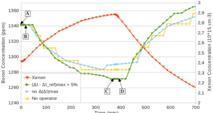
Fig. 11. Boron and Xenon concentrations during the transient.

In the simplest model (yellow), the boron concentration is a piecewise constant function: the concentration is adjusted periodically. By introducing a

fictive dead band of 0,2 ° C, this yellow curve is smoothed

and one gets the blue curve. If we control the Axial Offset, the amplitude is greater (green) meaning that the use of boron increases. For example, on the lower plateau, the axial offset of xenon concentration makes the axial offset of power increases. The operator dilutes the boron, to automatically insert the regulation rods (rise of the temperature), decreasing the axial offset. The opposite is happening on the upper plateau. This can be seen also on the Fig. 12, where the inserted steps increases (resp. decreases) at the same time. An interesting thing to observe on Fig. 12 is that the regulation rods tend to come back to their initial position. The axial offset set point (Fig. 14) is indeed determined at nominal power, with homogeneous xenon concentration, and regulation rods at the middle of their maneuvering band. To see whether the management is efficient or not, one plots in Fig. 14 the

current point of the core in the (ΔI , Pr) plane, called the

control diagram.

Fig. 12. Position of the regulation rods during the transient.

Fig. 13. Average temperature during the transient.

This Fig. 14 shows the main effects of the axial offset control. To show their influence on the upper plateau also, we have continued the transient until 18h. Indeed the observed drift occurring on the lower plateau also takes place at the end of the transient, and has to be handled as well.

Fig. 14. Control diagram, showing also the limits.

In case of no control, the AO over-goes the limits which are defined as regard to safety (red line). This is obviously unacceptable, and avoided with the control. The axial offset is kept in a reasonable range and a safe behavior of the core is ensured : the power and flux profiles are more and more flat, and the risks due to high power peak decrease. However, a xenon oscillation is still not prevented.

The current state of the poisonous fission products is unknown, and it could be such as a xenon oscillation is setting up. The Shimazu[8] diagram here after brought further information about the state of the reactor after the transient, linking together the axial offset of xenon (AOx), iodine (AOi) and power (AOp). The transient was continued until 72 h this time.

Fig. 15. Shimazu diagram.

An ellipse show up, characterizing the oscillation. If it converges the oscillation is stable, meaning that the core is getting into a stable state, corresponding to the center of the ellipse. This is the case in the two models presented here.

IV.B.3. Benchmark with other models

The consistency of the results have been discussed, and we know compare them with another model[2]. This is a point kinetics model for the neutronics, but propose a more refined description of the secondary system, and is based on a power plant and simulator feedback. Thus, even if it is not a best-estimate model, the goal here is to ensure a behavior close to the reality.

This model is called “0D Model” in the following, and the model we have developed is called “3D Model”. The comparisons between the two models are presented for several variables as the thermal power (Fig. 16), the boron concentration (Fig. 17) and the average temperature of the coolant (Fig. 18).

The thermal power is expressed in percent of the nominal power.

Fig. 16. Comparison of the thermal powers obtained with the two models.

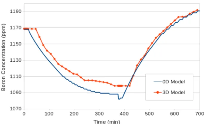
Fig. 17. Comparison of the boron concentrations.

To compare the evolution of the boron concentration, we have shifted the results of the “3D Model” to fit the blue curve. The difference between the initial values (about 170 ppm) is due to a different burn-up between the two models : we have considered a core at the beginning of the cycle, whereas the “0D Model” starts from 10% of the cycle, thus starting from a lower boron concentration.

Fig. 18. Comparison of the average coolant temperatures. The results match very well the “0D Model” showing that the general behalf of the core is well reproduced.

Concerning the calculation time, the transient corresponding to 700 minutes (almost 12 hours) has been realized in 25 minutes on a personal computer (Intel®

Xeon® @2,1 GHz). Here again it is very promising and

we can do even better by releasing the convergence criteria of the neutronics calculation for example.

V. CONCLUSIONS

A model of a PWP has been presented, and the results has been discussed and compared to another model based on a simulator feedback. The goal of this new model is to give physical information on the core during a power transient and for different management of the control rods and soluble boron. It will then be possible to choose,

among all the possibilities, the ones enabling a faster response of the core, while keeping it safe.

From this point of view this model meets the expectations, as it reproduces well the behavior of the nuclear power plant, and can give global values (average on the whole core) as well as local ones (per calculation mesh). Further developments are devoted to find the best compromise between precision and computation time.

ACKNOWLEDGMENTS

The authors would like to thanks IDEX and PS2E for their financial support. We gratefully acknowledge AREVA and EDF for their long term partnership and support.

REFERENCES

1. Bilan prévisionnel de l’équilibre offre-demande d’électricité en France, RTE (2014).

2. T. El-Ghazali, Meta-heuristics, from design to

implementation, John Wiley & sons (2009)

3. H. GOLFIER et al., “APOLLO3 : a common project of CEA, AREVA and EDF for the development of a new deterministic multi-purpose code for core physics analysis,” M&C, Saratoga Springs, New York, May 3-7 2009.

4. A. Lokhov, “Technical and economic aspect of load following with nuclear power plants”, Nuclear Energy Agency, OECD, June 2011.

5. H. GRARD, Physique, fonctionnement et sûreté des

REP, EDP Sciences (2014).

6. P. COPPOLANI et al., La chaudière des réacteurs à

eau sous pression, EDP Sciences (2004).

7. J.-J. LAUTARD, F. MOREAU, “A fast 3D parallel solver based on the mixed dual finite element approximation,” Proceedings ANS Topical Meeting, Mathematical Methods and Super-computing in Nuclear Applications, Karlsruhe, Germany, April, 1993.

8. Y. SHIMAZU, “Xenon Oscillation Control in Large PWRs Using a Characteristic Ellipse Trajectory Drawn by Three Axial Offsets ,” Journal of NUCLEAR SCIENCE