HAL Id: hal-01584120
https://hal.archives-ouvertes.fr/hal-01584120
Submitted on 17 Sep 2020
HAL is a multi-disciplinary open access
archive for the deposit and dissemination of
sci-entific research documents, whether they are
pub-lished or not. The documents may come from
teaching and research institutions in France or
abroad, or from public or private research centers.
L’archive ouverte pluridisciplinaire HAL, est
destinée au dépôt et à la diffusion de documents
scientifiques de niveau recherche, publiés ou non,
émanant des établissements d’enseignement et de
recherche français ou étrangers, des laboratoires
publics ou privés.
recent large increases been detected?
M. Bruhwiler, S. Basu, P. Bergamaschi, P. Bousquet, E. Dlugokencky, S.
Houweling, M. Ishizawa, S. Kim, R. Locatelli, S. Maksyutov, et al.
To cite this version:
M. Bruhwiler, S. Basu, P. Bergamaschi, P. Bousquet, E. Dlugokencky, et al.. U.S. CH4 emissions from
oil and gas production: Have recent large increases been detected?. Journal of Geophysical Research:
Atmospheres, American Geophysical Union, 2017, 122 (7), pp.4070 - 4083. �10.1002/2016JD026157�.
�hal-01584120�
U.S. CH
4emissions from oil and gas production:
Have recent large increases been detected?
L. M. Bruhwiler1 , S. Basu2, P. Bergamaschi3, P. Bousquet4 , E. Dlugokencky1 ,
S. Houweling5,6 , M. Ishizawa7 , H.-S. Kim7, R. Locatelli4 , S. Maksyutov7 , S. Montzka1 , S. Pandey5,6, P. K. Patra8, G. Petron2 , M. Saunois4 , C. Sweeney2 , S. Schwietzke2 , P. Tans1 , and E. C. Weatherhead2
1
NOAA Earth System Research Laboratory, Boulder, Colorado, USA,2Cooperative Institute for Research in Environmental Sciences, University of Colorado Boulder, Boulder, Colorado, USA,3European Commission, Joint Research Centre, Ispra, Italy, 4
Laboratoire des Sciences du Climat et de l’Environnement, CEA-CNRS-UVSQ, IPSL, Gif sur Yvette, France,5SRON Netherlands Institute for Space Research, Utrecht, Netherlands,6Institute for Marine and Atmospheric Research Utrecht,
Utrecht, Netherlands,7National Institute for Environmental Studies, Tsukuba, Japan,8Japan Agency for Marine-Earth Science and Technology, Yokohama, Japan
Abstract
Recent studies have proposed significant increases in CH4emissions possibly from oil and gas(O&G) production, especially for the U.S. where O&G production has reached historically high levels over the past decade. In this study, we show that an ensemble of time-dependent atmospheric inversions constrained by calibrated atmospheric observations of surface CH4mole fraction, with some including space-based retrievals of column average CH4mole fractions, suggests that North American CH4emissions have beenflat over years spanning 2000 through 2012. Estimates of emission trends using zonal gradients of column average CH4calculated relative to an upstream background are not easy to make due to atmospheric
variability, relative insensitivity of column average CH4to surface emissions at regional scales, and fast zonal
synoptic transport. In addition, any trends in continental enhancements of column average CH4are sensitive to how the upstream background is chosen, and model simulations imply that short-term (4 years or less) trends in column average CH4horizontal gradients of up to 1.5 ppb/yr can occur just from interannual
transport variability acting on a strong latitudinal CH4gradient. Finally, trends in spatial gradients calculated
from space-based column average CH4can be significantly biased (>2–3 ppb/yr) due to the nonuniform and
seasonally varying temporal coverage of satellite retrievals.
Plain Language Summary
In this paper we address recent claims of significant increases in methane emissions from U.S. oil and gas production. Wefind that such claims are inconsistent with observations by examining atmospheric inversions and observations from the NOAA aircraft monitoring program. Furthermore, we show how atmospheric variability, sampling biases, and choice of upwind background can lead to spurious trends in atmospheric column average methane when using both in situ and space-based retrievals.1. Introduction
The global methane budget has received much attention in recent years [e.g., Kirschke et al., 2013; Nisbet et al., 2014, 2016; Schaefer et al., 2016], and to date, syntheses of regional methane budgets exist for South Asia [Patra et al., 2013], the Arctic [AMAP Assessment, 2015], North America [Miller et al., 2013], Europe [Bergamaschi et al., 2015] and South America [Wilson et al., 2016]. North America is thought to contribute 5–10% of global methane emissions [Kirschke et al., 2013]. The global CarbonTracker-CH4inversion estimates
that North American CH4emission account for 10% of the global total over 2000 to 2010 [Bruhwiler et al.,
2014]. A recent regional inversion study by Miller et al. [2013] found that annual U.S. CH4emissions are under-estimated by a factor 1.5 to 1.7 relative to inventories. Using Greenhouse Gases Observing Satellite (GOSAT) retrievals of satellite column average CH4for 2010–2014, Turner et al. [2016] reported a recent large increase in U.S. CH4emissions, about 20% per year relative to the Environmental Protection Agency (EPA) Greenhouse
Gas Inventory (GHGI) [US Environmental Protection Agency (EPA), 2016]. By considering surface observations, the results of three different atmospheric inversions and GOSAT retrievals, Turner et al. [2016] estimated that North American CH4emissions have risen by over 30% over 2002–2014. Such an increase would account for
30–60% of the global increase in atmospheric CH4observed since 2007 by NOAA’s Cooperative Air Sampling
Journal of Geophysical Research: Atmospheres
RESEARCH ARTICLE
10.1002/2016JD026157
Key Points:
• Atmospheric inversions using in situ observations do not support large increases in CH4emissions from U.S.
oil and gas production
• Short-term trends in spatial gradients of CH4column abundance are not
sensitive to changes in emissions due to atmospheric variability
• Temporal sampling gaps in satellite retrievals and choices of background can give spurious trends in column average CH4gradients
Correspondence to:
L. M. Bruhwiler, [email protected]
Citation:
Bruhwiler, L. M., et al. (2017), U.S. CH4
emissions from oil and gas production: Have recent large increases been detected?, J. Geophys. Res. Atmos., 122, 4070–4083, doi:10.1002/2016JD026157. Received 27 OCT 2016
Accepted 5 MAR 2017
Accepted article online 8 MAR 2017 Published online 7 APRIL 2017
©2017. American Geophysical Union. All Rights Reserved.
Network [Dlugokencky et al., 2011]. Turner et al. [2016] point out that they are unable to attribute the emission changes to individual sectors (e.g., livestock, agriculture, and fossil fuel production) but they suggest that O&G (oil and gas) production is likely to be behind the large increase they infer. Franco et al. [2016] proposed that U.S. O&G emissions increased by 15 TgCH4/yr over 2008–2014 based on ground-based Fourier transform
infrared (FTIR) observations of C2H6and a single C2H6/CH4emission ratio for U.S. O&G emissions. Hausmann
et al. [2016] also proposed large increases in CH4emissions based on their retrieval of column averaged CH4
and C2H6using a surface-based FTIR spectrometer at Zugspitze, Germany. They found that increases in fugi-tive emissions from O&G production (not necessarily attributable to the U.S.) account for 13–53% of the renewed global CH4growth since 2007. Helmig et al. [2016] pointed out that observed increases in ethane and propane could suggest large increases in U.S. CH4emissions from O&G production, but that such a
con-clusion would be inconsistent with other evidence, such as global observations of the methane isotope, δ13CH
4. Although observational evidence is compelling that atmospheric C2H6 has indeed increased, it is
rather more difficult to obtain the corresponding increases in CH4emissions because the ratio of methane to ethane emitted as a result of fugitive fossil fuel emissions is highly variable. Peischl et al. [2015, 2016] showed that this ratio could vary over 2 orders of magnitude based on measurements from four different U.S. O&G production regions.
Globalδ13CH4observations constrain the global contribution of microbial sources relative to nonmicrobial sources, such as fossil fuel production. Schaefer et al. [2016] showed that the observed trend in atmospheric δ13C toward more depleted values after 2006 puts an upper limit on the increase of thermogenic sources
(including fossil fuel emissions). They estimated that thermogenic emissions account for only 0.9 ± 4.8 TgCH4/yr of the recent global increase of 19.7 TgCH4/yr since 2006. The results of Nisbet et al. [2016] show a similar trend in atmosphericδ13C, and they suggest that increases in emissions from tropical wetlands, rice paddies, and ruminants are likely to be behind the recent global CH4increase. A recent study
by Schwietzke et al. [2016] makes use of a large set of globalδ13CH4observations to show that, while fossil fuel
and geologic emissions make up a larger share of global emissions than previously thought (60–110% greater), they have remained relatively stable over the past few decades even as production has increased. The question of whether CH4emissions from the U.S. O&G sector have increased is of importance, especially considering the potential spread of new extraction technologies developed in the U.S. to exploit unconven-tional O&G reserves. Natural gas is regarded by some as a potential“bridge” fuel until large-scale zero carbon energy becomes economically feasible, since its CO2emissions are half those from coal per unit of power
generated [Alvarez et al., 2012; Zavala-Araiza et al., 2015]. Coal production is also a source of atmospheric CH4[US Energy Information Administration (EIA), 2016]. However, supply chain leak rates must be small for
there to be a climate benefit from switching from coal to natural gas.
2. Inferring Emission Trends From Atmospheric Inverse Models
Atmospheric inversions combine atmospheric mole fraction observations, emissions from inventories and process-based models (“priors”), and atmospheric chemistry-transport models to infer spatially and tempo-rally resolved optimized (“posterior”) methane emissions and their uncertainties. The Global Carbon Project gathered 30 different global inversions provided by 8 different research groups worldwide for 2000–2012 (Saunois et al. [2016], updating Kirschke et al. [2013]). The different inversions (see Table 1) vary in the obser-vations assimilated (e.g., surface obserobser-vations and/or retrievals of column average CH4 from GOSAT or Scanning Imaging Absorption Spectrometer for Atmospheric Chartography, on Envisat (SCIAMACHY) space-borne instruments), the atmospheric chemical transport model used, and the inversion set up (prior emis-sions, prior uncertainties, and inverse technique). Assumptions made about uncertainty of the simulated observations due to transport errors and the uncertainties of prior emissions are particularly important because the relative size of these errors determines the weighting of observations relative to prior emissions in determining the solution. Optimized annual emissions for the U.S. have been extracted from this ensemble of inversion for 2000 to 2014 (Figure 1). In the following text, we will refer to inversions that sequentially esti-mate over time as“time dependent,” the alternative being estimation of time-averaged fluxes.
Figure 1a reveals that mean posterior emissions for the contiguous U.S. from the inversion ensemble show a large spread, varying from 30 to 50 TgCH4/yr on average over 2000–2012. The inversion
[e.g., Bousquet et al., 2006] have pointed out that interannual changes in emissions estimated by inverse modeling are more robust than long-term mean emissions, and the inversion ensemble shows a smaller spread among emission anomalies (Figure 1b). Inversions constrained by both surface observations and space-based retrievals of column average CH4also do not appear to yield noticeably different emission
estimates from those using only surface observations.
Ideally, to estimate a trend over a period fromflux inversions one should use a consistent inversion frame-work over the entire period. If different inversion methods are used for different parts of the period, the meth-ods should be comparable. However, that is not the case for the emission trend derived by Turner et al. [2016]. That emission trend (also shown in Figure 1) is based on estimates of U.S. CH4emissions from three different inversion systems: Wecht et al. [2014], Miller et al. [2013], and Turner et al. [2015]. As summarized in Table 1, these inversions differ significantly in estimation technique, observational constraints, temporal resolution, atmospheric transport model, boundary conditions, and prior emissions. A major source of difference among inversions is atmospheric transport, and Locatelli et al. [2015] showed that differences in modeled transport can change the source apportionment among regions. Although Wecht et al. [2014] and Turner et al. [2015] use the same atmospheric transport model, the regional approach of Miller et al. [2013] is very different and uses offline wind fields from a regional weather prediction model to drive a Lagrangian particle disper-sion model. Obtaining trend information from such different approaches requires that the methods be com-parable. Alternatively, a consistentflux estimation framework applied over the entire period could be used. A second important source of variation among inversions has to do with the choice of observations. Satellite column retrievals cannot be calibrated against World Meteorological Organization-traceable CH4standards and may have biases that vary spatially and over time [Monteil et al., 2013]. Even though GOSAT and SCIAMACHY are both shortwave infrared (SWIR) instruments, it has to be demonstrated that their retrievals are comparable enough to be used together for trend detection as done by Turner et al. [2016]. Miller et al. [2013] used observations from surface sites, aircraft, and towers (Table 1), and these in situ observations pro-vide specific information about CH4near the surface as well as its vertical distribution (rather than a column
average). Lack of data coverage, whether in situ observations or retrievals from space-based instruments, can lead to two problems: a solution that stays close to the prior estimate in unconstrained regions and an exag-gerated sensitivity to local sources. Bruhwiler et al. [2014] noted the influence of observations at Southern Great Plains (SGP), a site located near a rapidly expanding O&G basin in Oklahoma, on estimated CH4
emis-sions from North American O&G production. Increased CH4abundance over time at SGP may reflect a local
increase in regional emissions, but such a trend is not necessarily linked to national-scale emission changes. In the case of atmosphericflux inversions, the year-to-year variability of estimated emissions may reflect actual variability in sources, for example, the response of natural wetland emissions to temperature and precipitation, or it may be due to noise in the atmospheric inversion arising from misattribution of signals
Table 1. Characteristics of Inversions Used by Turner et al. [2016] Inversion Atmospheric Transport Model Observational Constraints Time Prior Emissions (Wecht et al. [2014]) Global
fluxes estimated at coarse resolution andfiner resolution f or North America. GEOS-Chem Horizontal resolution: 4° × 5° global 1/2° × 2/3° North America (http:// acmg.seas.harvard.edu/ geos/) SCIAMACHY column average CH4(Frankenberg et al. [2011]) 22 Jun to 14 Aug 2004 (a priori seasonal cycle used to get annual emissions)
Edgar v4.2 (European Commission [2011]) wetland emissions: (Kaplan [2002]) Biomass Burning:Global Fire Emissions Database, version 3 (van der Werf et al. [2006]) (Miller et al. [2013])
Regional inversion using geostatistical estimation technique
WRF-STILT Lin et al. [2003] and Nehrkorn et al. [2010]
NOAA and DOE in situ tower and aircraft observations. Boundary conditions from interpolated NOAA aircraft observations
2007–2008 Activity data for
anthropogenic emissions. Wetland emissions: Kaplan [2002] (not estimated) (Turner et al. [2015]) Inversion
based on Wecht et al. [2014]
As for Wecht et al. [2014] GOSAT column average CH4
(Kuze et al. [2009] and Parker et al. [2011])
to regions [Locatelli et al., 2015] due to sparse observations and transport model errors [Patra et al., 2011]. Uncertainties arising from atmospheric model transport and priorflux estimates must be specified and may be underestimated. Yet uncertainty surely limits information about how emissions change over time. Furthermore, there are potential biases in both transport and prior emissions that are difficult to quantify. All of these sources of uncertainty and unknown biases produce the large range of emissions from the Global Carbon Project (GCP) inversions (Figure 1). In this context, picking three inversions for three different years can lead to many different trends. We assembled three-point time series by choosing randomly among the ensemble of inversions and estimating a linear trend for each time series. The resulting histogram (Figure 1c) shows that a wide range of trends is possible, from large negative to large positive, but that the most probable answer, provided by the ensemble of inversions gathered here, is that there is no significant trend in U.S. CH4emissions since 2000.
3. Inferring Trends From Zonal Spatial Gradients
To support their claim of significant increases in U.S. CH4emissions, Turner et al. [2016] pointed to substantial
trends they found in differences between U.S. continental and upwind background GOSAT column average
Figure 1. (a) Annual U.S. CH4emissions from time-dependent global inversions (blue) collected by the Global Carbon
Project. Green and red lines indicate inversions using space-based retrievals of column average CH4(red: GOSAT, green:
SCIAMACHY). The black points and line with a slope of 2.2 Tg/yr2show inversions used by Turner et al. [2016]. Error bars are shown for only one inversion to indicate potential size of posterior uncertainty. (b) Temporal anomalies of each time series shown in Figure 1a computed for each inversion by subtracting its long-term mean. (c) Histogram of possible trends obtained by randomly sampling the Global Carbon Project (GCP) global inversions to obtain points for 2004, 2008, and 2010.
CH4for 2010–2014 (see Figure 2 and supporting information Figures 6, and 14 of Turner et al. [2016]). They calculated relative trends using North Pacific glint retrievals (25–43°N, 176–128°W) as background column average CH4 and subtracting these from U.S. continental nadir soundings. The mean relative column
average CH4trend found by Turner et al. [2016] for the contiguous U.S. is 1.7 ppb/yr but as large as ~5 ppb/yr
for some regions. We used the TM5 atmospheric transport model [Krol et al., 2005; Peters et al., 2004] to simulate the spatial CH4 gradients“seen” by GOSAT retrievals by computing column average CH4at valid
GOSAT retrieval times and convolving with GOSAT averaging kernels [Monteil et al., 2013]. In order to represent the spatial distribution of U.S. O&G production including unconventional reserves, we developed a spatial mask of U.S. basins over which we distributed total emissions from U.S. O&G production [e.g., US EPA, 2016]. The simulated 2.2 TgCH4/yr2trend was evenly distributed over all U.S. O&G production regions. For
other anthropogenic and natural emissions we used emissions that give a reasonable simulation of the global distribution of CH4[e.g., Bruhwiler et al., 2014; Houweling et al., 2014]. We reproduced the relative trend maps of Turner et al. [2016] for two cases: (1) a control simulation with annually repeating emissions and (2) as for case 1, but with US O&G emissions increasing by 2.2 TgCH4/yr2as proposed by Turner et al.
[2016]. For both cases, simulated North Pacific column average CH4 glint soundings were used as a
Figure 2. Simulated relative regional trends in column average CH4for 2010–2014 calculated using simulated background
North Pacific (25–43°N, 176–128°W) column average CH4. (a) Control with emissions not varying from year to year (Case 1).
Yellow circles show approximate locations of NOAA aircraft monitoring sites mentioned in the text. (b) As in Figure 2a but with a 2.2 TgCH4/yr2trend in U.S. O&G emissions (Case 2). (c) The difference between Case 2 and Case 1.
background similar to Turner et al. [2016]. Figure 2 shows that for case 1, the simulated relative regional column average CH4trends are as large as those seen by Turner et al. [2016], and the relative regional trends for case 2
are not much larger than for case 1. This result demonstrates that relative regional column average CH4trends over short periods can arise from processes other than emission changes, and we will discuss what these processes are in the next sections. Figure 2 also suggests that zonal column average CH4spatial gradient
trends may not be very sensitive to changes in regional emissions even as large as ~2 TgCH4/yr2. The
insensitivity of horizontal gradients in column average CH4to emission trends is mostly due to the dilution
of surface signals in the full atmospheric column. However, an additional factor is that rapid zonal transport carries some of the emissions to the background, especially in the free troposphere as may seen in Figure 2c.
3.1. The Effect of Transport Variability on Relative Regional Trends
Forward simulations over three decades with annually repeating emissions show that relative regional col-umn average CH4trends as large as about ± 1.5 ppb/yr over 4 years can result purely from transport variability
(Figure 3). We picked grid boxes containing two NOAA aircraft sites (also shown in Figure 2) because they coincided with grid boxes where large relative trends were found in simulated GOSAT retrievals. Note that the relative regional trends obtained from the annually repeating emission simulations are also very sensitive to the choice of background grid box. An important mode of atmospheric variability is the El Niño–Southern Oscillation (ENSO). During the warm phase of ENSO, eastward transport from the Pacific tends to be fairly zonal, but during the cool phase, eastward transport is more variable and can include northwesterly compo-nents [Philander, 1990]. Considering the large global latitudinal CH4 gradient [Dlugokencky et al., 2015],
upstream column average CH4could vary considerably with the phase of ENSO. Trends are also larger if more
southerly grid boxes are used as a background. This analysis shows that it is critical to account for variations in atmospheric transport when translating observed column average CH4trends to regional emission changes.
It appears, however, that transport variability cannot be the only factor that drives the relative column average CH4trends shown in Figure 2a, as they are much larger than those shown in Figure 3.
3.2. The Effect of Sampling Frequency on Relative Trends
Using model simulations, it is possible to consider the effects of sampling frequency on column average CH4
by subsampling the complete time series as shown in Figure 4. When the full model time series (daily samples) of column average CH4enhancement is used (Figure 4a), the resulting trends are statistically significant and
consistent with simulated short-term trends arising from transport variability (Figure 3). If simulated column average CH4is subsampled at GOSAT sounding times (Figure 4b), spurious relative trends can occur. At
CMA (38.9°N, 74.9°W), on the U.S. East Coast, the trend for subsampled column average CH4agrees to within
the uncertainties to that for the full time series, although neither trend is statistically significant. For NHA (42.3°N, 71.8°W) there is a significantly less data than at CMA, and a large spurious but statistically
Figure 3. Trends in simulated zonal gradients of daily column average CH4at two NOAA aircraft sampling sites: Cape May,
New Jersey (CMA) and Worcester, Massachusetts (NHA) relative to the trends simulated at six Pacific Ocean background locations (denoted by different colors). Emissions did not vary interannually in the simulations. Relative trends were calculated for 4 year intervals centered at the dates on the time axis. Relative trends using an average of all six Pacific Ocean background locations are shown as black lines and designated“PO avg” in the legend.
significant trend of 2.42 ppb/yr is found. At SGP (36.6°N, 97.5°W, not shown) there even are more valid soundings than at CMA, and the trends obtained from the full and subsampled time series are similar. The steep dropoff in number of valid soundings with increasing latitude has broader implications for the use of column average CH4retrieved from shortwave IR instruments like GOSAT in atmosphericflux inversions.
Poleward of 45°N, there may be no (or few) data available during winter. In situ measurements would clearly be needed to constrainflux estimates from inverse models during times of the year with no valid column average CH4retrievals.
Vertical profiles of CH4 are measured regularly as part of the NOAA Global Greenhouse Gas Reference
Network Aircraft Program [Sweeney et al., 2015], and we also considered the sensitivity to emission trends of zonal gradients of partial column average CH4constructed from these aircraft profiles at several sites
rela-tive to a North Pacific boundary condition. Increased sensitivity to emission changes is possible in principle, since the profiles sample only the lowest 5–8 km of the atmosphere, closer to sources than the whole atmo-spheric column seen by GOSAT column average CH4. We sampled modeled zonal gradients at an aircraft
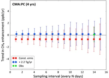
pro-file site calculated using a “background” over the North Pacific every N days (1 ≤°N ≤ 15) over 4 years. For a given sampling frequency, we estimated the possible range of observed trends by randomly choosing a time series starting point and introducing sampling gaps (with replacement) 50,000 times and then calculating the standard deviation of the ensemble of trends. Each trend was calculated byfitting a quadratic trend line and three harmonics through the sampled zonal gradient following Thoning et al. [1989]. For a given sampling duration, we consider the two emission scenarios distinguishable as long as the error bars do not overlap (equivalent in this case to requiring that the means differ by 2 standard deviations). We found that at CMA, a trend of 2.2 Tg CH4/yr2could be unambiguously detected in the zonal gradient of partial column CH4over
4 years, only if profiles are sample daily (Figure 5). This is significantly more frequent than the current
Figure 4. (top row) Full time series of simulated column average CH4differences between grid boxes containing the NOAA
aircraft monitoring sites, (left column) CMA and (right column) NHA, and a Pacific Ocean background (30–50°N, 135–125°W). Trends and uncertainties are shown for each case and are calculated using the method described in the text. (bottom row) Simulated column average CH4subsampled for locations of valid GOSAT nadir and glint background (30–50°N, 135–125°W)
soundings. The trends shown in the bottomfigures are calculated as a difference between the lines fit to the site and background column average CH4, similar to Turner et al. [2016].
sampling strategy of twice per month. Using an 8 year time series, subweekly sampling intervals were still needed for detection of the imposed trend. A similar result was found by Sweeney et al. [2015] con-cerning the observation frequency of profiles needed to accurately quantify U.S. fossil fuel CO2
emis-sions. Note that our choice of the partial column at a single site over 4 years was motivated by the need to explain the large trends in horizon-tal gradients shown in Figure 2. In practice, if we were to use multiple aircraft sites within the NOAA net-work in a source-sink inversion, over a longer time period, we could possi-bly detect an O&G emission trend as large as 2.2 Tg CH4/yr2with less fre-quent sampling. It is therefore impor-tant to make use of information from the entire network.
3.3. The Effect of Background Column Average CH4on Relative Trends
Although we have shown that infrequent sampling can cause spurious trends, we have not yet completely accounted for the large positive trends shown in Figure 2, since spurious trends in principle could be either negative or positive. The choice of the upstream background is another factor to consider, and Figure 6 shows that using a large region of the North Pacific as the background rather than a small offshore region as we did in section 3.2, following Turner et al. [2016], results in relative trends for both sites that are similar to those shown in Figure 2. There are two reasons for the large influence of the background chosen by Turner et al. [2016]: the large extent of their background area increased sensitivity to interannual variability in transport (Figure 3), and they were not able to account for spatiotemporal variability in the CH4seasonal
cycle. Due to the seasonal coverage bias of GOSAT glint and higher-latitude zenith soundings, it is not always possible to deseasonalize the zonal gradient of GOSAT column average CH4. NOAA aircraft profiles, however, do not have a seasonal sampling bias and are usually sampled at least twice per month. The trends in the
Figure 5. Simulated 4 year relative trends in partial column average CH4as a
function of sampling frequency for the grid boxes containing the NOAA air-craft monitoring site at CMA using an offshore Pacific Ocean background (30–50°N, 135–125°W). Trends and uncertainties are shown for Case 1 (repeating or“constant” emissions (red)) and Case 2 (as for Case 1 but with a 2.2 TgCH4/yr2trend in U.S. O&G emissions (blue)). The trend calculated using
NOAA aircraft profiles at CMA is also shown (green), where the error bars denote uncertainty using a bootstrap analysis of the observed profiles. Model simulations were performed at 1 × 1° spatial resolution.
Figure 6. Simulated column average CH4for the grid box containing the NOAA aircraft monitoring sites at (left) CMA and
(right) NHA (green), and for glint retrievals of North Pacific Ocean background column average CH4(blue). Background
column average CH4is defined as in Turner et al. [2016] (25–43°N, 176–128°W) (blue). The trends are calculated as a
aircraft-based partial column CH4at CMA compared to (a) an empirical north-south distribution derived from
interpolated in situ observations and (b) a marine boundary layer constructed from surface observations over 2010–2013 are 0.9 ± 1.4 ppb/yr and –1.3 ± 1.8 ppb/yr, respectively, if the zonal difference is not deseasona-lized. If, however, the zonal difference is deseasonalized before estimating a trend, the estimated trends are 0.2 ± 1.30 ppb/yr and 0.5 ± 1.15 ppb/yr, smaller than before and more consistent. Lack of information about the seasonal cycle may result in misleading trends in large-scale horizontal gradients
3.4. Detectability of Emission Trends From Vertical Gradients
We have shown in the preceding sections that large trends in zonal CH4gradients can arise purely from inter-annual variability in atmospheric transport, spatial and temporal sampling patterns, choice of“background” column average CH4, and variability of the seasonal cycle over short times, even when the underlying
emis-sions are not changing. This raises the question of whether there is a different spatial gradient that is more sensitive to trends in emissions that could be used to confirm or falsify a hypothetical emission trend. In this section, we look at the vertical gradient of CH4, defined as the difference between CH4mixing ratios between the planetary boundary layer (PBL, 0.2–2.5 km above ground level) and the free troposphere (FT, 5.0–8.0 km above sea level), at several sites across the continental U.S. where vertical profiles of CH4 are
regularly measured.
Since all CH4sources are at the surface, its abundance is typically enhanced in the boundary layer, and the vertical gradient can be expected to increase with time if local emissions increase. However, even in the absence of an emission trend, the vertical gradient could show trends over short periods due to interannually varying transport, much like zonal gradients discussed earlier. To analyze the sensitivity of vertical gradient trends to emission trends, we simulate the vertical gradient of CH4using the TM5 transport model for the
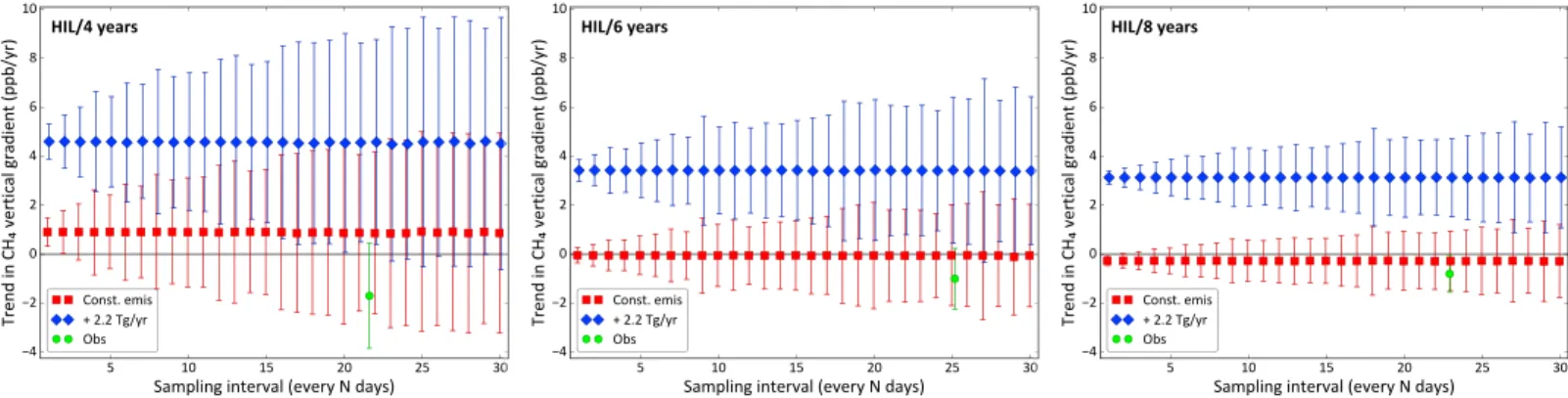
two emission scenarios, viz., with and without an emission trend of 2.2 Tg CH4/yr2 over 2004–2010 from O&G production. At any given aircraft profiling site, the ability to distinguish between the two emission sce-narios depends on over how long a period and how often the vertical gradient is sampled, as well as how sensitive the site is to changing emissions. To explore this parameter space, we sample the modeled vertical gradient at a site every N day(s) where N goes from 1 to 15, with time series lengths of 4, 6, and 8 years using the analysis described in section 3.2. The results of this calculation at the Homer, Illinois (HIL) site are shown in Figure 7.
Figure 7 shows that for a given sampling frequency and length of record, thefitted trend to the sampled ver-tical gradient for a given emission scenario can have a range of values, due to the inherent variability of the atmospheric CH4field. This range of possible trends (denoted by vertical error bars in Figure 7) decreases as
the sampling frequency and duration increases. As before, for a given sampling duration we consider the two emission scenarios distinguishable as long as the error bars do not overlap. For example, at HIL, if we sample over 6 years, then the two emission scenarios are distinguishable as long as the average interval between two profiles is about 15 days or less. If we sample for only 4 years, however, we need to sample at least every
Figure 7. Simulated trends in the vertical gradient of CH4at the NOAA aircraft site at Homer, Illinois (HIL) for three time series lengths (4, 6, and 8 years). For a given
sampling frequency, the error bars denote the range within which a trendfitted to sampled vertical gradients will lie 68% of the time. The two symbols represent the two emission scenarios, with an O&G emission trend of 2.2 Tg CH4/yr2(blue diamonds) and zero emission trend (red squares). Trends calculated using actual NOAA
5 days to tell the two scenarios apart. At the current sampling frequency, which is approximately once every 3 weeks, an 8 year time series is adequate to distinguish between the trend and no-trend simulations, and it is clear that the observations at HIL (green symbols, Figure 7) do not support a 2.2 Tg CH4/yr2trend.
This analysis is restricted to a single site. In practice, a trend in emissions will impact the vertical gradient at a site depending on its proximity to the emissions. Among the sites we looked at (Figure 8), the vertical gradi-ent changed appreciably at SGP, CAR, and HIL, and at these sites it is clear that the observed trends are more consistent with the zero trend case than the case with 2.2 TgCH4/yr2trend on O&G emissions. WBI appears to
be less sensitive to O&G emissions than HIL; however, the observed trend is larger and more negative, pos-sibly indicating the local importance of a non-O&G source process. There is significantly less sensitivity to changing O&G emissions at CMA and NHA, and time series much longer than 8 years would be required to detect even the large trend assumed for these simulations. This makes the intuitive point that sites closer to source regions can be used to detect emission trends more quickly, and raises the question of how best to combine observed gradient information from multiple sites, and if doing so would allow us to detect smal-ler trends, the same trend with less frequent sampling, or over a shorter time period. Such questions are best answered by an atmospheric inversion, which can deconvolve transport-related and emission-related varia-tions and infer surfaceflux trends from vertical gradients at multiple sites and lateral gradients between sites,
Figure 8. Simulated trends in the vertical gradient of CH4at NOAA aircraft sites Briggsdale, CO (CAR), Southern Great Plains, OK (SGP), West Branch, IA (WBI), Homer, Illinois (HIL), Worcester, MA (NHA), and Cape May, NJ (CMA) using 8 year time series. For a given sampling frequency, the error bars denote the range within which a trendfitted to sampled vertical gradients will lie 68% of the time. The two symbols represent the two emission scenarios, with an O&G emission trend of 2.2 Tg CH4/yr2(blue diamonds) and zero emission trend (red squares). Trends calculated using actual NOAA aircraft profiles over the same periods are shown in green circles, where the error bars denote uncertainty using a bootstrap analysis of the observed profiles.
in a statistically consistent manner. Note, however, that model transport biases are likely entrained in the results, but if a systematic bias does not change over time, a trend could still be detected.
4. Discussion
Atmospheric variability makes direct interpretation of trends in spatial gradients difficult, and we demon-strated that significant short-term relative trends can result purely from interannual variability in transport. Variability in transport is conflated with changes in emissions located outside of the U.S., and since U.S. O&G emissions are only about 2% of global total CH4 emissions [US EPA, 2016]; European Commission
[2011]) signals from changing US O&G emissions are likely to be difficult to detect without denser coverage of observations. Atmospheric variability ultimately plays a role in all of the detection issues we have dis-cussed: the need for high sampling frequency, the difficulty of defining a background, and accounting for short-term transport trends. The effect of atmospheric variability on trend detection has also been noted by other studies for ozone and carbon monoxide [Saunois et al., 2012; Strode and Pawson, 2013; Weatherhead et al., 1998, 2000]. Atmospheric modeling can be helpful because it can in principle account for transport variability. Future improvements in the ability of models to accurately simulate continental sites that are a challenge to model along with higher spatial and temporal resolution will make it possible to resolve more variability.
We have demonstrated that the trend of 2.2 Tg CH4/yr2for the period covering 2002–2014 in US O&G
emis-sions is inconsistent with an ensemble of global inversion estimates of CH4emissions. We have also shown
that the trends in the GOSAT column average CH4zonal gradient over North America seen by Turner et al. [2016] are not indicative of a trend in emissions. By simulating atmospheric CH4concentrations from a
repeating emission scenario, we have shown that spuriously large (up to ~4.5 ppb/yr) trends in GOSAT column average CH4zonal gradient can be caused by a combination of (i) interannual variability of transport over 4 years, (ii) seasonal sampling bias of GOSAT, (iii) choice of the North Pacific background, and (iv) not being able to account for variation in the seasonal cycle. The combination of these four artifacts make it difficult, if not impossible, to use zonal gradients of GOSAT column average CH4to detect and quantify a
trend in O&G emissions over short periods.
To determine whether trends in the zonal gradient of column CH4could in principle be used to distinguish an emission trend of 2.2 Tg CH4/yr2evenly distributed over U.S. O&G production regions from a case without an
emission trend, we looked at partial column CH4constructed from NOAA aircraft profiles. These data do not suffer from artifact (ii), and in principle could be rid of artifacts (iii) and (iv) by choosing a more appropriate background and deseasonalizing. However, we saw that over 4 years, the variability in the trend due to trans-port can overwhelm the expected signal from an emission trend, unless the frequency of profiles is increased significantly compared to what is currently possible. The variability due to transport goes down, and the detectability of an emission trend increases, if one considers trends in the zonal gradient over longer time periods. However, use of 8 year time series did not increase detectability.
Looking at vertical CH4profiles at NOAA aircraft locations, we have demonstrated that the trend in the
ver-tical gradient between the PBL and the FT may be a better indicator of an emission trend, compared to the zonal gradient sampled at the same frequency. This is especially true for profiles close to emission regions. At HIL, for example, we have shown that over 8 years, our current sampling frequency would be sufficient at dis-tinguishing a trend of 2.2 Tg CH4/yr2from a no trend case. In addition, our results for multiple sites show that the aircraft monitoring observations are consistent with zero change in U.S. O&G emissions.
Our conclusions above about the detectability of emission trends depend on aircraft profiles at a single site. If information from samples at multiple sites are combined in a statistically consistent way, such as in an atmo-spheric inversion, we expect the detectability to improve significantly, and the same emission trend may be detectable using less frequent sampling and over a shorter time.
The GOSAT satellite has a repeat cycle of 3 days over any given location, and the spatial sounding density is much higher than the current network of in situ sampling sites. In the absence of clouds and other confound-ing factors which lead to failed retrievals, column average CH4from GOSAT could in principle be used in an atmospheric inversion to detect trends in emissions. In practice the frequency of successful retrievals is much smaller than the frequency of soundings, and biases in GOSAT retrievals of column average CH4can be of the
order of 10 ppb [Alexe et al., 2015; Butz et al., 2011; Parker et al., 2011] and spatially coherent over large areas. It remains to be seen whether, given these limitations, GOSAT retrievals can be sensitive to trends in zonal gra-dients of the order of 1 ppb/yr, consistent with expected trends in CH4emissions. Before systematic biases
can be removed, they need to be quantified. This requires much more densely spaced soundings and thor-ough comparison with calibrated in situ data than what is currently possible. In the optimistic case that GOSAT retrievals are sensitive to such small trends despite their noise and bias, they are still limited to low latitudes. As seen in Figure 6 (right), even at 45°N GOSAT has very few successful retrievals. In order to impose constraints on surfacefluxes through the entire year over regions important for CH4fluxes, any source-sink inversion using GOSAT retrievals will also need to include in situ observations.
Atmospheric inversions, in principle, can combine information from multiple sites and account for atmo-spheric variability not related to surfacefluxes by explicitly modeling atmospheric transport. However, trends influxes derived from atmospheric inversions over short periods may still be unreliable, since transport varia-bility especially at small scales and high frequencies may not be well represented by the underlying transport model. Sparse atmospheric sampling in the form of observations is also a problem, since in the absence of observations inverse models revert back to priorfluxes; therefore, improved prior flux estimates would also be helpful for producing better posteriorflux estimates. An inaccurate trend in posterior fluxes may therefore also arise from an inaccurate trend in the prior combined with insufficient observations. Changes in colocated emissions from different sources also pose problems for attribution of emission changes, and observations of coemitted species may be particularly useful for source attribution. Sparse observations may also result in spatial misattribution of signals, and a trend in emissions can be spread over multiple source regions. Therefore, for confirming a trend in emissions from inverse models, it is advisable to look over a long time (a decade or so) at multiple inverse models spanning a wide spectrum of transport models, priorfluxes, and ingested observations. We looked at such an ensemble of inverse models in section 2 and found that none of them suggests a trend in U.S. CH4emissions since 2000 that is as large as 2.2 Tg/yr2.
The trade-offs we discussed between sampling frequency, length of time, and spatial density needed to detect changes in emissions have important policy implications. There is clearly a need to be able to detect short-term changes in emissions. Accomplishing that will require a continued commitment to frequent and dense sampling from a combination of platforms.
References
Alexe, M., et al. (2015): Inverse modeling of CH4 emissions for 2010–2011 using different satellite retrieval products from GOSAT and SCIAMACHY, Atmos. Chem. Phys., 15, 113–133. [Available at http://www.atmos-chem-phys.net/15/113/2015/acp-15-113-2015.pdf.] Alvarez, A. R., S. W. Pacala, J. J. Winebrake, W. L. Chameides, and S. P. Hamburg (2012), Greater focus needed on methane leakage from
natural gas infrastructure, Proc. Natl. Acad. Sci. U.S.A., 109(17), 6435–6440, doi:10.1073/pnas.1202407109. AMAP Assessment (2015), Methane as an Arctic Climate Forcer, AMAP, Oslo.
Bergamaschi, P., et al. (2015), Top-down estimates of European CH4and N2O emissions based on four different inverse models, Atmos. Chem.
Phys., 15, 715–736, doi:10.5194/acp-15-715-2015.
Bousquet, P., et al. (2006), Contribution of anthropogenic and natural sources to atmospheric methane variability, Nature, 443, 439–443, doi:10.1038/nature5132.
Bruhwiler, L., E. Dlugokencky, K. Masarie, M. Ishizawa, A. Andrews, J. Miller, C. Sweeney, P. Tans, and D. Worthy (2014), CarbonTracker-CH4:
An assimilation system for estimating emissions of atmospheric methane, Atmos. Chem. Phys., 14, 8269–8293, doi:10.5194/acp-14-8269-2014.
Butz, A., et al. (2011), Toward accurate CO2and CH4observations from GOSAT, Geophys. Res. Lett., 38, L14812, doi:10.1029/2011GL047888.
Dlugokencky, E. J., P. M. Lang, A. M. Crotwell, K. A. Masarie, and M. J. Crotwell (2015), Atmospheric methane dry air mole fractions from the NOAA ESRL carbon cycle cooperative global air sampling network. [Available at ftp://aftp.cmdl.noaa.gov/data/trace_gases/ch4/flask/ surface/.]
Dlugokencky, E. J., E. G. Nisbet, R. Fisher, and D. Lowry (2011), Global atmospheric methane: Budget, changes and dangers, Phil. Trans. R. Soc. A, 369, 2058–2071, doi:10.1098/rsta.2010.0341.
European Commission (2011), Joint Research Centre (JRC)/Netherlands Environmental Assessment Agency (PBL), Emission Database for Global Atmospheric Research (EDGAR), release version 4.2. [Available at http://edgar.jrc.ec.europa.eu.]
Franco, B., et al. (2016), Evaluating ethane and methane emissions associated with the development of oil and natural gas extraction in North America, Environ. Res. Lett., 11, 044,010, doi:10.1088/1748-9326/11/4/044010.
Frankenberg, C., I. Aben, P. Bergamaschi, E. J. Dlugokencky, R. van Hees, S. Houweling, P. van der Meer, R. Snel, and P. Tol (2011), Global column-averaged methane mixing ratios from 2003 to 2009 as derived from SCIAMACHY: Trends and variability, J. Geophys. Res., 116, D04302, doi:10.1029/2010JD014849.
Hausmann P., R. Sussmann, and D. Smale (2016), Contribution of oil and natural gas production to renewed increase of atmospheric methane (2007–2014): Top-down estimate from ethane and methane column observations, Atmos. Chem. Phys., 16, 3227–3224, doi:10.5194/acp-16-3227-2016. [Available at www.atmos-chem-phys.net/16/3227/2016/.]
Helmig, D., et al. (2016), Reversal of global trends in atmospheric ethane and propane from North American oil and gas production, Nat. Geosci., 9, 490–495, doi:10.1038/ngeo2721.
Acknowledgments
The authors acknowledge the efforts of the Global Carbon Project methane to produce and distribute the global methane budget on the CDIAC website: http://cdiac.ornl.gov/GCP/methanebud-get/2016/ (doi:10.3334/CDIAC/ Global_Methane_Budget_2016).
Houweling, S., et al. (2014), A multi-year methane inversion using SCIAMACHY, accounting for systematic errors using TCCON measure-ments, Atmos. Chem. Phys., 14, 3991–4012, doi:10.5194/acp-14-3991-2014.
Kaplan, J. O. (2002), Wetlands at the last glacial maximum: Distribution and methane emissions, Geophys. Res. Lett., 29(6), 1079, doi:10.1029/ 2001GL013366.
Kirschke, S., et al. (2013), Three decades of global methane sources and sinks, Nat. Geosci., 6, 813–823, doi:10.1038/ngeo1955.
Krol, M., S. Houweling, B. Bregman, M. van den Broek, A. Segers, P. van Velthoven, W. Peters, F. Dentener, and P. Bergamaschi (2005), The two-way nested global chemistry-transport zoom model TM5: Algorithm and applications, Atmos. Chem. Phys., 5, 417–432, doi:10.5194/acp-5-417-2005.
Kuze, A., H. Suto, M. Nakajima, and T. Hamazaki (2009), Thermal and near infrared sensor for carbon observation Fourier-transform spec-trometer on the Greenhouse Gases Observing Satellite for greenhouse gases monitoring, Appl. Opt., 48, 6716–6733.
Lin, J. C., C. Gerbig, S. C. Wofsy, A. E. Andrews, B. C. Daube, K. J. Davis, and C. A. Grainger (2003), A near-field tool for simulating the upstream influence of atmospheric observations: The Stochastic Time-Inverted Lagrangian Transport (STILT) model, J. Geophys. Res., 108(D16), 4493, doi:10.1029/2002JD003161.
Locatelli, R., P. Bousquet, M. Saunois, F. Chevallier, and C. Cressot (2015), Sensitivity of the recent methane budget to LMDz sub-grid-scale physical parameterizations, Atmos. Chem. Phys., 15, 9765–9780, doi:10.5194/acp-15-9765-2015. [Available at www.atmos-chem-phys.net/ 15/9765/2015/.]
Miller, S. M., et al. (2013), Anthropogenic emissions of methane in the United States, Proc. Natl. Acad. Sci. U.S.A., 110(50), 20,018–20,022, doi:10.1073/pnas.1314392110.
Monteil, G., S. Houweling, A. Butz, S. Guerlet, D. Schepers, O. Hasekamp, C. Frankenberg, R. Scheepmaker, I. Aben, and T. Röckmann (2013), Comparison of CH4inversions based on 15 months of GOSAT and SCIAMACHY observations, J. Geophys. Res. Atmos., 118, 11,807–11,823,
doi:10.1002/2013JD019760.
Nehrkorn, T., J. Eluszkiewicz, S. C. Wofsy, J. C. Lin, C. Gerbig, M. Longo, and S. Freitas (2010), Coupled weather research and forecasting-stochastic time-inverted Lagrangian transport (WRF-STILT) model, Meteorol. Atmos. Phys., 107, 51–64, doi:10.1007/s00703-010-0068-x. Nisbet, E. G., et al. (2016), Rising atmospheric methane: 2007–2014 growth and isotopic shift, Global Biogeochem. Cycles, 30, 1356–1370,
doi:10.1002/2016GB005406.
Nisbet, E. G., E. J. Dlugokencky, and P. Bousquet (2014), Methane on the rise—Again, Science, 343, 493–496, doi:10.1126/ science.1247828.
Parker, R., et al. (2011), Methane observations from the Greenhouse Gases Observing SATellite: Comparison to ground-based TCCON data and model calculations, Geophys. Res. Lett., 38, L15807, doi:10.1029/2011GL047871.
Patra, P. K., et al. (2011), TransCom model simulations of CH4and related species: Linking transport, surfaceflux and chemical loss with CH4
variability in the troposphere and lower stratosphere, Atmos. Chem. Phys., 11, 12,813–12,837, doi:10.5194/acp-11-12813-2011. Patra, P.K., et al. (2013), The carbon budget of South Asia, Biogeosciences, 10, 513–527, doi:10.5194/bg-10-513-2013. [Available at http://www.
biogeosciences.net/10/513/2013/.]
Peischl, J., et al. (2015), Quantifying atmospheric methane emissions from the Haynesville, Fayetteville, and northeastern Marcellus shale gas production regions, J. Geophys. Res. Atmos., 120, 2119–2139, doi:10.1002/2014JD022697.
Peischl, J., et al. (2016), Quantifying atmospheric methane emissions from oil and natural gas production in the Bakken shale region of North Dakota, J. Geophys. Res. Atmos., 121, 6101–6111, doi:10.1002/2015JD024631.
Peters, W., M. C. Krol, E. J. Dlugokencky, F. J. Dentener, P. Bergamaschi, G. Dutton, P. V. Velthoven, J. B. Miller, L. Bruhwiler, and P. P. Tans (2004), Toward regional-scale modeling using the two-way nested global model TM5: Characterization of transport using SF6, J. Geophys.
Res., 109, D19314, doi:10.1029/2004JD005020.
Philander, S. G. (1990), El Niño, La Niña and the Southern Oscillation, Academic Press, San Diego, Calif.
Saunois, M., L. Emmons, J.-F. Lamarque, S. Tilmes, C. Wespes, V. Thouret, and M. Schultz (2012), Impact of sampling frequency in the analysis of tropospheric ozone observations, Atmos. Chem. Phys., 12, 6757–6773, doi:10.5194/acp-12-6757-2012.
Saunois, M., et al. (2016), The global methane budget: 2000–2012, Earth Syst. Sci. Data, 8, 697–751, doi:10.5194/essd-2016-25.
Schaefer, H., et al. (2016), A 21st century shift from fossil-fuel to biogenic methane emissions indicated by13CH4, Science, 352(6281), 80–4,
doi:10.1126/science.aad2705.
Schwietzke, S., et al. (2016), Upward revision of global fossil fuel methane emissions based on isotopic database, Nature, 538, 88–91, doi:10.1038/nature19797.
Strode, S. A., and S. Pawson (2013), Detection of carbon monoxide trends in the presence of interannual variability, J. Geophys. Res. Atmos., 118, 12,257–12,273, doi:10.1002/2013JD020258.
Sweeney, C., et al. (2015), Seasonal climatology of CO2across North America from aircraft measurements in the NOAA/ESRL Global
Greenhouse Gas Reference Network, J. Geophys. Res. Atmos., 120, 5155–5190, doi:10.1002/2014JD022591.
Thoning, K. W., P. P. Tans, and W. D. Komhyr (1989), Atmospheric carbon dioxide at Mauna Loa Observatory 2. Analysis of the NOAA GMCC data, 1974–1985, J. Geophys. Res., 94(D6), 8549–8565, doi:10.1029/JD094iD06p08549.
Turner, A. J., et al, (2015), Estimating global and North American methane emissions with high spatial resolution using GOSAT satellite data, Atmos. Chem. Phys., 15, 7049–7069, doi:10.5194/acp-15-7049-2015.
Turner, A. J., D. J. Jacob, J. Benmergui, S. C. Wofsy, J. D. Maasakkers, A. Butz, O. Hasekamp, and S. C. Biraud (2016), A large increase in US methane emissions over the past decade inferred from satellite data and surface observations, Geophys. Res. Lett., 43, 2218–2224, doi:10.1002/2016GL067987.
US Energy Information Administration (EIA) (2016). [Available at https://www.eia.gov/naturalgas/data.cfm#production, https://www.eia.gov/ petroleum/data.cfm#crude.]
US Environmental Protection Agency (EPA) (2016). [Available at https://www.epa.gov/ghgemissions/us-greenhouse-gas-inventory-report-1990-2014.]
van der Werf, G.R., J. T. Randerson, L. Giglio, G. J. Collatz, P. S. Kasibhatla, and A. F. Arellano, Jr., (2006), Interannual variability in global biomass burning emissions from 1997 to 2004, Atmos. Chem. Phys., 6, 3423–3441. [Available at www.atmos-chem-phys.net/6/3423/ 2006/.]
Weatherhead, E. C., et al. (1998), Factors affecting the detection of trends: Statistical considerations and applications to environmental data, J. Geophys. Res., 103(D14), 17,149–17,161, doi:10.1029/98JD00995.
Weatherhead, E. C., et al. (2000), Detecting the recovery of total column ozone, J. Geophys. Res., 105(D17), 22,201–22,210, doi:10.1029/ 2000JD900063.
Wecht, K. J., D. J. Jacob, C. Frankenberg, Z. Jiang, and D. R. Blake (2014), Mapping of North American methane emissions with high spatial resolution by inversion of SCIAMACHY satellite data, J. Geophys. Res. Atmos., 119, 7741–7756, doi:10.1002/2014JD021551.
Wilson, C., M. Gloor, L. V. Gatti, J. B. Miller, S. A. Monks, J. McNorton, A. A. Bloom, L. S. Basso, and M. P. Chipperfield (2016), Contribution of regional sources to atmospheric methane over the Amazon Basin in 2010 and 2011, Global Biogeochem. Cycles, 30, 400–420, doi:10.1002/ 2015GB005300.
Zavala-Araiza, D., et al. (2015), Reconciling divergent estimates of oil and gas methane emissions, Proc. Natl. Acad. Sci. U.S.A., 112(51), 15,597–15,602, doi:10.1073/pnas.1522126112.