HAL Id: tel-01814212
https://pastel.archives-ouvertes.fr/tel-01814212
Submitted on 13 Jun 2018
HAL is a multi-disciplinary open access archive for the deposit and dissemination of sci-entific research documents, whether they are pub-lished or not. The documents may come from teaching and research institutions in France or abroad, or from public or private research centers.
L’archive ouverte pluridisciplinaire HAL, est destinée au dépôt et à la diffusion de documents scientifiques de niveau recherche, publiés ou non, émanant des établissements d’enseignement et de recherche français ou étrangers, des laboratoires publics ou privés.
using Finite Element Model Updating on Digital Image
Correlation measurements : towards the application to a
non-local model
Francesco Bettonte
To cite this version:
Francesco Bettonte. Development of a parameter identification strategy using Finite Element Model Updating on Digital Image Correlation measurements : towards the application to a non-local model. Materials. Université Paris sciences et lettres, 2017. English. �NNT : 2017PSLEM022�. �tel-01814212�
THÈSE DE DOCTORAT
de l’Université de recherche Paris Sciences et Lettres
PSL Research University
Préparée à MINES ParisTech
Development of a parameter identification strategy using Finite
Element Model Updating on Digital Image Correlation
measure-ments: towards the application to a non-local damage model
Développement d’une stratégie d’identification des paramètres par
re-calage de modèle éléments finis à partir de mesures par corrélation
d’images: vers l’application à un modèle d’endommagement non local
École doctorale n
o
432
SCIENCES ET MÉTIERS DE L’INGÉNIEUR
Spécialité
SCIENCE ET GÉNIE DES MATÉRIAUX
Soutenue par
Francesco BETTONTE
le 13 novembre 2017
Dirigée par
Jacques BESSON
Encadrée par
Sylvia FELD-PAYET
COMPOSITION DU JURY :
Mme Véronique DOQUET Président du jury
Laboratoire de Mécanique des Solides Mme Anne-Sophie CARO
Rapporteur
Centre des Matériaux des Mines d’Alès M. Marc GEERS
Rapporteur TU Eindhoven M. Jean-Noël PÉRIÉ Examinateur
Institut Clément Ader M. Jacques BESSON Examinateur
Centre des Matériaux Mines ParisTech Mme Sylvia FELD-PAYET
Examinateur ONERA
M. David LÉVÊQUE Invité
Remerciements
Ce manuscrit rassemble le travail de ces trois dernières années de thèse. Bien que j’en sois l’auteur, cette réussite n’aurait pas été possible sans le support et la collaboration de nombreuses personnes, que je souhaite remercier ici.
Je remercie les membres du jury, pour avoir examiné mon travail et mené une discussion intéressante au cours de la soutenance. Merci en particulier à Marc Geers et Anne-Sophie Caro pour avoir accepté le rôle de rapporteur.
Je tiens ensuite à remercier infiniment mes encadrants Sylvia, Jacques et David, pour m’avoir accompagné tout au long de ce parcours, mais aussi pour m’avoir soutenu dans mes décisions. J’ai pris un vrai plaisir à travailler à leur côté. Je n’oublierai jamais la confiance qu’ils m’ont accordée en me choisissant pour cette mission quand l’apprentissage de la langue française aurait pu être considéré comme un frein. J’ai aussi un remerciement particulier pour Jean-Didier, qui a véritablement été mon Virgile de la programmation informatique. Merci pour tous ses conseils et nos discussions autour d’un café. Merci également à Yves et Guy, pour leur aide précieuse dans le domaine du traitement d’images.
Merci à tous mes collègues du bâtiment E4 à l’ONERA, pour leur sympathie et leurs remarques de qualité sur mon travail au cours des différentes présentations. Je remercie également mes collègues doctorants, à l’ONERA comme au du Centre des Matériaux, pour leur bonne humeur.
Merci à mes parents et ma famille, pour m’avoir toujours encouragé dans mes études, et pour tous leurs efforts pour me permettre de réussir jusqu’ici. Je remercie de la même manière Martine et Patrick pour m’avoir accueilli et m’avoir aidé à démarrer ma vie en France. Enfin et surtout, je tiens à remercier ma petite amie, Audrey, de m’avoir soutenu inconditionnellement pendant ces trois années.
T
ABLE OFC
ONTENTSTable of Contents v
Page
Introduction 1
1 Material and Experimental Methods 5
1.1 Material . . . 5
1.2 Digital Image Correlation . . . 6
1.3 Choice of the specimens geometries and test conditions . . . 9
1.3.1 Selected geometries . . . 9
1.3.2 Experimental procedure and setup . . . 11
1.4 Experimental Results . . . 14
1.4.1 Identification of the elasticity parameters . . . 14
1.4.2 Analysis of the macroscopic response . . . 15
1.4.3 Microscopic analysis and initial void volume fraction . . . 19
2 Numerical modelling of ductile failure within the finite strain framework 27 2.1 Elasto-Visco-Plastic behaviour . . . 27
2.1.1 Elastic deformation . . . 28
2.1.2 Plastic deformation . . . 28
2.1.3 Viscous deformation . . . 32
2.2 Damage behaviour . . . 32
2.2.1 Global and local approaches to fracture . . . 32
2.2.2 Damage evolution by void growth . . . 33
2.3 Finite Element approach . . . 34
2.3.1 The strain localization problem . . . 37
2.3.2 The volumetric locking problem . . . 40
3 Prescription of measured boundary conditions 43 3.1 Introduction . . . 43
3.2 Impact of noise on the solution of the equilibrium problem . . . 44
3.2.1 Analytical test case: elasticity problem under antiplane shear condition . . 44
3.2.2 Numerical test case including plasticity . . . 46
3.3 Noise filtering . . . 47
3.3.1 Data reconstruction . . . 48
3.3.2 Mechanical filtering . . . 53
3.4 Discussion . . . 57
3.4.2 Experimental boundary conditions . . . 63
3.5 Conclusion . . . 65
4 Finite Element Model Updating 69 4.1 Parameter identification . . . 69
4.2 Parameter identification from full field measurements . . . 70
4.2.1 Constitutive Equation Gap method (CEG) . . . 70
4.2.2 The Virtual Fields Method (VFM) . . . 70
4.2.3 The Equilibrium Gap Method (EGM) . . . 71
4.2.4 The Finite Element Model Updating method (FEMU) . . . 71
4.3 Cost function . . . 74
4.4 Identification of parameters within the plastic regime . . . 76
4.4.1 Identification of the hardening parameters . . . 76
4.4.2 Verification of the hardening parameters . . . 78
4.4.3 Identification of the Hosford exponent . . . 83
4.5 Conclusion . . . 84
5 Identification of damage parameters via FEMU 87 5.1 Identification of the GTN model within the literature . . . 87
5.2 Influence of the regularization parameter . . . 88
5.3 Application of FEMU . . . 89
5.3.1 Identification . . . 89
5.3.2 Verification . . . 91
5.4 Validation of the damage parameters . . . 95
5.4.1 Validation on the first group of specimens . . . 95
5.4.2 Validation on the second group of specimens . . . 99
Conclusion and Perspectives 109 A Characteristics of the studied Inconel 625 113 B Comparison of the experimental displacement fields with their simulated coun-terparts 115 B.1 Alignment of the experimental (DIC) and numerical (FE) spatial coordinates systems115 B.2 Uncertainty of the matching uncertainty . . . 116
B.3 Values interpolation . . . 118
C Minimization of the cost function 119 D Validity of the asymptotic development 121 E Sensitivity analysis 123 E.1 Methodology . . . 124
E.2 Results . . . 124
E.2.1 Plasticity parameters . . . 124
E.2.2 Damage parameters . . . 130
I
NTRODUCTIONGeneral context
The use of numerical simulation into the industrial domain allows both to fasten the product development process and to reduce the prototyping costs. As a transfer institute, ONERA1, the French aerospace lab, has notably the mission of developing accurate numerical models for the simulation of damage and fracture. In particular, a recent research axis has been the development of regularized damage models. Their use is essential to the correct simulation of the softening behaviour of a structure. Indeed, regularization allows to overcome the well known problem of spurious localization with standard finite element formulations. This problem has been tackled notably through the doctoral works of Germain [49] and Feld-Payet [44], which mainly focused on the numerical aspects. In parallel, the doctoral works of Cuvilliez [35] and Zhang [136] were carried out at Electricité de France (EdF R&D), addressing more the constitutive behaviour aspects. The present work is complementary to the mentioned theses. It aims at investigating the identification of the regularized model parameters.
It is possible to find within the literature several references aiming at characterizing dam-age models. However, the majority of applications concerns local damdam-age models and so, the identification leads to results specific to a particular mesh. Moreover, in most cases the iden-tification is based on punctual or macroscopic measurements, without using the potential of modern measurement techniques, as Digital Image Correlation (DIC), which provide full-field measurements. The interest of full-field measurements for the identification of damage resides in the possibility to measure phenomena occurring at a relatively small scale, as in the localization band. Furthermore, full-field measurements can be used to drive a finite element simulation by prescribing measured displacements as boundary conditions, ensuring a consistent comparison between simulation and experiment. Advanced techniques as the Integrated Digital Image Corre-lation (I-DIC) use a finite element mesh to perform the digital image correCorre-lation while ensuring the consistency of the result with an associated constitutive models. But in the present study, the idea is to work on DIC results previously obtained, independently of any assumption on the behaviour, by any DIC software algorithm.
This study is part of the 4-years long project PRF MECHANICS at ONERA, which aims at improving the dialogue between experiment and simulation by means of image analysis. The objective of this project is to build a modular software platform, called escale, dedicated to the dialogue between experiments and simulations. Thanks to the flexibility of the Python language, the platform provides a practical interface which allows the communication through NumPy data exchanges between DIC codes, finite element problem solvers and optimization algorithms.
Objective
The objective of this study is to propose a robust strategy for the characterization of plastic behaviour and damage up to the onset of fracture. The strategy uses both load and DIC mea-surements. It is developed into a non-local damage framework. The identification is carried out considering a FEMU technique, according to which the parameters are identified by minimizing the discrepancy between the experimental measurements and their simulated counterparts, issued of a finite element model representative of the tests in terms of geometry and boundary conditions. Although several applications of FEMU for the characterization of a mechanical model can be found within the literature (see chapter 4), the novelty of this study consists in the complex context of application: the ductile failure process. Indeed, the large deformations involved are challenging both for the measurement system and for the finite element simulation, which are run up to the onset of failure. To assess the validity of the approach, the technique is applied to perform parameter identification on relatively simple specimens, and the parameters are used to simulate the response of complex geometries, which are then validated by comparison with the experimental responses.
Numerical tools
The DIC results are obtained by means of an efficient stereo correlation algorithm, FOLKI-D developed at ONERA [76]. Beyond the performances of the GPU implementation, the choice of FOLKI-D is motivated by the possibility of interacting with its developers to adapt the code in a relatively short delay. In fact, thanks to the necessities of parameter identification, the DIC software has been improved on several occasions.
The Finite Element results are obtained by means of Zebulon, an implicit solver co-developed by the École des Mines and ONERA. The finite strain formulation and the damage model are completely inherited from the PhD work of Zhang, mentioned above. It had been implemented within Zebulon at the beginning of the PhD and has been tested thanks to the identification needs.
The FEMU technique itself is implemented within escale. The development of escale was parallel to this thesis (no prior implementations of FEMU were available). Furthermore, the development of FEMU required the development of both the DIC and FE interfaces. Figure 0.1 illustrates the graphical interface of the platform, resulting from 3 years of developments, together with a significant result issued from the dialogue between experiment and simulation.
Approach of the thesis
Although the present work intends to provide a general approach for parameter identification applicable to any ductile metal undergoing large deformations, a unique material is considered in this work: the nickel-based superalloy Inconel 625. Ten different geometries (axisymmetric and flat) are selected to perform tensile tests, which are described in chapter 1. The choice of the geometries aims at obtaining heterogeneous displacement fields, in order to collect a maximum of information from Digital Image Correlation measurements. The selected geometries are tested up to failure, to create an experimental database adapted to the developments of this work.
The plastic behaviour of Inconel 625 is modelled using an Hosford yield criterion and a Voce-like isotropic hardening law, while damage evolution is modelled using a GTN damage model. The
finite element formulation is defined within the finite strain framework, considering a locking-free regularized formulation. Globally, the simulation of Inconel 625 relies on 16 parameters, including the regularization parameter of the non-local model, described in chapter 2.
The consistency of the comparison between experiment and simulation is ensured by the application of measured displacements as boundary conditions for the finite element problem, imposing the real kinematics of the deformation. However, the measured displacements need to be filtered, since the measurement uncertainty distorts the finite element solution, as described in chapter 3. An innovative filtering technique based on the Robin boundary condition is pro-posed and tested together with classical filtering approaches, as the moving least squares and polynomial approximations.
The discrepancy between experiment and simulation is quantified by means of a cost function, as described in chapter 4. The cost function, which represents the core difference between alternative FEMU approaches, is chosen to minimize both displacement and load. This is possible thanks to a proper normalization of each term. Before trying to minimize this cost function to identify the parameters, a preliminary sensitivity analysis is performed to determine a priori the feasibility of the identification by FEMU. Indeed, there might be a possible interaction between the parameters, leading to an indetermination on the result. The details of this analysis are presented in appendix E for both the plasticity parameters and the damage parameters.
Finally, the proposed identification approach is used to identify the GTN parameters on a flat geometry, as detailed in chapter 5. The resulting set of parameters is then used to obtain satisfactory simulations up to the onset of fracture for different geometries, confirming the validity of the approach.
Figure 0.1: The image shows 3 synchronized results: a DIC displacement field (left image) and its simulated counterpart obtained by prescribing measured displacements as boundary conditions on the top and bottom edges of the mesh (top right image), plus a comparison between the experimental force versus time curve and the simulated one (bottom right image) issued from a set of optimized parameters (see chapter 5).
Résumé
L’utilisation de la simulation numérique dans le domaine industriel permet d’améliorer le processus de développement, ainsi que de réduire les coûts de prototypage. L’ONERA, en tant qu’institut de transfert, a pour mission le développement de modèles numériques prédictifs pour la simulation de l’endommagement et de la rupture. Les thèses menées au cours de la dernière décennie se sont intéressées à la modélisation de l’endommagement dans un formalisme régularisé.
L’objectif de cette thèse, complémentaire aux précédentes, est de développer et mettre en œuvre une approche d’identification des paramètres pour un modèle d’endommagement régularisé. Cette approche utilise à la fois les efforts et les mesures de champ denses issues de la corrélation d’images. L’idée est d’utiliser la richesse des informations de ces mesures afin d’identifier des paramètres dont l’influence sur une structure est locale. L’approche d’identification proposée est fondée sur le recalage de modèle éléments finis (FEMU): les paramètres sont identifiés en minimisant l’écart entre une mesure expérimentale et son pendant simulé.
Bien que la méthode proposée soit applicable à divers matériaux, les travaux présents ont été réalisés sur l’alliage Inconel625. Les essais effectués ainsi que le choix des géométries sont illustrés dans le premier chapitre. Le deuxième chapitre est dédié à la modélisation du comportement et à la formulation éléments finis, choisis afin de reproduire le comportement observé expérimentalement. Le troisième chapitre introduit le dialogue essai-calcul. Sa fiabilité est garantie par l’application des déplacements mesurés comme conditions au bord pour le calcul éléments finis. Le chapitre met en évidence les problèmes issus de l’utilisation d’une donnée polluée par l’incertitude de mesure, et compare différentes techniques de filtrage. La méthode d’identification est clairement développée dans le quatrième chapitre et elle est appliquée pour l’identification des paramètres plastiques afin d’être validée. Enfin, le cinquième chapitre montre une application de la stratégie FEMU pour l’identification des paramètres d’endommagement.
C
H A P T E R1
M
ATERIAL ANDE
XPERIMENTALM
ETHODSThis chapter describes the experimental procedure and results that support the present PhD work. Parameter identification is performed using a FEMU technique on a set of tensile tests carried out at room temperature. The considered material, together with the motivations for its choice, are discussed in section 1. The kinematic full-field measurement considered in this work, are obtained using the Digital Image Correlation (DIC) technique described in section 2. The key point of the present work is the utilization of full-field measurements. In fact, they allow both to consider non-standard specimens for the characterization of the material and to get access to local variations of the kinematic response, such as those provoked by the damage phenomena. Hence, full-field measurements permit the identification of damage parameters, as done in [23, 110]. Moreover, the accuracy of the identification via FEMU is increased considering heterogeneous kinematic measurements as input for the inverse problem [7, 60]. Thus, the selection of the specimens geometry is an important phase, since the required kinematic heterogeneity is originated by means of geometrical heterogeneities such as notches and holes. Several works within the literature are focused on the determination of the more suitable geometries for parameter identification which maximize the heterogeneity of the kinematic fields (e.g. see [31, 37]). The choice of the geometries for the present tests is discussed in section 3, where the works of Dournaux [37] and Tanguy [126] are considered as guidelines. Finally, a micro-graphic analysis at the Scanning Electron Microscope (SEM) is performed on some selected specimens to evaluate the rupture mechanisms and to quantify the initial void volume fraction. The results are presented and discussed in section 4.
1.1
Material
Although the present work intends to provide a general approach for parameter identification applicable to any ductile metal undergoing large deformations, a unique material is considered in this work: the nickel-based superalloy Inconel 625. This alloy was developed in the early 1950’s to satisfy a growing demand for high-strength piping material [39]. Since then, thanks to some modifications of the chemical composition, the domain of application has been extended to the marine, nuclear and aerospace industry. The main characteristics of this material, which
motivated its choice as the reference material for this thesis, are the high tensile strength and the high deformation at break. Moreover, Inconel 625 shows also an high resistance to oxidation, which is here an advantage to perform fractographic analysis. Appendix A reports the chemical composition of the considered alloy and illustrates the microstructure.
1.2
Digital Image Correlation
Several techniques for measuring full-field kinematic fields (e.g. displacement) have been proposed in the literature during the last decades. Their main difference relies on the physical phenomena involved into the measurement approach. References [51, 54] provide an extended review of such techniques. The present work considers Digital Image Correlation (DIC), a white light technique, developed since the early 70s, which is becoming a standard tool in experimental mechanics [134]. In particular, the present work is concerned with local DIC methods, which provide a measure of the displacement fields without any assumption on the kinematics (as done for global DIC methods). The principle of image correlation is quite intuitive to understand. It consists in identifying the displacement of a deforming object by measuring the variation of light flow (the gray-level) between two consecutive images. It comes down to an optimization problem that is solved subset by subset (see figure 1.1). Thus, the object into the image should be characterized by a recognizable pattern. For this reason, metallic tensile test specimens (which are generally bright and smooth) are painted to generate a random speckle as in figure 1.1. The matching
Reference image Deformed image
u(x,y)
x
y
Figure 1.1: Principle of image correlation. The considered subset is the the red square. The measurement problem is solved when the pattern of all the subsets in the reference images is recognized within the deformed image (matching).
process is usually guided by a correlation measure, also referred to as score. A simple score would be the Sum of Squared Differences (SSD) which is the squared norm of the vector made by collecting the differences of gray-level between the pixels of each subset. Many references, as [105], use more robust scores, such as the Zero-centered Normalized Cross Correlation (ZNCC) to account for uncontrolled variations of the gray-scale level between images, for instance due to a difference of illumination. The measured displacement is then obtained by an optimization
1.2. DIGITAL IMAGE CORRELATION
process on the score (maximization or minimization depending on the chosen score). Several algorithms have been proposed for this optimization, which is an important computational burden considering the large images available nowadays. The image correlations of the present work are carried out using a correlation algorithm developed at ONERA, referred to as FOLKI-D1[76]. It is derived from a previously published algorithm for Particle Image Velocity (PIV), which in turn is derived from an algorithm for optical flow estimation [75]. The choice of FOLKI-D is motivated by the following (unordered) reasons:
• no post-filtering operations are carried out;
• the result is dense: displacement is estimated for each pixel of the image;
• the algorithm is well suited for parallel computation: the GPU implementation available within the escale platform at ONERA allows fast and accurate computing;
• the use of a non commercial software allows an ongoing development of the software and a better management of each step;
• the level of uncertainty of the measurement is generally low [76].
There are some major particularities that distinguish FOLKI-D from other correlation algo-rithms. In fact, only translation is considered as motion model between pixels. This might seem an heavy restriction, but the dense computation carried out allows to bypass the problem, leading to measure complex movements, as rotations, with a satisfactory accuracy [76]. Furthermore, FOLKI-D does not rely on an exhaustive research for the optimum, which would require a large number of score evaluations, often accelerated by FFT (Fast Fourier Transformation) in other algorithms. Instead, the score function is considered as a surface and a minimum (or maximum) is searched via a gradient-based approach. Furthermore, FOLKI-D uses a coarse-to-fine strategy based on a pyramid of images to avoid the optimization to stop on local minima (see figure 1.2). Starting from the original image (the largest one of the pyramid) low-pass filtering and down-sampling is performed to obtain smaller images. The downsampled images form the levels of the pyramid. The first estimation of the displacement field is done at the highest level of the pyramid (smallest image), considering a null displacement as initialization. Afterwards, the previous displacement estimation is expanded (upsampling) and used to initialize the correlation at the lower level of the pyramid. This latter process is repeated until the lowest level (the original image) is reached. Further details about FOLKI-D and its parallel implementation are given in [76].
Measuring large displacements The subset matching is a local operation. Hence, in case
the difference between the images is too important, the correlation might not succeed. However, the coarse-to-fine strategy native of FOLKI-D allows to estimate large displacements since the difference between the images at the top level of the pyramid is considerably reduced (of a factor 2(n−1), where n is the number of levels of the pyramid). Thus, large displacements at the bottom level are seen as relatively small displacements at the top level.
Nevertheless, the coarse-to-fine strategy might still not be enough for very large displacements. This is the case for the current work. The solution to overcome this problem is to update the reference image (the zero load image) with an intermediary one and to perform an intermediary
Figure 1.2: Pyramid of images. Starting from the lower level of the pyramid (the original image) the higher levels are obtained obtained by downsampling the image of the previous level. Once the pyramid is created, the correlation begins at highest level (the smallest image) and the result of each level is used to initialize the correlation at the lower level of the pyramid, until the bottom is reached.
correlation. Afterwards, this latter result is combined with the previous ones in order to obtain a Lagrangian description of displacement. However, the combining operation involves interpolation of data and so, it might be a source of errors. Therefore, it should be used only when necessary, i.e. when a direct correlation would not work. In order to assess the error introduced by the combining operation, the resulting DIC displacements have been compared with the displacements measured by a calibrated extensometer. A smooth cylindrical specimen was considered for this operation. Figure 1.3 shows that the relative error in the worst case scenario (the combining operation is performed for each image step) is lower than 1.2%.
Quality of the measure The quality of the measured displacement fields can be assessed
using by-products of the FOLKI-D iteration. A first indicator is the final score coefficient, which is related to the validity of the matching operation. A correct matching indicator in experimental mechanics should be higher than 90%. A second indicator of the precision is the standard deviation, or uncertainty, of the displacement field. It can be computed using the final Hessian of the optimization procedure and the variance of the residual image, as described in [76]. Many factors influences the uncertainty, as the illumination or the distance of the specimen from the camera. However, the average uncertainty of the measures carried out during the present work is of the order of ±1µm for the in-plane displacements and 2µm for the out-of-plane displacements.
Stereoscopic DIC Stereo DIC is used in the present work. In stereo DIC two images are
recorded at each instant. Thanks to the geometrical calibration, conducted using the AFIX2 software available at ONERA [77, 78], the FOLKI-D algorithm is used to compute the disparity map, for each each time step. The disparity allows to reconstruct the 3D surface of the sample and also to project the images of the second camera onto the pixel grid of the first camera to perform a temporal correlation afterwards.
1.3. CHOICE OF THE SPECIMENS GEOMETRIES AND TEST CONDITIONS
0
50
100
150
200
250
300
350
400
Image number
0.0
0.2
0.4
0.6
0.8
1.0
1.2
Error %
Combine: 400 updates
Combine: 120 updates
Combine: 40 updates
Figure 1.3: Evaluation of the error introduced by the combining operation. The reference image has been updated in different ways from an update at each step (400 for 401 images), unreasonable and unnecessary, to a more reasonable value (40 for 401 images). The relative error has a maximum value of around 1.2% for the worst case scenario.
1.3
Choice of the specimens geometries and test conditions
As introduced, the main guideline for the selection of the specimens geometries should be the level of heterogeneity of the kinematic fields. Furthermore, the stress triaxiality level should be taken into account while studying ductile failure, since it drives damage evolution [126, 135]. Therefore, the mechanical tests are here carried out on various geometries inspired from the previous works of Dournaux [37] and Tanguy [126]. Four flat geometries and four cylindrical geometries are retained. Nevertheless, flat (and relatively thin) specimens represent here the preferred choice to perform damage parameter identification from full-field measurements. Indeed, for flat specimens, it is possible to suppose the mechanical fields (and in particular the stress triaxiality) constant along the thickness direction. Hence, what is measured on surface by DIC is representative of the response at the specimen’s core. However, cylindrical specimens are often used to study ductile failure [126] and including them in the present work allows to compare the results with previous works.
1.3.1 Selected geometries
The considered geometries are referred to by means of abbreviations which indicate their shape and notch severity. Notations C and P indicates whether the specimen is axisymmetric or flat, respectively. Notations SMOOTH, and AE indicates whether the specimen is smooth or notched, respectively. Finally, a number indicates the severity of the notch. Such a value is to be considered
as a relative quantity rather than an absolute one. One flat specimen differs considerably from the other since it induces a plain strain condition, and will be referred to as PDP. The sketches are reported in figures 1.4, 1.5 and 1.6. The dimension of the geometries has been computed by scaling and adapting the original dimensions to the 30 mm round bar available.
(a) CSMOOTH (b) CAE10
(c) CAE4 (d) CAE2
Figure 1.4: Axisymmetric geometries, inspired from reference [126]. All the geometries have the same cross section area. They allow to study ductile failure because of the high stress triaxiality level reached at core. Cracks propagate from the core towards the surface.
1.3. CHOICE OF THE SPECIMENS GEOMETRIES AND TEST CONDITIONS
(a) PSMOOTH (b) PAE2
(c) PAE1
Figure 1.5: Flat geometries, inspired from reference [37]. All specimens are 2 mm thick. Flat specimens are characterized by a lower stress triaxiality level compared to the axisymmetric geometries, but it can be supposed constant along the thickness direction. Cracks propagate from the notches towards the center.
R2,0 0 26,00 2, 00 4,00 4,00 R2 ,00 20 ,0 0 6, 00 24,00
Figure 1.6: PDP Plain strain geometry, inspired from reference [126]. Cracks propagate from the center towards the notches.
1.3.2 Experimental procedure and setup
Two identical cameras, which characteristics are summed up in table 1.1, where placed in front of each specimen to realize a stereoscopic vision system, that is visible in figure 1.7. The speckle on the specimens was realized by means of an airbrush, rather than a spray bomb, in order to avoid the splintering of the paint because of an incohesive paint layer.
All the mechanical tests were performed at room temperature on servo-hydraulic testing machines. Specimens were monotonously loaded at various displacement rates that induced local strain rates within the range 10−3− 10−4s−1. In addition, specimens CSMOOTH-4 and PAE2-2 were equipped with a large strain extensometer and some elastic unloads were performed in order to observe a possible loss of stiffness due to damage. Image recording was synchronized with the testing machine data sampling by means of Mecanismes, a software developed at ONERA. Table 1.2 summarizes the performed tests and their respective loading conditions.
Figure 1.7: Experimental set-up for tensile tests. The 2 camera form the stereoscopic vision system, while the spot light ensures a constant light flow preventing erroneous correlations.
Camera AVT MANTA G-235B
Sensor CMOS
Resolution 1936 × 1216 pixels
Objective Schneider-Kreuznach 50 mm
Dynamic range 8 bits
1.3. CHOICE OF THE SPECIMENS GEOMETRIES AND TEST CONDITIONS T est Images Machine Geometry T est number Loading Sampling Integration f f Name Sampling Rate mm/min -Mode Hz ms mm Hz Cylindrical Specimens C Smooth 1 0,8 -Monotonic 0,1 50 -60 50 MTS 810 2 C Smooth 2 0,8 -Monotonic 0,2 50 -60 50 MTS 810 2 C Smooth 3 5 -Monotonic 1 70 50 MTS 810 50 C Smooth 4 5 -Cyc le 1 70 50 MTS 810 50 5 mm + 7 x (0,15 mm unload + 2 mm load) C AE10 1 0,8 -Monotonic 0,3 50 -60 50 MTS 810 2 C AE10 2 0,08 -Monotonic 0,2 50 -60 50 MTS 810 2 C AE10 3 0,8 -Monotonic 1 50 -60 60 MTS 810 10 C AE4 1 0,04 -Monotonic 0,2 50 -60 50 MTS 810 2 C AE4 2 0,04 -Monotonic 0,2 50 -60 50 MTS 810 2 C AE2 1 0,4 -Monotonic 0,5 50 -60 60 MTS 810 10 C AE2 2 0,4 -Monotonic 1 50 -60 60 MTS 810 10 Flat Specimens P Smooth 1 2 -Monotonic 1 50 -60 50 f/4 LOS 10 P AE1 1 1,2 -Monotonic 0,5 50 -60 50 f/4 LOS 10 P AE1 2 1,2 -Monotonic 0,5 50 -60 50 f/4 Instron 5582 10 P DP 1 1,2 -Monotonic 1 50 -60 50 f/4 LOS 10 P AE2 1 1,2 -Monotonic 0,5 50 -60 50 f/4 LOS 10 P AE2 2 0,5 -Cyc le 1 50 -60 50 f/4 LOS 10 3 x (2 mm load + 0,2 mm unload) P AE2 3 1,2 -Monotonic 0,5 50 -60 50 f/4 MTS 810 10 T able 1.2: List of the tensile tests carried out. Some of the tests inc luded a fixed number of elastic unloads to investigate damage evolution. The prescribed displacement rate induces a local strain rate within the ra nge 10 − 3 − 10 − 4 s − 1 .
1.4
Experimental Results
The purpose of this section is to provide a first analysis of the tensile tests. The objective is to understand the behaviour of Inconel 625 to develop the identification protocol.
1.4.1 Identification of the elasticity parameters
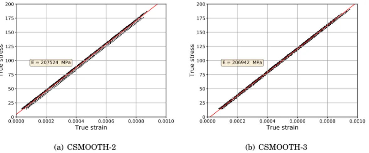
The identification of the elasticity parameters, i.e. the elastic modulus and the Poisson’s ratio, is not performed using FEMU in this study, although FEMU has already been successfully used for such a task [79, 121]. Therefore, the camera trig frequency was adapted for the plasticity and damage phenomena (see table 1.2), to concentrate the effort on the identification of the plasticity and damage parameters. The modulus of elasticity was measured by considering two of the tests on axisymmetric cylindrical specimens (CSMOOTH-2 and CSMOOTH-3). To do so, a small strain extensometer was used. The procedure involved 6 load cycles for each specimen (within the elastic regime). Three cycles were performed in displacement control (loading at a 0.8 mm/min rate up to an elongation of 0.08 mm) while the other three cycles were performed in load control (loading at a 0.85 kN/s up to an force of 5 kN). For each cycle, the elastic modulus were estimated by fitting a linear model (see figure 1.8) by means of the RANSAC2(random sample consensus) algorithm [45]. Finally, the average value of the 6 cycles was retained. The Poisson’s
0.0000 0.0002 0.0004 0.0006 0.0008 0.0010 True strain 0 25 50 75 100 125 150 175 200 True stress E = 207524 MPa (a) CSMOOTH-2 0.0000 0.0002 0.0004 0.0006 0.0008 0.0010 True strain 0 25 50 75 100 125 150 175 200 True stress E = 206942 MPa (b) CSMOOTH-3
Figure 1.8: Stress versus strain response of 6 cycles within the elastic range.
ratio was simply taken from the literature [1] since it has a negligible effect on the plasticity and damage phenomena. Table 1.3 reports the considered value for the elasticity parameters.
Young’s modulus E Poisson’s ratioν
207 GPa 0.308
Table 1.3: Elastic properties of Inconel 625 at room temperature. Young’s modulus is measured while the Poisson’s ratio is taken from the literature.
1.4. EXPERIMENTAL RESULTS
1.4.2 Analysis of the macroscopic response
The analysis of the macroscopic response provides information about the experimental scattering and any possible viscosity effect. Furthermore, damage could be quantified if a considerable variation of stiffness is measurable.
The large strain extensometer applied on specimens 3 and 4, together with a virtual exten-someter for specimen PSMOOTH-1, provides the stress-strain curves of figure 1.9.
0
10
20
30
40
50
60
L L0%
0
200
400
600
800
1000
F AM
0Pa
CS-3 - 5 mm/min
CS-4 - 5 mm/min
PS-1 - 2 mm/min
Figure 1.9: Tensile test response (stress versus strain) of smooth specimens. The experimental scattering due to the inhomogeneity of the raw material bars is considerable (the maximum discrepancy values approximatively 100 MPa).
Inconel 625 at the annealed state shows high deformation at break (over 50 %) at room temperature, a considerable hardening and a clear experimental scattering. Figure 1.10 shows the macroscopic responses of the axisymmetric specimens while figure 1.11 shows the macroscopic responses of the flat specimens. Let us first note that the experimental scattering observed on the smooth specimens is confirmed with the notched specimens. In fact, there is an obvious lack of repeatability of the experimental response for a test carried out twice (or more) at the same loading rate. A possible explanation of this scattering is that the various specimens comes from different slices of the original raw bar, for which the mechanical properties might be locally different. The second remark is about the viscous effect, which appears to be negligible at room temperature for the tested loading rates. In fact, as visible in figures 1.10(b) and 1.9, the same test carried out at different loading rates (of a factor 10 and 6 respectively) does not induce a significantly different macroscopic response. Let us observe that the number of tests performed is not high enough to precisely quantify the experimental scattering or to assess any viscous effect, which is not the purpose of the present work.
0 5 10 15 20 25 L mm 0 200 400 600 800 F A M0 Pa CS-1 - 0.8 mm/min CS-2 - 0.8 mm/min CS-3 - 5 mm/min CS-4 - 5 mm/min
(a) Unnotched specimen
0.0 0.5 1.0 1.5 2.0 2.5 3.0 L mm 0 200 400 600 800 1000 F A M0 Pa CAE10-1 - 0.8 mm/min CAE10-2 - 0.08 mm/min CAE10-3 - 0.8 mm/min (b) CAE10 0.0 0.5 1.0 1.5 2.0 2.5 L mm 0 200 400 600 800 1000 F A M0 Pa CAE4-1 - 0.04 mm/min CAE4-2 - 0.04 mm/min (c) CAE4 0.0 0.5 1.0 1.5 2.0 2.5 L mm 0 200 400 600 800 1000 1200 F A M0 Pa CAE2 - 1 - 0.4 mm/min CAE2 - 2 - 0.4 mm/min (d) CAE2
Figure 1.10: Mechanical response of the axisymmetric specimens. There is a observable lack of repeatability of the tests, especially within the plastic regime, and no evident viscous effects.
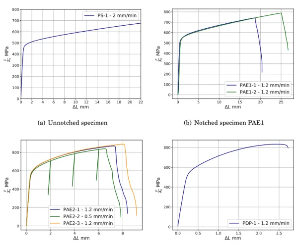
1.4. EXPERIMENTAL RESULTS 0 2 4 6 8 10 12 14 16 18 20 22 L mm 0 100 200 300 400 500 600 700 800 F A M0 Pa PS-1 - 2 mm/min
(a) Unnotched specimen
0 5 10 15 20 25 L mm 0 100 200 300 400 500 600 700 800 F A M0 Pa PAE1-1 - 1.2 mm/min PAE1-2 - 1.2 mm/min
(b) Notched specimen PAE1
0 2 4 6 8 L mm 0 200 400 600 800 F A M0 Pa PAE2-1 - 1.2 mm/min PAE2-2 - 0.5 mm/min PAE2-3 - 1.2 mm/min
(c) Notched specimen PAE2
0.0 0.5 1.0 1.5 2.0 2.5 L mm 0 200 400 600 800 F A M0 Pa PDP-1 - 1.2 mm/min
(d) Notched plain strain specimen PDP
Figure 1.11: Mechanical response of the flat and plain strain specimens. There is a remarkable scattering at failure. Let us note that the test on the smooth specimens was interrupted at a strain level of around 27% due to the machine maximum displacement restriction.
Measure of damage from loss of stiffness According to Lemaitre and Chaboche [81], any possible evolution of damage induces a loss of stiffness of the material. Therefore, the elastic unloads performed on test CSMOOTH-4 have been analysed. For each unload, the Young’s modulus was calculated supposing a small perturbation. When analysing the loss of stiffness, it is important to distinguish the loss of stiffness of the material due to damage from the loss of stiffness of the structure due to the geometric change imposed by deformation (deformation causes a progressive reduction of the resistant section). This distinction is simply made by calculating the Young’s modulus of the unloads respectively on the true and nominal stress-strain curve. Let us explicit the relations between nominal quantities and true quantities by means of the hypothesis of mass conservation, which is valid within the plastic regime. It will be shown that the stiffness of the structure decreases as a function of the nominal strain. In the following, notationsεindicates strain, notationσindicates stress and suffix n indicates a nominal quantity. Notations S and l refers to the cross section and specimen’s length respectively, while the suffix 0 denotes the initial value of the associated quantity. Hence, stress and strain are defined as:
(1.1) σn= F S0 σ= F S (1.2) εn=∆l l0 ε= l Z l0 1 ldl = ln µ 1 +∆l l0 
where imposing the mass conservation hypothesis S0l0= Sl, it gives the following expressions for the actual length and the actual cross section:
(1.3) l = l0+∆l = l0(1 +εn) S =
S0 1 +εn
which, in turn, give the relations between nominal quantities and true quantities:
(1.4) ε= ln(1 +εn) σ=σn(1 +εn)
At this point, to obtain the relation between the nominal stiffness and the true stiffness it is necessary to explicit the response of the system to a small perturbation of strain δε= ∆ul , supposing that it will induces a small perturbation of stressδσ=∆FS :
(1.5) E =δσ δε = ∆F ∆u l S= ∆F ∆u l0(1 +εn)2 S0 = δσn δεn(1 +εn )2= En(1 +εn)2
hence, the structure’s stiffness decreases, with respect to the material’s stiffness, according to:
(1.6) En=
E (1 +εn)2
Table 1.4 reports the stiffness for the performed unloads3. It is possible to note that while the nominal stiffness is decreasing because of the change of geometry, the true stiffness remains constant up to the last measured step. It means that it is not possible, in this case, to quantify damage by means of a variation of the elastic modulus. It may signify that failure happens mainly because of a strong late nucleation of voids.
3Let us note that the difference of the initial value with the previously measured value (see table 1.3) is to be
attributed to the lack of precision for small increments of strain of the large strain extensometer used. However, the relative comparison between each unloads remains valid.
1.4. EXPERIMENTAL RESULTS
* E MPa E (nominal) MPa εn [%]
Initial 192459 191791 0.1 Unload 1 189002 147572 13 Unload 2 188053 134126 18.2 Unload 3 189750 124061 23.4 Unload 4 189681 113738 28.7 Unload 5 189729 104995 34.1 Unload 6 190097 96863 39.7 Unload 7 190848 89481 45.6 Unload 8 191093 82350 51.9
Table 1.4: Elastic modulus for each elastic unload performed on the specimen CSMOOTH-4.
0.0
0.1
0.2
0.3
0.4
0.5
n
80
100
120
140
160
180
E,
E
n
[G
Pa
]
E
n
=
(1 +
E
n)
2E
E
n
Figure 1.12: Evolution of the nominal elastic modulus (En) and true elastic modulus (E) versus the nominal strain levelεn. There is no observable loss of stiffness of the material up toε≈ 52%, so that damage cannot be quantified in this manner. The apparent loss of stiffness showed by the nominal elastic modulus is attributed to the reduction of cross section due to deformation.
1.4.3 Microscopic analysis and initial void volume fraction
A part of the broken specimens was used to perform microscopic analysis. Both fracture surfaces and polished cross sections have been observed at the Scanning Electron Microscope (SEM). Fracture surfaces provide data about the rupture mechanisms, while cross sections allow to trace
the evolution of void volume fraction versus strain level. This latter analysis allows to determine an initial void volume fraction which is a key parameter for modelling damage evolution.
Fractography Let us begin the analysis with the fracture surfaces of CAE10-1 and CAE10-2,
visible in figure 1.13. They show a cup cone surface typical of ductile metals [126]. Furthermore, the circular shape of the flat fracture zone confirms the isotropic behaviour of Inconel 625. It is
(a) CAE10 - 1 (0.8 mm/min) (b) CAE10 - 2 (0.08 mm/min)
Figure 1.13: Fracture surface at macro scale of specimens CAE10-1 and CAE10-2. The cup-cone aspect of the surface is typical of ductile failure. The circular shape of the flat zone indicates an isotropic behaviour.
now interesting to observe the fracture surface at the scale of the grain size, considering that specimens CAE10-1 and CAE10-2 were tested at different (one order of magnitude) displacement rates. The specimen loaded at a higher displacement rate (CAE10-1, figure 1.14(a), loaded at 0.8 mm/min which induces a local strain rate of about 10−3s−1) shows transgranular fracture typical of ductile failure. Indeed, the fracture surface is characterized by the presence of large cavities (of about 10µm) initiated at inclusions. The specimens loaded at a lower displacement rate (CAE10-2, figure 1.14(b) loaded at 0.08 mm/min which induces a local strain rate of about 10−4s−1) show both intergranular and transgranular fracture. Indeed, in addition to the large cavities, the fracture surface is characterized by macro faults which size(about 20µm) is consistent with the average grain size. There might be possible relation between the strain rate and the failure mechanisms, as discussed in the PhD thesis of Max [95] where it is observed a change between intergranular and transgranular fracture as function of temperature and strain rate. This observation seems consistent with the fracture surfaces of axisymmetric specimens CAE4-1 and CSMOOTH-2 (see figure 1.15) and the fracture surfaces of the flat specimens PAE1-1 and PAE2-1 (see figure 1.16). The local strain rate of these latter 4 specimens was of the order of 10−4s−1. However, the relation between strain rate, stress triaxiality and fracture mechanism was not further investigated in the present work.
1.4. EXPERIMENTAL RESULTS
(a) CAE10 - 1 (0.8 mm/min) (b) CAE10 - 2 (0.08 mm/min)
Figure 1.14: Fracture surfaces observations of the notched specimen CAE10. The different loading rates generate different fracture surfaces. The specimen loaded at a higher rate (left) shows transgranular fracture, while the specimen loaded at a lower rate (right) shows, in addition, intergranular fracture. Images were taken near the centre of the fracture surface.
(a) CSMOOTH - 2 (b) CAE4 - 1
Figure 1.15: Fracture surfaces observations of the notched specimens CAE4-1 and CSMOOTH-2. The fracture surfaces are characterized both by intergranular fracture and transgranular fracture. Images were taken near the centre of the fracture surface.
(a) PAE1 - 1 (b) PAE2 - 1
Figure 1.16: Fracture surfaces observations of the notched specimens PAE1-1 and PAE2-1. The fracture surfaces are characterized prevalently by intergranular fracture. Images were taken near the centre of the fracture surface.
1.4. EXPERIMENTAL RESULTS
Measurement of the initial void volume fraction The analysis of the polished cross
sec-tion4 of the raw material allows to calculate the initial void volume fraction of the material. Furthermore, the same analysis performed on the cross sections of the broken specimens allows to trace the evolution of void volume fraction versus strain. From this latter, it is possible to extrapolate the value of void volume fraction at arbitrary values of strain. Three tests have been considered to perform this analysis (CAE10-3, PAE2-2, PSMOOTH-1).
The void volume fraction is quantified in terms of percentage of surface by an image thresh-olding operation. To distinguish voids from inclusions (all types confounded) the SEM was set to generate images where matrix, voids and inclusions correspond to three distinct gray levels as in figure 1.17. A regular grid of images(200µm wide, 10% overlap) has been created for each
Inclusion Matrix
Void 200 μm
Figure 1.17: Example of polished cross section (CAE10-3). Matrix, voids and inclusions correspond to three distinct gray levels. Although the void volume fraction might seem high, the majority of the dark spot are inclusions. The image has also been chosen as illustration to be particularly rich in dark spots, compared to the remaining images.
cross section, as in figure 1.18. Once the void volume fraction value f , and the inclusion ratio value r, were computed for each subset, the following relation has been used to fit the evolution of porosity versus the distance from fracture, denoted x (which is related to the strain level):
(1.7) f = ae−bx+ f0
4The cross section is realized by performing a cut along the loading direction (i.e. perpendicular to the fracture
~ 2 mm
Figure 1.18: Schema of regular grid on cross section (CAE10-3).
where x is the distance from the fracture surface. Coefficients a and b are two adjustable coefficients used to perform an exponential fit. Finally, coefficient f0 quantifies the void volume fraction at the opposite of the fracture surface. The choice of the constant parameter f0 allows to use equation 1.7 to fit constant profiles of void volume fraction (e.g. for the raw material). Therefore, parameter f0will be used to evaluate the void growth versus strain. Figure 1.19 shows the profiles of porosity and inclusions (which have been fit considering a constant value), while table 1.5 reports the coefficient f0 for the considered specimens and the relative strain level measured by DIC. Let us note that void growth is relatively low, since at a relative high strain level (35% for a deformation at break of 50%) void volume fraction is barely 5 times higher than the initial value, which is considerably low as well (1 · 10−4). This observation is consistent with the observation at macroscopic scale of table 1.4: void volume fraction is not high enough to induce an observable loss of stiffness of the material. Finally, let us note that the inclusion level is approximatively constant for the considered specimens.
1.4. EXPERIMENTAL RESULTS Specimen p0 ε% Raw Material 1 · 10−4 0 PAE2-2 1.8 · 10−4 10 PSMOOTH-1 3.7 · 10−4 27 CAE10-3 5.6 · 10−4 35
Table 1.5: void volume fraction for different specimens and the relative (approximative) strain level. The void volume fraction at relatively high strain level is moderate.
0.0000 0.0001 0.0002 0.0003 0.0004 0.0005 Porosity p0 = 1.0e-04 0 2 4 6 8 10 Images 0.000 0.001 0.002 0.003 0.004 Inclusion r = 2.4e-03
(a) Raw Material
0.0000 0.0005 0.0010 0.0015 0.0020 Porosity p0 = 1.8e-04 0 5 10 15 20 25 30 Images 0.000 0.001 0.002 0.003 0.004 Inclusion r = 2.3e-03 (b) PAE2 - 2 0.0000 0.0002 0.0004 0.0006 0.0008 0.0010 Porosity p0 = 3.7e-04 0 5 10 15 20 25 30 Images 0.000 0.001 0.002 0.003 0.004 Inclusion r = 2.1e-03 (c) PSMOOTH 1 Images 0.000 0.001 0.002 0.003 Voids ratio p0 = 5.5e-04 0 2 4 6 8 0.000 0.001 0.002 0.003 Inclusion r = 1.5e-03 (d) CAE10 - 3
Résumé
Ce premier chapitre présente l’approche expérimentale. Y sont décrits le choix des géométries, ainsi que la méthode de mesure par corrélation d’images et les premières observations sur les essais. Bien que la stratégie d’identification proposée dans cette thèse soit conçue pour tous les matériaux ductiles soumis à de grandes déformations, un seul matériau est utilisé pour mener l’étude. Il s’agit de l’alliage Inconel625, utilisé dans l’aéronautique.
La rupture ductile est fortement influencée par le niveau de triaxialité des contraintes. Afin de varier l’état de contraintes, les essais sont réalisés sur des éprouvettes entaillées avec différents rayons d’entaille. Outre les géométries axisymétriques habituellement utilisées pour l’étude de la rupture ductile, des géométries planes sont également prises en compte afin de tirer profit de la richesse des informations de la corrélation d’images. En effet, grâce à la faible épaisseur des éprouvettes planes, le niveau de triaxialité est quasi-constant dans l’épaisseur et l’amorçage de la fissure est visible en surface.
La corrélation d’images est faite grâce à un algorithme de corrélation local développé à l’ONERA. Les résultats fournis sont denses et non filtrés (lissage, etc.).
L’alliage étudié montre une rupture à un niveau important de déformation (≈ 50 % à l’ambiante) et une forte dispersion de la réponse macroscopique. Cette dispersion affecte davantage le domaine plastique pour les éprouvettes axisymétriques et l’instant d’amorçage de la fissure pour les éprouvettes planes. Dans tous les cas, la rupture suit rapidement l’amorçage et s’accompagne peu de striction.
Les observations au microscope à balayage (MEB) des sections polies permettent de calculer une valeur pour le taux de porosité initial, et montrent aussi que ce taux reste faible jusqu’à des niveaux de déformations proches de la rupture. Cette observation est confirmée par une diminution négligeable du module de Young.
C
H A P T E R2
N
UMERICAL MODELLING OF DUCTILE FAILURE WITHIN THE FINITE STRAIN FRAMEWORKThis chapter describes the considered numerical modelling for ductile failure within the finite strain framework. On the one hand, it is necessary to dispose of a numerical model as complete and representative of the reality as possible. On the other hand, it is necessary to dispose of a model as simple as possible, in order to consider a relatively low number of parameters. In fact, the difficulties of parameter identification increase together with the number of parameters, since it becomes not trivial to assess whether the parameters are independent between each other. The choice of the numerical model starts from the analysis of the mechanical tests (see chapter 1). The considered material, Inconel 625, shows a prominent strain hardening followed by a softening response attributed to damage evolution, exceeding a strain level of about 50% at break. Section 2.1 describes the material’s model up to softening, which involves elastic and plastic deformations. Section 2.2 is dedicated to the modelling of the damage process using the GTN model. Finally, section 2.3 describes the finite element approach, which considers a large strain formulation and a non-local regularization proposed in a previous PhD thesis carried out at EdF R&D [136, 137].
2.1
Elasto-Visco-Plastic behaviour
From the experimental stress-strain curve of figure 1.9, issued from the test on a smooth cylindrical specimen, it is clear that the considered material presents a non-linear behaviour. It might be subdivided into three parts, each one associated to a different mathematical (thus numerical) description. First of all, a linear segment, which is ruled by the elasticity theory. Secondly, a non linear ascending segment, which is ruled by the plasticity theory. Finally, a non linear descending segment, which is, here, triggered by geometrical instabilities (necking) and ruled by damage development. Moreover, due to the metallic nature of the material, some viscous effects are considered into the numerical model, although the tests carried out do not allow the identification of the viscous parameters. Finally, let us underline that what is presented below is restricted to isotropic behaviours. Indeed, this property of the considered material, that has been
confirmed by the observation of the fracture surfaces (see figure 1.13), leads to several modelling simplifications.
2.1.1 Elastic deformation
Elastic deformation is reversible and so, non-dissipative. Once the load is removed, the structure retrieves its original shape. Metallic materials have, in general, an elastic behaviour, according to which the elastic deformationε∼elis proportional (linear) to the stressσ∼. The mathematical relation which describes a linear elastic behaviour is given by Hooke’s law [128], and derives from the existence of an elastic energy densityΦel:
(2.1) σ∼=∂Φel
∂ε∼el Hooke’s law reads:
(2.2) ε∼el= A∼
∼:σ∼
whereA∼
∼
is referred to as the compliance tensor. It is strictly positive and its inverse is referred to as the stiffness tensor. These tensors contains 21 independent elastic coefficients, which reduce to 2 for an isotropic behaviour. Hence, the stress-strain relation is, in this case, a function of the Young’s modulus E and the Poisson’s ratioν:
(2.3) ε ∼el= 1 +ν E σ∼− ν ETr(σ∼) I∼
The elastic parameters, Young’s modulus and Poisson’s ratio, are not considered into the FEMU process: elastic modulus is measured following a classic procedure as described in chap-ter 1, while Poisson’s ratio is a value taken from the lichap-terature [1]. In fact, since the objective of the current work is the identification of damage parameters, the data sampling of the mechanical tests was not suited for the identification of the elastic coefficients1.
Moreover, let us recall that the scope of this study is not to provide an alternative identification tool for parameters that can actually be identified elsewhere with higher precision. The goal is to propose tools to identify those parameters for which there is not a commonly agreed procedure. 2.1.2 Plastic deformation
At crystalline level, the plastic deformation is related to the energy required to move the disloca-tions within the lattice. There is not a unique theory to approach plasticity, since the mechanisms that rule such phenomena are complex [89]. The main difficulties come from the irreversibility of the plastic deformation and the non-holonomic character of the deformation2. However, in continuum mechanics, in general, an empirical relation between stress and strain is considered to describe the plastic behaviour at the scale of the Representative Elementary Volume (REV). To do so, two main theories have been proposed so far.
1The images recording was performed at a constant frequency, which value was adapted to record a reasonable
number of images (< 1000) for the complete test. Therefore, no more than 10 points within the elastic range, which does not assure an efficient identification of the elastic parameters
2Non-holomic character: the plastic deformation does not depends only on the applied load but also on the history
2.1. ELASTO-VISCO-PLASTIC BEHAVIOUR
One theory is the so called deformation theory, which attempts to model plasticity by means of a continuous relation between stress and strainσ∼= f (ε∼), as is done for the elastic deformation. However, such an approach does not allow to take into account the irreversibility of plastic deformation.
A second theory is the incremental theory of plasticity, also referred to as flow theory, which is based on a mathematical relation between the increment of load and the consequent increment of the solution in terms of stress, strain and displacement (δσ∼,δε∼,δu
∼). The increment of deformation
is then considered as the composition of an elastic contribution and a plastic contribution
δε=δε∼el+δε∼pl. According to this theory, if the material is not undergoing plastic deformation, its behaviour is purely elastic. Furthermore, the elastic component of deformation is always recoverable and it is the unique component of deformation that is related to the increment of stress. This approach is quite efficient since it allows to take into account both irreversibility and the non-holonomic character of plastic deformation.
Yield criterion The transition from elastic behaviour to plastic behaviour is called yield. A
so called yield criterion is used to establish whether a material is yielding. Such a criterion is usually formulated in terms of equivalent tensile stress,σeq, which is a scalar value that can be calculated from the stress stress tensor, either in terms of its invariants (I1, I2, I3) or in terms of the principal stresses (σ1,σ2,σ3). The yielding begins when the equivalent stressσeq reaches a critical value known as yield stress, that is the uniaxial elastic limit of the material. In this way, the yielding of materials under complex loadings can be estimated from the results of uniaxial tensile tests.
The yield criteria for ductile metals are generally independent of the first stress invariant (the hydrostatic pressure) because of the incompressibility of the plastic flow [10]. The two most widespread criteria for ductile isotropic metals are the von Mises criterion [99], and the Tresca criterion. According to the von Mises criterion, the material yields when the distortion strain energy density reaches a threshold value, while according to Tresca the material yields when the maximum shear stress reaches a threshold value. The respective expressions of the equivalent tensile stress read:
(2.4) σeq= 1 2£(σ1−σ2) 2 + (σ2−σ3)2+ (σ3−σ1)2¤ 1 2
for the von Mises criterion and:
(2.5) σeq=
1
2max(|σ1−σ2| , |σ2−σ3| , |σ3−σ1|) for the Tresca criterion.
Let us note that a generic yield criterion defines a surface in the space of stresses that is referred to as the yield surface (see figure 2.1).
Experimental data for isotropic metals tend to lie in between the Tresca surface and the von Mises surface [64]. Therefore, several alternative criteria have been proposed in the literature [10] so far, most of them including the contribution of the third invariant of the stress tensor and a variable number of additional parameters. In the present work we consider the Hosford yield criterion [64], which is based on a unique additional parameter n ∈ [1,+∞[∈ R2, here referred to as the Hosford exponent. The equivalent stress for this criterion reads:
(2.6) σeq=
·(σ
1−σ2)n+ (σ2−σ3)n+ (σ1−σ3)n 2
When varying the Hosford exponent from one to infinity, the Hosford surface expands starting from the Tresca surface for n = 1, through the von Mises surface for n = 2, to reach the maximum expansion for n = 2.767 [64]. After that value, the Hosford surface shrinks, crossing again the von Mises surface (n = 4) to reach the Tresca surface (n = +∞). The Hosford criterion was chosen since it allows to reproduce any experimental surface that lies in between the Tresca surface and the von Mises surface, as shown in figure 2.1.
1 1 1 1 1 1 1 1 1 1 1 1 1 1 1 1 Tresca: Hosford n = 1 Von Mises: Hosford n = 2 Hosford n = 8
Figure 2.1: Projection on theσ3= 0 plane of three Hosford yield surfaces with different exponents. The Hosford yield surface can reduce both to the Tresca surface and the Von Mises surface.
Hardening In the general case, the yield surface changes with plastic deformation. The
description of the variation is referred to as hardening rule, which is a function of the so called hardening parameters. Two common hardening rules are kinematic hardening and isotropic hardening. Kinematic hardening is when the yield surface remains the shame shape and size but translates in the stress space (Bauschinger effect). Isotropic hardening is when the yield surface remains the same shape but expands with increasing stress.
The identification of the kinematic hardening parameters requires tensile tests involving cyclic loadings, while the identification of the isotropic hardening requires only monotonous load-ings. Therefore, the tensile tests carried out in the present study only allow the characterization of isotropic hardening. This is the unique hardening rule considered in the following. From here, the material can either exhibits:
• perfect plastic behaviour: further deformation of the material occurs at constant stress. The yield surface does not expand nor shrink;
2.1. ELASTO-VISCO-PLASTIC BEHAVIOUR
• hardening behaviour : further deformation of the material induces an increase of the yield stress. The yield surface expands;
• softening behaviour (negative hardening): further deformation of the material induces a reduction of the yield stress. The yield surface shrinks.
From figure 1.9, it is clear that the considered Inconel 625 has an hardening behaviour, since the flow stress arises with the deformation. The hardening law considered in this study is taken from reference [126], which is in turn inspired from the exponential law proposed by Voce [132]. Such an hardening law describes hardening as a function of the cumulated plastic strain p, an internal state variable that depends on the loading history of the material:
(2.7) R(p) = R0+ Q1· (1 − e−b1p) + Q
2· (1 − e−b2p)
where R0 is the initial yield stress and Q1,b1,Q2,b2 are the hardening parameters. The choice of this hardening law is motivated by the large deformations of the Inconel 625. Indeed, the two non-linear terms allow to fit for example an early stage and a late stage of work hardening. Both the yield stress and the hardening parameters will be identified using FEMU.
Flow rule To complete the analysis of the plastic deformation it is necessary to introduce the
so called flow rule, which states a relation between the plastic deformationε
∼pland the cumulated
plastic strain p.
Most of the metallic materials satisfy the Drucker’s first stability criterion [38] (also called the Hill’s stability criterion since it was originally proposed by Hill [63]), and they are referred to as the standard materials. According to this criterion, the plastic work of the material can only increase:
(2.8) dσ∼: dε∼pl≥ 0
Several important consequences follows from this criterion and characterize the standard materi-als:
• the internal free energy density, denoted hereΦ(ε∼el, a), is a convex function of the elastic deformation and the internal variables
• the internal energy density can be split into an elastic component and a plastic component: Φ(ε∼el, a) =Φel(ε∼el) +Φpl(a)
• the yield surface, denoted hereΨ(σ∼, p), is convex • the plastic flow is normal to the yield surface. Consequently, the flow rule can be written as:
(2.9) ε∼˙pl= ˙p∂Ψ
∂σ
![Figure 1.4: Axisymmetric geometries, inspired from reference [126]. All the geometries have the same cross section area](https://thumb-eu.123doks.com/thumbv2/123doknet/2992332.83679/19.892.134.805.280.692/figure-axisymmetric-geometries-inspired-reference-geometries-cross-section.webp)
![Figure 1.5: Flat geometries, inspired from reference [37]. All specimens are 2 mm thick](https://thumb-eu.123doks.com/thumbv2/123doknet/2992332.83679/20.892.89.761.168.435/figure-flat-geometries-inspired-reference-specimens-mm-thick.webp)