HAL Id: hal-00322194
https://hal.archives-ouvertes.fr/hal-00322194
Submitted on 16 Sep 2008HAL is a multi-disciplinary open access
archive for the deposit and dissemination of sci-entific research documents, whether they are pub-lished or not. The documents may come from teaching and research institutions in France or
L’archive ouverte pluridisciplinaire HAL, est destinée au dépôt et à la diffusion de documents scientifiques de niveau recherche, publiés ou non, émanant des établissements d’enseignement et de recherche français ou étrangers, des laboratoires
Mechanical properties of crimped mineral wools:
Identication from digital image correlation
Jean-François Witz, Stéphane Roux, François Hild, Jean-Baptiste Rieunier
To cite this version:
Jean-François Witz, Stéphane Roux, François Hild, Jean-Baptiste Rieunier. Mechanical proper-ties of crimped mineral wools: Identication from digital image correlation. Journal of Engineer-ing Materials and Technology, American Society of Mechanical Engineers, 2008, 130, pp.021016-1-7. �10.1115/1.2884575�. �hal-00322194�
Mechanical properties of crimped mineral wools:
Identification from digital image correlation
Jean-Fran¸cois Witz,∗ St´ephane Roux,† and Fran¸cois Hild‡
LMT-Cachan, ENS de Cachan / CNRS-UMR 8535 / Universit´e Paris 6 61 avenue du Pr´esident Wilson, F-94235 Cachan Cedex, France.
Jean-Baptiste Rieunier§
CRIR, Isover-Saint-Gobain, 19 rue Emile Zola, F-60290 Rantigny, France.
(Dated: November 6, 2007)
Abstract
Crimped mineral wools are characterized by a strongly anisotropic microstructure, whose local preferential orientation is highly heterogeneous. It is proposed to identify the local anisotropic elastic behavior through a combination of different tools based on image analysis. First, the local orientation map is determined from a reference image. Second, a series of images captured at different loading stages is analyzed with a digital image correlation code to estimate the displace-ment field. Last, an inverse analysis is applied to evaluate the four elastic moduli of the local elastic properties. This procedure is tested against a set of experimental data on mineral wool with different crimping structures.
I. INTRODUCTION
Mineral wool is a naturally textured product used for its thermal and acoustic properties. Some applications however require mechanical properties. Part of them may be achieved through an increased density. However, the natural layering of the material, favorable for a low thermal conductivity, yields low mechanical strength. This observation motivated the development of an on-line process, called crimping, which aims at modifying the lo-cal orientation of fibers, and therefore enhancing the mechanilo-cal performances of the final product. Crimped materials still display a local anisotropic structure, but due to crimping, the preferential orientation varies very significantly in space. This process revealed to be extremely effective in terms of mechanical performance. However, depending on the process parameters, different structurations are achieved.
Although it would be extremely desirable to predict a priori properties of crimped prod-ucts based on their specific texture, this goal is difficult to achieve because of the complexity of the microstructure, and the unknown mechanical characteristics of the elementary rep-resentative volume. It is proposed in the present study to tackle this problem, exploiting different image analysis techniques. The first one, based on a single picture of the material, is to analyze the “texture,” or the map of preferential orientation1. The second one relies
on the use of Digital Image Correlation (DIC), a photomechanical technique2, developed to
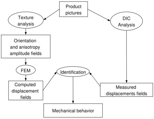
estimate displacement fields from various pictures of a specimen subjected to a mechanical loading. Last, an anisotropic elastic model is proposed, based on the determined orien-tation map. The latter is used to identify the unknown elastic moduli of the elementary representative volume, and to validate the identified parameters from a comparison between computed and measured displacement fields. A schematic of the different steps is presented in Figure 1. It will be followed herein.
Section II introduces the material under consideration, the crimping process and shows different types of crimped specimens. Section III presents briefly the local texture analysis and its results on a crimped specimen. Section IV gives the basics of the DIC procedure that allows one to obtain displacement fields decomposed over a continuous bilinear interpolation basis. A finite-element model of the anisotropic elastic solid behavior adopted herein is introduced in Section V. The key procedure of identification of the local anisotropic elastic properties is presented in Section VI, together with the results of the computed displacement
fields and their comparison with experimental compression test.
FIG. 1: Different steps of the image-based identification procedure.
II. CRIMPED GLASS WOOL
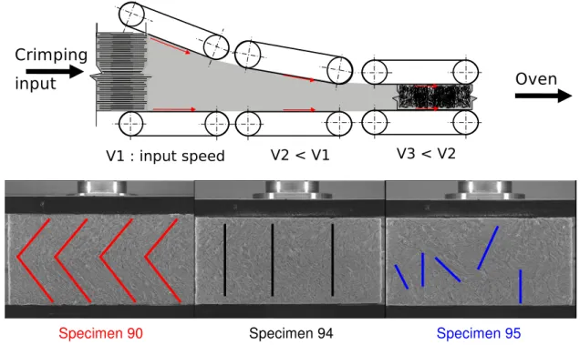
Glass wool is a cellular solid made of glass fibers with micrometric diameter and milli-metric to centimilli-metric length sprayed with a binder, and cured in an oven for freezing the arrangement of the fibers and hence providing some elasticity. To increase the mechanical performances, the fiber mat is processed before the curing stage to produce a structure en-dowing the material with a higher mechanical strength. This step is called crimping and it produces a better mechanical behavior due to a more favorable fiber orientation. However, the increase of stiffness goes together with an enhanced thermal conductivity, so that de-pending on applications, a compromise between mechanical and thermal properties has to be obtained. The crimping process shown schematically in Figure 2 (top) performs a com-pression of the fiber mat both across its thickness and along the line direction because of the progressive reduction of velocity of the conveyor belts in which the mat is introduced. A horizontal compression is taking place at each belt transition, which produces a “buckling”
or “folding” of the layers of higher fiber density. This process modifies significantly the fiber orientation as shown in Figure 2 (bottom). As a result, the elastic response of the finished product and its load bearing capacities are very sensitive to this crimping process. The aim of this study is to be able to predict the mechanical performances from a simple examination of its texture, i.e., a single picture prior to any mechanical load.
FIG. 2: Schematic view of the crimping process (top) and examples of crimped textures with characteristic features such as “V-shaped” crimping (left), fine-scale vertical texture (center), and coarse isotropic texture (right).
III. ANISOTROPY ANALYSIS
The detection of anisotropy of an element is performed by analyzing the change of gray levels in different directions, the direction where the variation is maximum is orthogonal to the principal axis of anisotropy. There are numerous methods using the gradient of gray level to capture changes in gray levels, which implicitly assume the image to be sufficiently smooth3,4 to use its gradients. The method used here does not require this smoothness
frequency modes)5
.
The analysis is based on the regularized correlation texture tensor of small sub-images extracted from a digital picture of the product face. Let f (x) be the gray-scale value of each pixel of the sub-image. The following tensor is computed from the discrete Fourier transform ˜f (k)
T= Z Z
| ˜f (k)|2k⊗ k
|k|2α dk (1)
For α = 0, the above tensor may be interpreted as the curvature tensor of the auto-correlation function at the origin. Its two orthogonal eigen-vectors provide the directions of highest and least persistence of the gray-levels and hence the anisotropy axis of the texture of the sub-image. For a non-smooth image, the curvature tensor of the auto-correlation does not exist, and hence a power-law filtering (factor |k|2α) is introduced to smoothen the auto-correlation
function and render the estimation less prone to pixel-scale noise. The parameter α may be evaluated a priori from the regularity of the analyzed image.
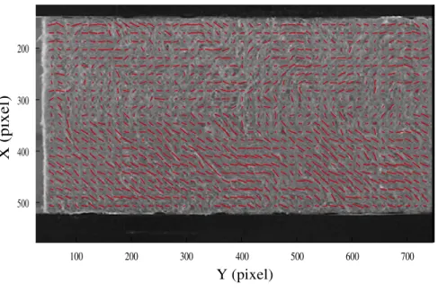
The deviatoric part of the tensor T gives an estimate of the amplitude of the anisotropy, in addition to the dominant orientation. Figure 3 shows an example of the extraction of the principal orientation map on a crimped structure (specimen 90) with a sub-image size equal to 32 × 32 pixels.
IV. DISPLACEMENT FIELD MEASUREMENT
The texture of the product after crimping is strongly heterogeneous, and hence the present analysis calls for a local characterization. For this purpose, a full field analysis of the displacement under different loadings is useful. A digital image correlation (DIC) technique6
is applied to a series of pictures taken at different stages of loading from a side view. The specificity of the latter is that it provides a continuous displacement field based on finite element shape functions (quadratic elements, polynomial shape functions of order 1 in both space directions). The technique allows one to obtain both a good spatial resolution (i.e., 16 × 16 pixels per element) and good displacement uncertainty (standard deviation typically of the order of a few 10−2 pixel).
Let f (x) and g(x) be a gray-scale representation of the images of a reference and deformed image respectively. The digital image correlation technique is based on the assumption of the passive evolution of the microstructure, so that the displacement field u(x) obeys the following optical flow conservation property
g(x) = f [x + u(x)] (2)
The ill-posed problem of determining the displacement field is first regularized by prescribing a restricted subspace for u, here chosen to be finite-element shape functions, Nn(x), of
quadratic elements with polynomials of order 1 in both space directions
uα(x) =
X
n
aαnNn(x) (3)
where α gives the direction x or y of the component of the displacement, and n labels the different shape functions. This basis will reveal convenient for the subsequent identification step, as exactly the same mesh will be used. Since the optical flow conservation cannot hold strictly pixel-wise, a weaker formulation is substituted (least squares minimization)
dn= Argmin Z Z g(x) − f [x +X n anNn(x)] !2 dx (4)
The non-linearity of Equation (4) is dealt with using a Newton linearization scheme on a series of low-pass filtered images down to the original (i.e., unfiltered) ones. Thus the solution is obtained iteratively from linear problems and deformed image corrections, until
best coincidence is achieved with the reference image. Each linear problem consists in solving [M ]{a} = {b} (5) where Mαnβm = Z Z [Nm(x)Nn(x)∂αf (x)∂βf (x)]dx (6) and bαn = Z Z [g(x) − f (x)] Nn(x)∂αf (x)dx (7)
The matrix [M ] is symmetric, positive (when the system is invertible) and sparse. These properties are exploited to solve the linear system efficiently.
V. MODELING
The crimping process only very mildly affects the medium perpendicularly to the line and thickness directions so that a two dimensional description is appropriate. In terms of mechanical description, the known correlation between strength and elastic stiffness is exploited. Thus, a simple elastic description is sought. Because of the microstructure of the material, a locally orthotropic elastic description is chosen. Therefore, locally, four elastic constants are introduced, namely, Snn, Snt, Stt and Suu where n is the direction
along the fiber and t is the transverse one. They are considered to be homogeneous within the medium, i.e., density fluctuations are ignored as they are severely dampened by the compression taking place in the crimping machine. However, the disordered orientation induced by crimping is taken into account. From the local texture analysis, the orientation field is known, and hence the elasticity tensor is rotated to be expressed in the laboratory frame.
The above description is performed at a well-defined scale since the orientation is based on a sub-image partition of the face view of the specimen. The solution to the elastic problem is thus performed by using a finite element method based on quadrangular bi-linear elements, whose size matches exactly the sub-images used in the texture analysis. Similarly, the DIC analysis is also based on the same mesh, with a consistent kinematic description (i.e., same shape functions). The boundary conditions used in the finite element simulations are prescribed from the measured displacement (i.e., Dirichlet conditions). As soon as the four elastic constants are chosen, the elastic problem is fully determined.
VI. IDENTIFICATION TECHNIQUE AND VALIDATION
Different techniques exist to identify elastic properties. A first class called virtual fields method uses special fields (i.e., virtual strain fields) to extract unknown elastic parame-ters. A linear system is obtained and solved to get the elastic unknowns7,8. A second
class of technique uses the constitutive law error associated with finite element updating to identify isotropic or anisotropic elastic properties9–11. Another route, the Equilibrium gap
method12,13, exploits the equilibrium conditions written at the nodes of a FE model where
the displacements are known (since measured). In the present case, the local properties will depend on the dominant orientation. Consequently finite element updating in its primary writing14 is preferred. Another reason is that the measured displacement field is directly
compatible with finite element simulations.
A. Finite Element Updating
Finite element updating determines the elastic constants so that the computed displace-ment field matches as well as possible the measured displacedisplace-ment field. The computed displacement field is obtained by solving
[K(Si)]{u0} = {0} (8)
for all the internal nodes, and {u0} imposed from the measured values on the boundaries. In
this expression, [K] is the global stiffness matrix that depends on the four elastic constants Si. Once a first estimate of the displacement field is computed, four additional “auxiliary”
fields, {ui}, i = 1, ..., 4 are computed that correspond to incremental variations of the
displacement field for a corresponding change in each of the elastic constants
[K(Si)]{ui} = −
∂[K] ∂Si
{u0} (9)
The difference between the measured {um} and computed {u0} displacement fields is then
projected onto the four influence fields through the minimization of
J = Z Z {um} − {u0} − X i γi{ui} !2 dx (10)
The components γi allow one to correct the elastic constants to new values Si0 such that
S0
The procedure is carried out iteratively down to convergence. The residual error field e(x) = ({um(x)} − {u0(x)})2/σ2, where σ2 is the variance of the measured displacement field, is
used to quantify the discrepancy density after identification.
B. Identification results
The identification procedure has been tested on both uniaxial compression and combined compression/shear tests. The results presented below have been obtained on a compression test of specimen 90. The global error in terms of displacements has reached a value less than 5.3%. The above procedure provides only relative values of the elastic constants. The global compression stiffness is finally estimated via
Kglobal =
hFyitop+ hFyibottom
2 (hUyitop− hUyibottom)
(12)
and matched to the experimentally determined value to rescale all constants. Table I gives the optimized elastic properties. One notes that there is an important difference between the stiffness along the fiber direction as compared to the transverse one. This is due to the strong alignment of fibers with few interconnections between them.
TABLE I: Identified local elastic properties of specimen 90 in uniaxial compression.
Snn Snt Stt Suu
(kPa) (kPa) (kPa) (kPa) Identified value 353 0 1.53 115
Figure 4 shows that a good agreement is obtained between measured and predicted dis-placement fields.
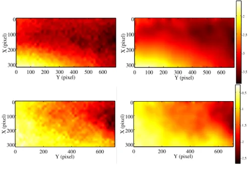
FIG. 4: Comparison between measured and identified displacement fields in pixels for specimen 90. The measured displacement field is shown on the left (vertical (top) and horizontal (bottom) components). The identified displacement fields are shown in the middle column, and the error fields are displayed on the right.
C. Validation
To test the predictive capacity of the previous approach, the displacement fields of a series of different specimens has been computed based on the previously determined elastic constants (i.e., from a compression test of specimen 90). Figures 5, 6, 7 show a direct comparison between measurements and predictions of both components of the displacement field for specimen 91, 94 and 95. The global error between predicted and measured fields is 4.1 % for specimen 91, 3.8 % for specimen 94, and 7 % for specimen 95.
FIG. 5: Comparison between measured (left) and computed (right) displacement fields in pixel relative to specimen 91 (vertical (top) and horizontal (bottom) displacement components).
FIG. 6: Comparison between measured (left) and computed (right) displacement fields in pixel relative to specimen 94 (vertical (top) and horizontal (bottom) displacement components).
FIG. 7: Comparison between measured (left) and computed (right) displacement fields in pixel relative to specimen 95 (vertical (top) and horizontal (bottom) displacement components).
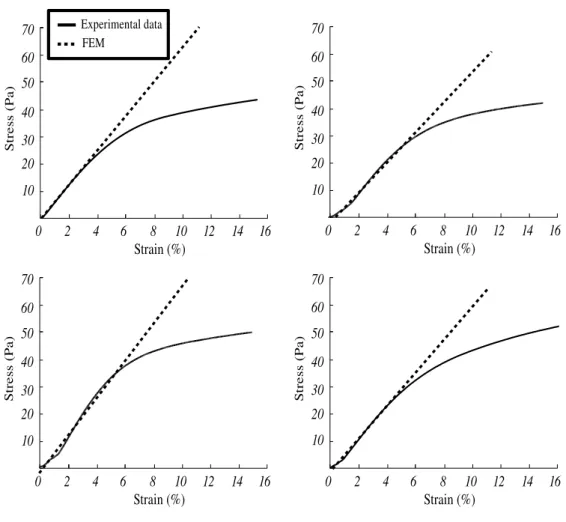
The quality of the identification is further tested by computing the expected stiffness and comparing it to the experimental stress-strain curves as shown in Figure 8 for the different crimped specimens studied in the previous section. (Note that very small strain levels (< 1%) are unreliable because of initial contact imperfections.) This validates the identified anisotropic elastic constants of specimen 90 that are given in Table I.
FIG. 8: Experimental stress-strain compression data for specimen 90 (top, left), specimen 91 (top, right), specimen 94 (bottom, left), specimen 95 (bottom, right). The computed elastic stiffness is shown as a dashed line in each plot.
D. Comparison with a global approach
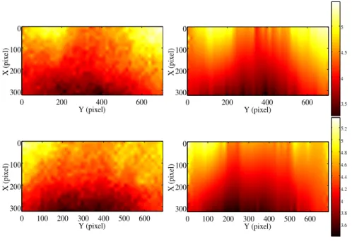
The usefulness of the present approach is twofold: first, it is important to perform the identification at a local scale in order to be able to predict the effect of the ‘microstruc-ture’ (i.e. local orientation of the texture) on the global properties. Second, the value of the analysis should be gauged as compared to the prediction performance of a mechanical description where the texture would be ignored. To answer this second question, it is pro-posed to compare the present identification procedure to that obtained with the assumption of homogeneity of the elastic parameters. This comparison is performed on the example
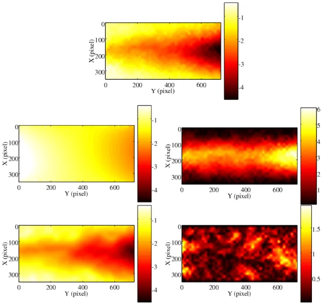
shown in Figure 3. The results are presented in Figure 9 where the horizontal component of the displacement is displayed for the experimental case, the globally homogeneous elastic description, and the locally homogeneous description. The error maps (right part of Fig-ure 9) and the global error for the globally homogeneous elastic description is close to 18 % compared with the 5.3 % shown in Section VI B. The global error is divided by three. This result shows the significant advantage of the proposed methodology.
FIG. 9: Top: measured horizontal field. Middle left: computed horizontal displacement field using globally homogeneous elastic moduli. Middle right: associated error field. Bottom left: computed horizontal displacement field using locally homogeneous parameters. Bottom right: associated error map.
VII. CONCLUSION
This study presents a global identification procedure for mechanical properties of glass wool based on different quantitative image analyses. From an experimentally observed texture of a heterogeneous material, it allows one to have access to the local elastic properties. Being based on full field measurements, it allows for a full benefit of the rich amount of data and not only global macroscopic measurements.
The complete procedure (i.e., mechanical test with image acquisition, analysis of the displacement field by digital image correlation, texture analysis and identification), has been followed up to the quantification of the elastic constants. The assumed homogeneity of the elastic properties and determined local orientations are thereby essentially validated from the good reproduction of the experimental displacement field on one specimen.
The potential of this procedure as a kind of “virtual testing” has been highlighted by computing ex ante estimates of the displacement fields of other specimens using the same elastic constants. Those displacement fields and stiffness estimates compare quite accurately with ex post experimentally determined values.
∗ Electronic address: [email protected]
† Electronic address: [email protected] ‡ Electronic address: [email protected]
§ Electronic address: [email protected]
1 S. Bergonnier, F. Hild, S. Roux, Local anisotropy analysis for non-smooth images, Patt. Recogn. 40 (2007) 544-556.
2 P.K. Rastogi, eds., Photomechanics, Springer, Berlin (Germany), (2000).
3 A. Rao, A Taxonomy for Texture Description and Identification, Springer, Berlin (Germany), 1990.
application to texture characterization, Signal Processing 83 (2003) 14871503.
5 S. Bergonnier, F. Hild, S. Roux, Strain heterogeneities and local anisotropy in crimped glass wool, J. Mat. Sci. 40 (2005) 5949-59-54.
6 G. Besnard, F. Hild, S. Roux, “Finite-element” displacement fields analysis from digital images: Application to Portevin-Le Chˆatelier bands, Exp. Mech. 46 (2006) 789-803.
7 M. Gr´ediac, Principe des travaux virtuels et identification, C. R. Acad Sci. Paris 309 (1989) 1-5.
8 M. Gr´ediac, The use of full-field measurement methods in composite material characterization: interest and limitations, Composites: Part A 35 (2004) 751-761.
9 R.V. Kohn, B.D. Lowe, A Variational Method for Parameter Identification, Math. Mod. Num. Ana. 22 (1988) 119-158.
10 P. Ladev`eze, D. Nedjar, M. Reynier, Updating of Finite Element Models Using Vibration Tests, AIAA 32 (1994) 1485-1491.
11 G. Geymonat, F. Hild, S. Pagano, Identification of elastic parameters by displacement field measurement, C. R. Mecanique 330 (2002) 403-408.
12 D. Claire, F. Hild, S. Roux, Identification of damage fields using kinematic measurements, C. R. Mecanique 330 (2002) 729-734.
13 D. Claire, F. Hild, S. Roux, A finite element formulation to identify damage fields: The equilibrium gap method, Int. J. Num. Meth. Engng. 61 (2004) 189-208.
14 K.T. Kavanagh, R.W. Clough, Finite Element Applications in the Characterization of Elastic Solids, Int. J. Solids Struct. 7 (1971) 11-23.