A mean field theory for diffusion in a dilute multi-component alloy: a new model for the effect of solutes on self-diffusion

HAL Id: hal-00513556

https://hal.archives-ouvertes.fr/hal-00513556

Submitted on 1 Sep 2010

solutes on self-diffusion

Maylise Nastar

To cite this version:

Maylise Nastar. A mean field theory for diffusion in a dilute multi-component alloy: a new model for the effect of solutes on self-diffusion. Philosophical Magazine, Taylor & Francis, 2005, 85 (32), pp.3767-3794. �10.1080/14786430500228390�. �hal-00513556�

For Peer Review Only

A mean field theory for diffusion in a dilute multi-component alloy: a new model for the effect of solutes on

self-diffusion

Journal: Philosophical Magazine & Philosophical Magazine Letters Manuscript ID: TPHM-04-Dec-0137.R1

Journal Selection: Philosophical Magazine Date Submitted by the

Author: 30-May-2005

Complete List of Authors: Nastar, Maylise; CEA-Saclay, DMN/SRMP

Keywords:

transport properties, statistical physics, non-equilibrium

phenomena, metallic alloys, diffusion, atomistic simulation, atomic transport, atomic defects

Keywords (user supplied):

For Peer Review Only

A mean field theory for diffusion in a dilute multi-component alloy : a new model for the effect of solutes on self-diffusion

Maylise Nastar∗

Service de Recherches de M´etallurgie Physique, CEA/Saclay, 91191 Gif-sur-Yvette, France.

(Dated: May 30, 2005)

ABSTRACT

A new extension of the self-consistent mean field (SCMF) theory is developed to describe diffusion in dilute alloys, special attention being paid to the problem of self-diffusion in presence of solute atoms. We start from a microscopic model of the atom-vacancy exchange frequency including nearest neighbour interactions and derive kinetic equations from a Master equation. The non-equilibrium dis-tribution function is expressed trough time dependent effective interactions. Their range of interaction is controlling the level of description of the paths of a vacancy after a first exchange. In contrast to the previous diffusion models devoted to concentrated alloys, the present formulation makes appear into the final result several exchange frequencies associated to a given atom depending on the chemical species of the atoms nearby. A first approximation restricted to nearest neighbour effective interactions yields analytical expressions of the transport coefficients of a face centered cubic dilute binary alloy. ∗

Electronic address: [email protected]

1 2 3 4 5 6 7 8 9 10 11 12 13 14 15 16 17 18 19 20 21 22 23 24 25 26 27 28 29 30 31 32 33 34 35 36 37 38 39 40 41 42 43 44 45 46 47 48 49 50 51

For Peer Review Only

The phenomenological coefficients are equivalent to the ones obtained using the five frequency model within the first shell approximation. A new expression of the self-diffusion coefficient is proposed and compared to Monte carlo (MC) simulations using the same atomic diffusion model. The SCMF theory reproduces the main tendencies of the MC simulations, in particular within the random alloy region where the recent five-frequency model was not satisfying. The limitations and future improvements of the SCMF approach are easily related to the range of the effective interactions considered.

I. INTRODUCTION

Matter transport in alloys is generally controlled by microscopic jumps of point defects. In the limiting case of a very dilute binary alloy, the link between these microscopic jump frequencies and the phe-nomenological transport coefficients Lij has been established for the main crystallographic structures (Allnatt and Lidiard 1993). In that case it is possible after an exchange of a vacancy with a given atom to account for all the different vacancy paths and determine the probability for a vacancy to exchange again with the same atom. The five-frequency model for a dilute face centered cubic (fcc) alloy is a well-known example of this kind (Howard and Lidiard 1963, 1964 and Allnatt 1981 for the exact solution). But as soon as we consider the effect of adding a third atomic species or increas-ing the amount of solutes rigorous models are lackincreas-ing. We present here the example of estimation of the diffusion coefficient of an isotope A∗ in a binary alloy AB (solute B in A) which remains a challenge. Even so the question is of a great practical interest since many experimental results are measurements of isotope diffusion coefficients. Within a multi-frequency model, the isotope diffusion coefficient, DA∗, is a sum of several partial diffusion coefficients relative to the position of A∗ with 1 2 3 4 5 6 7 8 9 10 11 12 13 14 15 16 17 18 19 20 21 22 23 24 25 26 27 28 29 30 31 32 33 34 35 36 37 38 39 40 41 42 43 44 45 46 47 48 49 50 51

For Peer Review Only

respect to the solute B for which the vacancy paths are performed within a cut-off radius. Following the approach of Howard and Manning (1967), Ishioka and Koiwa (1984) performed a more extensive calculation based on larger cut-off radius but some of their results were called into question from 1986 (Allnatt and Lidiard 1986). For example Allnatt and Lidiard (1986) have pointed out that DA∗ should decrease with the B solute concentration when the vacancy-solute exchange frequency is zero since then an addition of immobile solute atoms should slow down the diffusion of tracer solvent atoms A∗. A recent publication suggested a possible reason for these shortcomings by showing that the correlation effects between different vacancy encounters were not introduced properly (Szab´o and Beke 2004). An alternative theoretical approach which was first developed to treat diffusion in concentrated alloys (Manning 1971, Moleko, Allnatt and Allnatt 1989, Nas-tar et al. 2000) was verified to be more reliable for the prediction of diffusion of isotope A∗ in the limiting case of a ’random dilute alloy’ AB. In a ’random alloy’ first introduced by Manning (1971) a vacancy-atom exchange frequency, ωx is taken to be characteristic of the atom x but independent of the environment which implies no interaction between the atoms. Among the random lattice gas models, the predictions of Moleko, Allnatt and Allnatt (1989) were shown to be very close to recent Monte Carlo simulations (Belova and Murch 2003b).

In a fcc alloy with interactions, recent Monte Carlo simulations (Belova and Murch 2003a) have shown that both treatments of Howard and Manning (1967) and Ishioka and Koiwa (1984) have major shortcomings in describing self-diffusion in presence of solute atoms. There are very few alternatives to these multi-frequency models. A mean field approach like the Path Probability Method (PPM) is based on an atomic diffusion model which depends on the local environment (Sato and Kikuchi 1 2 3 4 5 6 7 8 9 10 11 12 13 14 15 16 17 18 19 20 21 22 23 24 25 26 27 28 29 30 31 32 33 34 35 36 37 38 39 40 41 42 43 44 45 46 47 48 49 50 51

For Peer Review Only

1983, Sato et al. 1985 correcting the first versions of Kikuchi and Sato 1969). But the statistical approximation used to average the matter flow under a gradient of chemical potential and formulate the Lij leads to averaged jump frequencies, each one representing an atomic species. A recent approach based on the same jump frequency model and starting from a Taylor series expansion in powers of time of the time correlation functions appearing in the Lij (Qin et al. 1998) employs the detailed balance principle to making appear a set of jump frequencies associated to a given chemical species. However, the latter principle is not sufficient to make appear rotational jumps of type ω1 from other jumps like the dissociative jump of type ω3 in a fcc alloy. Indeed both jump frequencies describe a jump leaving the same initial state and they differ by their saddle point position only so that they cannot be connected by a detailed balance equality. The empirical approach of Bakker and Stolwijk (Bakker 1979, Stolwijk 1981) also based on an averaged treatment of the jump frequencies leads to the same conclusions. Our previous work based on a SCMF theory yielded a full Onsager matrix from an atomic diffusion model (Nastar 2000) but the resulting Lij made appear a limited number of averaged jump frequencies too. A severe consequence is that non-diagonal phenomenological coefficients are automatically positive which means that for example a kinetic coupling inducing an inversion of the direction of an atomic flux would not be predicted by such models. Our purpose is to show that within a self-consistent mean field (SCMF) formalism one can make appear a set of jump frequencies which in the particular case of a dilute alloy is equivalent to the one defined by a multi-frequency model. The example of diffusion in a fcc binary dilute alloy (solute B in A) with first nearest neighbour interactions will be treated. It requires that at least five jump frequencies comes out of the present approach : the B-vacancy exchange frequency (ω2) and the 1 2 3 4 5 6 7 8 9 10 11 12 13 14 15 16 17 18 19 20 21 22 23 24 25 26 27 28 29 30 31 32 33 34 35 36 37 38 39 40 41 42 43 44 45 46 47 48 49 50 51

For Peer Review Only

four different A-vacancy exchange frequencies : ω3 when B is nearest neighbour of vacancy, ω4 the reverse jump of ω3, ω1 when B is nearest neighbour of both species of the exchanging pair and ω0 for the other jumps (Howard and Lidiard 1963, 1964, Allnatt and Lidiard 1993). First objective will be to recover the formulae of the Lij of the five-frequency models and then to propose a new analytical model of the self-diffusion coefficient to first order in solute concentration. To check the validity of the later result, we perform Monte Carlo simulations based on the same atomic diffusion model with nearest neighbour interactions. We use a slightly different procedure than the one of Belova and Murch (2003a) : the atomic diffusion model is defined everywhere so that the present MC simulations do not prevent configurations in which solute atoms are in close proximity.

First section starts from an atomic diffusion model and derives kinetic equations by means of a master equation. Non-equilibrium averages are estimated using a non-equilibrium distribution function which is defined in terms of a time dependent effective hamiltonian. In the following sections the SCMF approach is applied to fcc alloys. Section III writes the kinetic equations for a f cc alloy in the case of an effective hamiltonian restricted to nearest neighbour (nn) interactions and yields an analytical expression of the transport coefficients in the limit of a dilute alloy. The present theory is compared to the five-frequency models (Allnatt and Lidiard 1993). The extension to multi-component alloys being quite obvious, a new formulae is suggested for the tracer diffusion DA∗ in AB. Section IV presents the atomic diffusion models and the conditions of MC simulations. Section V is a discussion of the results compared to the MC simulations and the previous models, first in the random alloy limit and second in alloys with interactions.

1 2 3 4 5 6 7 8 9 10 11 12 13 14 15 16 17 18 19 20 21 22 23 24 25 26 27 28 29 30 31 32 33 34 35 36 37 38 39 40 41 42 43 44 45 46 47 48 49 50 51

For Peer Review Only

II. THE SCMF THEORY

Within the theory of linear non-equilibrium thermodynamics, the Lij are defined as the constants coupling the fluxes to the external forces which will be here the gradients of chemical potentials. The evaluation of ensemble averages of a system subject to an external gradient of chemical potential requires to define a non-equilibrium distribution function. First part of this chapter provides with a general formulae of the non-equilibrium distribution function in terms of non-equilibrium effective interactions. We introduce then a Master Equation which expresses the fact that transitions between a given configuration and the others are controlled by the vacancy jump frequencies. We obtain then a series of kinetic equations which describe the time evolution of mean occupancies of resp. one chemical species on one site, two chemical species on a pair of sites, etc.. The Lij are identified from the fluxes which are deduced from the continuity equation applied to the time derivative of point averages. As a first approximation we assume the effective Hamiltonian contains pair effective interactions only. We deduce their expressions as a function of gradients of chemical potentials by applying the steady state conditions to the time derivative of the two-point averages. The resulting Lij are written as a function of equilibrium averages. Last part of the section is demonstrating that the Onsager reciprocal relation is verified.

A. The non-equilibrium distribution function

The alloy is represented by a system of interacting atoms and vacancies distributed on a rigid lattice. A configuration of the alloy is defined by a vector n, the components of which are the occupation 1 2 3 4 5 6 7 8 9 10 11 12 13 14 15 16 17 18 19 20 21 22 23 24 25 26 27 28 29 30 31 32 33 34 35 36 37 38 39 40 41 42 43 44 45 46 47 48 49 50 51

For Peer Review Only

numbers of all species on all sites {nA₁, nB₁, . . . , nv₁; n₂A, nB₂, . . . , nv₂; . . .} such that na_i = 1 if site is occupied by species a and zero if else. The corresponding configurational Hamiltonian is noted H.b

Transitions between the different configurations of the system are controlled by exchanges between atoms and vacancies. The probability per time unit of a single jump of an atom α at a site i into a vacancy v at a site j is noted w_bαv

ij (n).

Changes of a configuration n are specified by the master equation, dP (n, t)b dt = X ˜ n h c W (˜n → n)P (˜b n, t) −W (n → ˜c n)P (n, t)b i , (1)

where W (n → ˜c n) is the transition probability from a configuration n to a configuration ˜n per time

unit : it is defined in terms of the microscopic frequencies controlling the diffusion of atoms. By construction of the microscopic jump frequencies which obey micro-reversibility, each term of the sum entering equation (1) is zero when P is taken as the equilibrium distribution functionb Pb₀ :

b P0(n) = exp[β(Ω0+ X α µα X i nα_i −H)].b (2)

Here β = 1/T is the reciprocal temperature, Ω is the grand canonical potential found from the usual normalization condition P

nPb₀(n) = 1, and µ_α is the chemical potential of the atoms α relative to

vacancies, i.e. the difference between the chemical potential of atoms α and of vacancies. Indeed, since we describe a system with a fixed number of sites Ns, the constraint on site i,Panai = 1, implies that there are only (Nc− 1) independent chemical potentials, where Nc is the number of components in a many-component system ; for our convenience we choose chemical potentials of atoms relative to vacancy as independent ones.

[∗] We mark functions depending on configuration by the ‘hat’ sign, e.g. H stands forb H(n).b

1 2 3 4 5 6 7 8 9 10 11 12 13 14 15 16 17 18 19 20 21 22 23 24 25 26 27 28 29 30 31 32 33 34 35 36 37 38 39 40 41 42 43 44 45 46 47 48 49 50 51

For Peer Review Only

Following Vaks (1996), the non-equilibrium distribution function entering equation (1) is expressed in terms of a time dependent effective hamiltonian bh(t) :

b

P (n, t) =Pb₀(n)Pb₁(n, t), (3)

where Pb₀(n) is the equilibrium distribution function and Pb₁(n, t) = exp{β[δΩ(t) +P_α,iδµα_i(t)nα_i − b

h(t)]} is the non equilibrium contribution which is equal to one at equilibrium. The time-dependent effective Hamiltonian is written as a polynomial function of the occupation numbers

b h(t) = 1 2! X αβ,i6=j v(2)αβ_ij (t)nα_inβ_j + 1 3! X αβγ,i6=j6=k v(3)αβγ_ijk (t)nα_inβ_jnγ_k+ . . . , (4)

where v(N )αβ..._ij... (t) are time dependent N -body effective interactions, which are unknown and must be obtained solving the master equation. In fact, instead of searchingP (n, t) as a solution of the masterb

equation (1) we defineP by its moments, hnb α_ii, hnα_inβ_ji, . . . , which we later call the one, two, ..., point

averages, and establish the kinetic equations for the latter. Furthermore the non-equilibrium averages appearing in the kinetic equations are split up into two parts : a non-equilibrium contribution denoted by Pb₁ which is considered as a function to be averaged and the equilibrium average which is seen as

the distribution function to be employed to calculating the ensemble average. It is convenient in doing so because the new averages to be calculated can now be connected to the well known thermodynamic statistical approximations. Two hierarchies of approximations come up at this point. First hierarchy is related to the statistical approximation used to calculate the equilibrium averages. The second level of approximation is associated with the number of unknown effective interactions of the time

[†] Referred to the ”cluster expansion theorem” (Sanchez 1984), any quantity which is a function of configuration only can be written in the form of equation (4)

1 2 3 4 5 6 7 8 9 10 11 12 13 14 15 16 17 18 19 20 21 22 23 24 25 26 27 28 29 30 31 32 33 34 35 36 37 38 39 40 41 42 43 44 45 46 47 48 49 50 51

For Peer Review Only

dependent effective Hamiltonian that we consider. It determines the number of independent kinetic equations. For example truncation of the effective Hamiltonian after the pair effective interactions limits the system of independent kinetic equations to the point and two-point equations and the stationarity conditions are not guaranteed to be satisfied by the N-point kinetic equations (N > 2). Self-consistency is then guaranteed up to the two-point averages.

B. Kinetic equations

Starting from the master equation, the time derivative of such averages simply writes (demonstration is given in Appendix A of Nastar 2000),

dhnα_inβ_jnγ_k. . .i dt = X s6=i6=j6=... hnβ_jnγ_k. . . [nα_snv_iwb αv si − nαinvswb αv is ]i + X s6=i6=j6=... hnα_inγ_k. . . [nβ_snv_jwb βv sj − n β jn v swb βv js]i + . . . , (5) where the brackets indicate non-equilibrium ensemble averages. To calculate such averages we use two approximations : first we restrict the effective Hamiltonian to pair effective interactions, second we use a better statistical approximation than the Bragg Williams approximation used in (Nastar 2000). The complete procedure is presented below for a general model of alloy where the equilibrium averages are not explicitly calculated. Chapter (III) applies the model to an fcc dilute alloy and provides with a complete calculation of the Lij and the tracer correlation factor of a binary alloy.

After linearization with respect to the terms of the form β(δµα

s − δµαi) and βbhα_s together with the

principle of detailed balance, we obtain for the 2-point average (details are given in appendix A) : dhnα_inβ_ji dt = β X s6=i6=j6=... hnβ_j[nα_snv_iωb αv si (δµαs − δµαi −hbα_s +bhα_i)]i(0)+ 1 2 3 4 5 6 7 8 9 10 11 12 13 14 15 16 17 18 19 20 21 22 23 24 25 26 27 28 29 30 31 32 33 34 35 36 37 38 39 40 41 42 43 44 45 46 47 48 49 50 51

For Peer Review Only

β X s6=i6=j6=... hnα_i[nβ_snv_jωb βv sj(δµ β s − δµ β j −bhβ_s +bhβ_j)]i(0), (6)

where(0)means averaging over the equilibrium distribution function P(0), andbhα_s is the partial

deriva-tive ofbh with respect to nα_s.(δµβ_s− δµβ_j) is equivalent to the difference of the total chemical potentials

since the equilibrium contribution to the difference is equal to zero.

Flux of atomic species is deduced from the continuity equation applied to the kinetic equation of the one-point average : dhnα_ii dt = − X s6=i J_i→sα , (7) and is recognized to be : J_i→sα = −β[hnα_inv_sωb αv is (µαs − µαi −bhα_s +bhα_i)i(0). (8)

Following the same procedure presented in (Nastar 2000), we could show that close to an homogeneous equilibrium and under an homogeneous gradient of chemical potential, flux Jα

i→j and dhnα_inβ_ji dt − dhnα jn β ii dt depends on asymmetrical effective interactions of type (v_ijαβ− vαβ_ji ). An easy way to account for this property is to put equal to zero the symmetric part of the effective interactions and assume v_ijαβ = −v_jiαβ and vαα

ij = 0. In an isotope crystal, the diffusion problem is mono-dimensional : we choose an axis along which the atomic fluxes are estimated. This axis is an axis of rotational symmetry so that we group rotationally equivalent sites together. Furthermore, in an homogeneous equilibrium state, the local concentrations do not depend on sites : cα_i = cα, where cα is the composition of atoms α. For such conditions the system of equations has translational symmetry ; nothing is changed under the transformation r → r + R (where R is a vector between two arbitrary sites of the lattice). The solution may be taken with the same symmetry : v_ijαβ = vαβ(ri+R, rj+R). Therefore, the asymmetrical 1 2 3 4 5 6 7 8 9 10 11 12 13 14 15 16 17 18 19 20 21 22 23 24 25 26 27 28 29 30 31 32 33 34 35 36 37 38 39 40 41 42 43 44 45 46 47 48 49 50 51

For Peer Review Only

property added to the translation property reduce the number of unknown effective interactions to the number of non-equivalent two-point averages to be considered. Each non-equivalent pair of points is labelled by a number iv (iv = 1 for the first nearest neighbour two-point average) and is associated to a positive effective asymmetrical interaction : v_(ασ)iv = vασ_(ii+₎iv in which (ii+)iv is the axis coordinate of the vector linking both sites.

The antisymmetric property of v leads to a simplification of the flux :

J_i→iα + = −β[hnα_inv_i+ω_biiαv+(µα_i+ − µα_i + 2hα_i)i(0). (9)

Since the effective Hamiltonian contains pair interactions only we write down the flux in terms of the v(ασ)iv : J_i→iα + = −βl(0)_α (µα_i+ − µα_i) − β X σ,iv [lα(σ, iv)v(ασ)iv], (10) with l(0)_α = γ_(ii+₎1hnα_inv_i+ωb αv ii+i(0) (11) and lα(σ, iv) = 2 X p6=i6=i+_,σ γ_(ii+₎1γ_(ip)ivhnα_inv_i+nσ_pωb αv ii+i (0) v ασ ip viv (ασ) . (12)

γ_(ip)iv is equal to 1 if sites i and p form a pair of type i_v and is equal to 0 if else.

The phenomenological coefficients are by definition the coefficients which relate fluxes to thermody-namic forces (here gradients of chemical potentials). They have the form :

1/βLαα= lα(0)(α) + X σ,iv lα(σ, iv)v(ασ)iv(α), (13) 1 2 3 4 5 6 7 8 9 10 11 12 13 14 15 16 17 18 19 20 21 22 23 24 25 26 27 28 29 30 31 32 33 34 35 36 37 38 39 40 41 42 43 44 45 46 47 48 49 50 51

For Peer Review Only

1/βLαβ =

X

σ,iv

lα(σ, iv)v(ασ)iv(β), (14)

where v_(αβ)iv(σ) is the σ coordinate of v_(αβ)iv : v_(αβ)iv = P_σv_(αβ)iv(σ)(∇µ_σ), with (∇µ_σ) = γ(ii+₎1(µσ_i+ − µσ_i). In setting down equation (10) we have omitted the time dependence of v since the kinetic equations will be solved under steady state conditions. The two point kinetic equations alone are required for the estimation of v. They can be written as :

1/βdhn α in β ji(iv) dt = mα(β, iv)∇µα− mβ(α, iv)∇µβ +X jv [t_(αβ)iv_,(αβ)jvv_(αβ)jv + X γ t_(αβ)iv_,(αγ)jvv_(αγ)jv + X γ t_(αβ)iv_,(γβ)jvv_(γβ)jv] (15) with mσ(α, iv) = X s6=i6=i+ γ_(ii+₎ivγ_(is)1hn_iσ+nα_snv_iωb σv sii(0)(µσs − µσi)/∇µσ, (16) t_(αβ)iv_,(ασ)jv = [ X s6=i6=i+ γ_(ii+₎ivγ_(is)1hnβ i+nα_snv_iωb αv si ( X p6=j,s γ_(ip)jvvασ_ip nσ_p − X p6=i,i+ γ_(sp)jvvασ_spnσ_p)i(0)]/v_(ασ)jv(17), and t_(αβ)iv_,(αβ)jv = t_(αβ)iv_,(ασ)jv(σ ≡ β) + t_(αβ)iv_,(σβ)jv(σ ≡ α) +[γ_(ij)iv X s6=i6=j γ_(is)1hnβ_jnα_snv_iω_bαv_si (γ_(ij)jvv_ijαβ− γ_(sj)jvv_sjαβ)i +γ_(ij)iv X s6=i6=j γ_(js)1hnα_in_sβnv_jω_bsjβv(γ_(ij)jvv_ijαβ− γ_(si)jvvβα_si )i(0)]/v_(αβ)jv. (18) .

We note the symmetry : t_(αβ)iv_,(ασ)jv = −t_(αβ)iv_,(σα)jv and t_(βα)iv_,(σα)jv = t_(αβ)iv_,(ασ)jv. 1 2 3 4 5 6 7 8 9 10 11 12 13 14 15 16 17 18 19 20 21 22 23 24 25 26 27 28 29 30 31 32 33 34 35 36 37 38 39 40 41 42 43 44 45 46 47 48 49 50 51

For Peer Review Only

The unknown effective interactions are then solution of equation (15) under steady state conditions (derivatives with time are equal to zero). They are given as a linear combination of the gradients of chemical potential :

¯¯

T ¯v = ¯b, (19)

Components of ¯b and ¯v, b(i) and v(i), are associated to the couple (α, σ)iv _{with i = (N}

esp∗ (Nesp+ 1)/2) ∗ (iv − 1) + Nesp(α − 1) + σ. b(i) is equal to −mα(σ, iv)∇µα+ mσ(α, iv)∇µσ. Element t(i, j) of matrix T is associated to the couple ((ασ)iv, (βγ)jv) such that i is the index defined above and j = (Nesp∗ (Nesp+ 1)/2) ∗ (jv− 1) + Nesp(β − 1) + γ.

C. The Onsager reciprocal relation

The SCMF approximation limited to nn effective interactions is shown to satisfy the Onsager reciprocal relation, that is, Lαβ = Lβα.

For that it is sufficient to note that

lα(σ, 1) = 2mα(σ, 1). (20)

Using this relationship we deduce Lαβ from equation (14) where the unknown v(ασ)1(β) are calculated using the system of equations (15) :

Lαβ = +2 X σ>α mα(σ, 1)t−1_(ασ)1_(αβ)1mβ(α, 1) +2X σ>β mα(σ, 1)t−1_(ασ)1_(βσ)1mβ(σ, 1) +2X σ>β mα(β, 1)t−1_(αβ)1_(βσ)1mβ(σ, 1), (21) 1 2 3 4 5 6 7 8 9 10 11 12 13 14 15 16 17 18 19 20 21 22 23 24 25 26 27 28 29 30 31 32 33 34 35 36 37 38 39 40 41 42 43 44 45 46 47 48 49 50 51

For Peer Review Only

where t−1_(ασ)1_(αβ)1 is the element of the inverse T matrix located at the arrow associated to (ασ)1 and the column associated to (αβ)1_{. In the same way, L}

βα is deduced from equation (14) by exchanging α and β where the unknown v_(βα)1(α) are calculated using the system of equations (15) :

Lβα= +2 X σ>β mβ(σ, 1)t−1_(βσ)1_(αβ)1mα(β, 1) +2X σ>α mβ(α, 1)t−1_(αβ)1_(ασ)1mα(σ, 1) +2X σ>β mβ(σ, 1)t−1_(βσ)1_(ασ)1mα(σ, 1)]; (22)

which leads to the equality : Lβα= Lαβ.

III. RESULTS

A. The fcc alloy

The preceding section has been concerned with the general expression of the Lij. To complete the derivation, the crystallographic structure needs to be specified. Indeed an explicit expression of the sums over neighbouring sites entering equations (16,17,18) will depend on the crystal. In the following sections we will illustrate the theory on the fcc crystallographic structure. Moreover, for the sake of simplicity and in order to keep analytical results, we make the approximation that the effective Hamiltonian is restricted to nearest neighbour (nn) interactions. Most of this section takes advantage of the homogeneity of the equilibrium state. In the dilute limit, one can show that N-point averages are equal to the product of point averages multiplied by an exponential of a binding energy so that they are characterized by their interacting bonds only and disconnected from the sites surrounding the N-point cluster. In the particular case of an Hamiltonian limited to nn interactions, the N-point 1 2 3 4 5 6 7 8 9 10 11 12 13 14 15 16 17 18 19 20 21 22 23 24 25 26 27 28 29 30 31 32 33 34 35 36 37 38 39 40 41 42 43 44 45 46 47 48 49 50 51

For Peer Review Only

averages are characterized by their nn pairs only. It is no more valid in concentrated alloys but we will make this assumption from the beginning since the kinetic equations will be later used in a fcc dilute alloy. There are two steps in the derivation. First step is to identify the N-point averages to be calculated and last step is to calculate them. Sums over neighbours entering the kinetic equations are calculated along a [100] symmetry axis. In practice, l(0)α of equation (11) may be written as

l(0)_α = γ(αv)1hn_αn_vω_bαvi(0), (23)

where indices entering equation (11) are eliminated since equilibrium averages are characterized by their first nearest neighbour bonds only and γ_(αv)1 function is introduced to notify that species α and v occupy nn sites. In the same way equation (16) reduces to :

mσ(α, 1) = −3γ(σv)1γ_(ασ)1hn_αn_σn_vω_bσvi(0)+ 2γ_(αv)1γ_(ασ)1γ_(σv)1hn_αn_σn_vw_bσvi(0), (24)

where summations over neighbours entering equation (16) are performed along the [100] axis.

We start with a pair of sites (ii+)1 located at the respective positions i and i + 1 along the [100] axis. Among the nn of i, there is one site at position (i + 1) which does not coincide with i+ and is not nn of i+ and there are four sites at position (i − 1) which are not nn of i+, which leads to the factor (1 − 4 = −3) in front of the first average of equation (24). Furthermore there are two sites at position (i + 1) which are nn of both s and i which explains the factor (2) in front of the second average. Since nn neighbour effective interactions are considered only, terms of type t_(αβ)1_,(αγ)1 are to retain only. They involve the calculation of four-point averages. The counting of these sums in a fcc crystal is presented in appendix B. 1 2 3 4 5 6 7 8 9 10 11 12 13 14 15 16 17 18 19 20 21 22 23 24 25 26 27 28 29 30 31 32 33 34 35 36 37 38 39 40 41 42 43 44 45 46 47 48 49 50 51

For Peer Review Only

t_(αβ)1_,(ασ)1 = −8γ_(αβ)1γ_(αv)1γ_(ασ)1hω_bαvn_αn_βn_vn_σi(0) −10γ_(αβ)1γ_(αv)1γ_(ασ)1γ_(σv)1hω_bαvn_αn_βn_vn_σi(0) +10γ_(αβ)1γ_(αv)1γ_(ασ)1γ_(σβ)1hω_bαvn_αn_βn_vn_σi(0)+ 11γ_(αβ)1γ_(αv)1γ_(σv)1hω_bαvn_αn_βn_vn_σi(0) −2γ_(αβ)1γ_(αv)1γ_(σv)1γ_(βσ)1hω_bαvn_αn_βn_vn_σi(0)− 2γ_(αβ)1γ_(αv)1γ_(σv)1γ_(βσ)1γ_(ασ)1hω_bαvn_αn_βn_vn_σi(0) −10γ_(αβ)1γ_(αv)1γ_(βv)1γ_(ασ)1hω_bαvn_αn_βn_vn_σi(0)+ 4γ_(αβ)1γ_(αv)1γ_(βv)1γ_(ασ)1γ_(σv)1hω_bαvn_αn_βn_vn_σi(0) +4γ(αβ)1γ_(αv)1γ_(βv)1γ_(ασ)1γ_(βσ)1hω_bαvn_αn_βn_vn_σi(0) +2γ(αβ)1γ_(αv)1γ_(βv)1γ_(ασ)1γ_(βσ)1γ_(σv)1hω_bαvn_αn_βn_vn_σi(0) −6γ_(αβ)1γ_(αv)1γ_(βv)1γ_(βσ)1γ_(σv)1hω_bαvn_αn_βn_vn_σi(0). (25) for t_(αβ)1_,(αβ)1 : t_(αβ)1_,(αβ)1 = t_(αβ)1_,(ασ)1(σ ≡ β) + t_(βα)1_,(βσ)1(σ ≡ α) +7γ_(αβ)1γ_(αv)1hω_bαvn_αn_βn_vi(0)+ 2γ_(αβ)1γ_(αv)1γ_(βv)1hω_bαvn_αn_βn_vi(0) +7γ_(αβ)1γ_(βv)1hω_bβvn_αn_βn_vi(0)+ 2γ_(αβ)1γ_(αv)1γ_(βv)1hω_bβvn_αn_βn_vi(0) (26)

In principle this model is valid at any concentration of the alloy. Difficulties arise when one decides to calculate the equilibrium averages. Such averages should respect consistency between thermodynamics and kinetics and in particular should satisfy the detailed balance,

hnα_inv_sωb

αv

is i(0)= hnαsnviωb

αv

si i(0). (27)

This requirement is easy to satisfy in a dilute alloy at first order in the solute concentration. Because 1 2 3 4 5 6 7 8 9 10 11 12 13 14 15 16 17 18 19 20 21 22 23 24 25 26 27 28 29 30 31 32 33 34 35 36 37 38 39 40 41 42 43 44 45 46 47 48 49 50 51

For Peer Review Only

the averaged terms are written so as to make appear the exact atomic jump frequencies which by construction respect the detailed balance.

B. The dilute fcc alloy

We turn now to the presentation of explicit expressions for the transport coefficients in a binary dilute alloy. A dilute alloy is an easy case since thermodynamic averages of product of occupation numbers are known. Starting from the classical rate theory, we adopt an exponential form for the jump frequencies which depends upon the configuration of nearby atoms and defects. Furthermore we make the assumption that local configuration is limited to the first coordination shell.

It requires to calculate the probability of every shell configuration and to allocate to it the correspond-ing value of the jump frequency. For example :

l(0)_A = γ_(is)1hnα_inv_sω_bisAvi(0) = X σ_i0,σ_s0,σk γ_(is)1hnα_inv_snσ_i01 1 . . . n σ7 i0 7n σ1 s0 1 . . . n σ7 s0 7n σ1 k1. . . n σ4 k4ωb Av is i(0) = X σ_i0,σ_s0,σk γ(is)1hnα_inv_snσ_i01 1 . . . n σ7 i0 7n σ1 s0 1 . . . n σ7 s0 7n σ1 k1. . . n σ4 k4i (0)_ω Av(nσ_i01 1 = . . . n σ1 s0 1 = . . . n σ1 k1 = . . . = 1). (28) We introduce three types of sites : four sites of type k which are nn of site i and s, and seven sites of type i0 (resp. s0) which are nn of site i (resp. s). In a binary alloy, since the value of a jump frequency is fixed by the number of B atoms which are on sites of the first shell no matter the interactions between them, it is then convenient to define jump frequencies by using the notation : ωAv(σi0, σ_s0, σ_k) where σi0 (resp. σ_s0, σ_k) is the number of B atoms on sites of type i0 (resp. s0, k). In the limit of low concentration, the first coordination shell contains at maximum one site occupied by a solute atom 1 2 3 4 5 6 7 8 9 10 11 12 13 14 15 16 17 18 19 20 21 22 23 24 25 26 27 28 29 30 31 32 33 34 35 36 37 38 39 40 41 42 43 44 45 46 47 48 49 50 51

For Peer Review Only

while the other sites are occupied by solvent atoms. As a consequence, averages make appear only one binding energy between solute and vacancy. It is easy to show that starting from CVM or low temperature expansion (Ducastelle 1991)

hnv_inB_i0i(0)' c_Bc_vy_Bv, (29)

where yBv is the probability of forming a pair Bv which is an exponential of thermodynamic interac-tions extracted from H. Since jump frequencies satisfy the detailed balance principle, we get

γ_(Av)1γ_(Bv)1hn_Bn_An_vω_Avi = γ_(Av)1γ_(AB)1hn_Bn_An_vω_Avi, (30) A projection on the first shell coordination gives

γ_(is)1hnA_i nv_snA_i0 1. . . n A i0₇n B s0₁n A s0₂. . . n A s0₇n A k1. . . n A k4i (0)_ω Av(0, 1, 0) = γ_(is)1hnA_i nv_snB_i0 1n A i0₂. . . n A i0₇n A s0₁. . . n A s0₇n A k1. . . n A k4i (0)_ω Av(1, 0, 0), (31) which to first order in solute concentration, is equivalent to :

c19_AcvcByBvωAv(0, 1, 0) = c19AcvcBωAv(1, 0, 0), (32) where ωAv(0, 1, 0) (resp. ωAv(1, 0, 0)) corresponds to the so-called ω3Av(resp. ωAv4 ) of the five frequency model (Allnatt and Lidiard 1993). Hence the detailed balance gives the well known relationship : yBv = ωAv4 /ωAv3 .

If we come back to equation(28) of l(0)_A we make appear two additional frequencies, ωAv(0, 0, 0) and ωAv(0, 0, 1) which are recognized to be the so-called ω_Av0 and ω_Av1 of the five frequency model :

l_A(0)' cv[c19AωAv0 + 7cBc18Aω4Av+ 4cBc18AyBvωAv1 + 7cBc18AyBvω3Av ' c_vω_Av0 [1 − cB(19 − 14 ω4_Av ω0 Av − 4ω 1 Av ω0 Av ω_Av4 ω3 Av )]. (33) 1 2 3 4 5 6 7 8 9 10 11 12 13 14 15 16 17 18 19 20 21 22 23 24 25 26 27 28 29 30 31 32 33 34 35 36 37 38 39 40 41 42 43 44 45 46 47 48 49 50 51

For Peer Review Only

The above calculations can be easily extended to any averaged quantities. Let us first proceed with the derivation of the Lij in a binary alloy AB. When the effective interactions are limited to the nn ones, the associated matrix T is a scalar equal to t_(AB)1_(AB)1 and the L_ij are deduced from equation (21) :

LAA = l (0)

A − 2(mA(B, 1))2/t(AB)1_(AB)1 (34)

LAB = 2mA(B, 1)mB(A, 1)/t(AB)1_(AB)1 (35)

LBB = l(0)B − 2(mB(A, 1))2/t(AB)1_(AB)1 (36)

Following the procedure explained in equation (28), we express

l(0)_B ' cvcBωBv ω_Av4 ω3

Av

, (37)

where ωBv is the jump frequency of B in pure A. We do not introduce the effect of surrounding B atoms on ωBv since B concentration is supposed to be very low. In the same way,

mB(A, 1) = −cvcBωBv ω4_Av ω3 Av , (38) mA(B, 1) = cvcB ω4_Av ω3_Av(2ω 1 Av− 3ω3Av), (39) and t(AB)1_,(AB)1 = c_vc_B ω4_Av ω3_Av(2ω 1 Av+ 7ωAv3 + 2ωBv). (40) Therefore, the resulting expressions for LAA, LAB and LBB are :

LAB = 2ωBvcvcB ω_Av4 ω3 Av −2ω1 Av+ 3ω3Av 2ω1 Av+ 7ωAv3 + 2ωBv , (41) 1 2 3 4 5 6 7 8 9 10 11 12 13 14 15 16 17 18 19 20 21 22 23 24 25 26 27 28 29 30 31 32 33 34 35 36 37 38 39 40 41 42 43 44 45 46 47 48 49 50 51

For Peer Review Only

LBB = l(0)_B − 2ωBvcvcB ω4_Av ω3_Av ωBv 2ω_Av1 + 7ω3_Av+ 2ωBv , (42) LAA= l (0) A − 2cvcB ω_Av4 ω3 Av (3ω_Av3 − 2ω1 Av)2 2ω1 Av+ 7ωAv3 + 2ωBv , (43)

where l_A(0) is given by equation (33) and l(0)_B by equation (37). These transport coefficients turn out to be the same as those obtained by Howard and Lidiard (1963,1964) using the five frequency model within the first shell approximation. Taking into account nn effective interactions only would mean calculating the probability of the direct jumping back of a vacancy in competition with the escaping jumps, the paths of the vacancy made of more than two jumps being neglected.

We turn now to the evaluation of the self-diffusion coefficient. To do so we add to the binary alloy AB a third atomic species, an isotope A∗ of solvent A, and calculate the appropriate transport coefficient LA∗_A∗ :

DA∗ = 1/β lim cA∗→0

LA∗_A∗ (44)

Following the notation of equation (13) we write down LA∗_A∗ :

LA∗A∗/β = l (0)

A∗− lA∗(A, 1)vAA∗(A∗) − lA∗(B, 1)vBA∗(A∗) = l(0)_A∗+ 2mA∗(A, 1)t(AB)1(AB)1

det(T ) [−mA∗(A, 1)t(BA∗)1(BA∗)1 + mA∗(B, 1)tAA∗,BA∗] +2mA∗(B, 1)t(AB)1(AB)1

det(T ) [mA∗(A, 1)t(BA∗)1(AA∗)1 − mA∗(B, 1)tAA∗,AA∗], (45) where matrix T is three dimensional :

T =         

t_(AB)1_(AB)1 t_(AB)1_(AA∗)1 −t_(AB)1_(A∗B)1 t_(AA∗)1_(AB)1 t_(AA∗)1_(AA∗)1 t_(AA∗)1_(BA∗)1 −t_(BA∗)1_(BA)1 t_(BA∗)1_(AA∗)1 t_(BA∗)1_(BA∗)1

         , (46) 1 2 3 4 5 6 7 8 9 10 11 12 13 14 15 16 17 18 19 20 21 22 23 24 25 26 27 28 29 30 31 32 33 34 35 36 37 38 39 40 41 42 43 44 45 46 47 48 49 50 51

For Peer Review Only

and determinant of T is equal to :

det(T ) = t_(AB)1_(AB)1[t_(AA∗)1_(AA∗)1t_(BA∗)1_(BA∗)1− (t_(BA∗)1_(AA∗)1)2] (47)

Likewise l(0)_A (equation (33)), l_A∗(0) is a function of the four jump frequencies of A :

l_A(0)∗ ' c_vc_A∗[c18_Aω_Av0 + 7c_Bc17_Aω4_Av+ 4c_Bc17_Ay_Bvω_Av1 + 7c_Bc17_Ay_Bvω_Av3 ' c_vcA∗ω_Av0 [1 − c_B(18 − 14ω 4 Av ω0_Av − 4 ω1_Av ω0_Av ω_Av4 ω_Av3 )]. (48) Following the same scheme, terms entering equation (45) are calculated to first order in cB :

t_(AA∗)1_,(AA∗)1 ' ω0_Avc_Ac_A∗c_v[11 − c_B(17 ∗ 11 − 142 ω_Av4 ω_Av0 − 52 ω_Av1 ω_Av0 ω4_Av ω3_Av)] t_(BA∗)1_,(AA∗)1 ' −ω0_Avc_A∗c_vc_B(

ω_Av4 ω_Av0 + 6 ω_Av1 ω_Av0 ω4_Av ω3_Av), (49)

t(A∗B)1_,(A∗σ)1(σ ≡ B) = t0_(A∗B)1_,(A∗B)1cA∗cvc2B t_(BA∗)1_,(BA∗)1 ' t0_(A∗B)1_,(A∗B)1cA∗cvc2B+ cA∗cvcB(7ω4Av+ 2ωAv1

ω4_Av ω3 Av + 9ωBv ω_Av4 ω3 Av ), (50) and

mA∗(A, 1) ' −ω0AvcAcA∗cv[1 − cB(17 − 11 ω4_Av ω0_Av − 6 ω1_Av ω0_Av ω_Av4 ω_Av3 ) mA∗(B, 1) ' ωAv0 cA∗cvcB(−3 ω_Av4 ω0 Av + 2ω 1 Av ω0 Av ω4_Av ω3 Av ). (51)

We write down the resulting LA∗_A∗ :

LA∗_A∗/β = l(0) A∗− NA∗ det(T ) (52) 1 2 3 4 5 6 7 8 9 10 11 12 13 14 15 16 17 18 19 20 21 22 23 24 25 26 27 28 29 30 31 32 33 34 35 36 37 38 39 40 41 42 43 44 45 46 47 48 49 50 51

For Peer Review Only

where the denominator is equal to :

det(T ) = t_(AB)1_(AB)1c_Bc_Ac2_vc2_A∗[(9 ∗ 11ω_Bvω0_Av+ 11ω_Av0 (7ω4_Av+ 2ω1_Av)) +cB(9ωBv(52ωAv1 + 142ω4Av− 187ωAv0 ) + 11ωAv0 t

0

(A∗B)1_,(A∗B)1− 1309ω0_Avω4_Av

−374ω_Av0 ω_Av1 + 993(ω_Av4 )2+ 636ω_Av1 ω_Av4 + 68(ω_Av1 )2)] (53)

and the numerator is equal to :

NA∗ = 2t_(AB)1_(AB)1c_Ac3_A∗c3_vc_Bω_Av0 {ω0_Av(7ω_Av4 + 2ω_Av1 + 9ω_Bv) +cB[ω0Avt

0

(A∗B)1_,(A∗B)1 − 245ω4_Avω0_Av− 70ω_Av1 ω_Av0 + 259(ω_Av4 )2

+44(ω1_Av)2+ 28ω1_Avω4_Av+ 9ωBv(+22ωAv4 + 12ω1Av− 35ωAv0 )]}. (54)

Finally, self-diffusion coefficient to first order in cB is defined through a zero order term DA∗(c_B= 0) and an enhancement factor b : DA∗ = D_A∗(c_B = 0)(1 + bc_B) with b = b_f + b_ω. D_A∗(c_B= 0) is equal to :

DA∗(c_B = 0) = c_vω_Av0 9

11, (55)

where ₁₁9 is a first shell approximation of f0. The contribution bω to the enhancement factor describes the variation of the mean frequency of A atoms due to the presence of solutes :

bω= −(18 − 14 ω4 Av ω_Av0 − 4 ω1 Av ω_Av0 ω4 Av ω3_Av). (56)

Treatment by Lidiard (1960) was assuming that enhancement coming from the correlations was neg-ligible which is equivalent to put fA= f0 at any concentration. The resulting enhancement was then equal to bω. 1 2 3 4 5 6 7 8 9 10 11 12 13 14 15 16 17 18 19 20 21 22 23 24 25 26 27 28 29 30 31 32 33 34 35 36 37 38 39 40 41 42 43 44 45 46 47 48 49 50 51

For Peer Review Only

While bf describes the enhancement of the correlation factor :

bf = −2(1 − 9 11) ω_Av4 ω0 Av ωBv ω1 Av (−27 + 18ωAv1 ω3 Av ) +1₉(164ω1Av ω3 Av + 389ω3Av ω1 Av − 472) 9ωBv ω1 Av + 7ωAv3 ω1 Av + 2 ). (57)

It is the first time that bf is given in an analytical form which allows to study its general behaviour with respect to each frequency ratio and to compare it with other analytical approaches available in some limiting cases.

IV. MONTE CARLO SIMULATIONS

A. The atomic diffusion model

The probability per time unit of a single jump of an atom α at a site i into a vacancy v at a site j has the ”thermally activated” form

b

wαv_ij (n) = ωαv_ij exp{−β[Ed(s)

αv

ij (n) −H(n)]},b (58)

where we assume that the attempt frequency ωαv

ij is independent of the configuration ; the activation barrier is the difference between the energy of the system, Ed(s)

αv

ij , with atom α at the saddle point position between sites i and j and the energy of the initial configuration n, H(n).b Interactions

which are not modified during the jump process do not contribute to the activation barrier, hence the activation barrier only depends on the local environment of sites i and j. Interactions are assumed to be limited to the first nearest neighbour interactions both at the substitutional position (Vab) and at the saddle point positions (V_abs). As a result the single jump probability (58) takes the final form

b wαv_ij (n) = ναexp(−β[ X k,β γ_(i00 k)1V s αβ − ( X k6=j,β γ(ik)1V_αβ+ X k,β γ(jk)1V_vβ)], (59) 1 2 3 4 5 6 7 8 9 10 11 12 13 14 15 16 17 18 19 20 21 22 23 24 25 26 27 28 29 30 31 32 33 34 35 36 37 38 39 40 41 42 43 44 45 46 47 48 49 50 51

For Peer Review Only

where να is the attempt jump frequency, the first term in the exponential corresponds to the new binding energies created at the saddle point and the second term between parenthesis to the binding energies to be cut by the exchanging species at initial state. In presence of one atom B in the simulation box, the are only five jump frequencies to be distinguished. And the dependence upon the microscopic parameters of the three frequency ratios controlling the enhancement factor b are known :

The corresponding jump frequency ratios are equal to : ω_Av4 ω_Av0 = exp β(VAB− VAA), ω_Av3 ω1 Av = exp β(V_ABs − V_AAs + VAA− VAB) ωBv ω_Av1 = νB νA exp β(−4Vs_BA+ 3V_AAs + V_ABs + 10VAB− 10VAA). (60)

Note that in reality there is more than one B atom in the simulation box and other jump frequencies may be required during the simulation. In opposition to Belova and Murch (2003b), we keep them and we affect to them the value provided by equation (59). Three sets of parameters are proposed to explore the behaviour of b with respect to the variation of the three frequency ratios one by one. First set of parameters corresponds to : VAA = −1.1984eV , VBB = −1.2344eV , VAB = −1.1984eV , VAv= 0, VBv = −0.0016eV , VAAs = −2.4eV , VABs = −2.4597, VBAs = VBBs = −2.9eV , νA= 5.1015 and and νB = 8.30404 × 105x so that ω4Av/ωAv0 = 1, ωAv3 /ωAv1 = 0.5 and ωBv/ωAv1 = x.

Second set of parameters corresponds to : VAA = −1eV , VBB = −1.4328eV , VAB = −1.1984eV , VAv = 0, VBv = −0.2eV , VAAs = −2.4eV , VBAs = VBBs = −2.9eV , νA= 5.1015and VABs = −2.5984+kBT ln(x) and νB = 4.15867 × 1015/x so that ωAv4 /ω0Av= 0.1, ωAv3 /ω1Av= x and ωBv/ωAv1 = 0.1.

1 2 3 4 5 6 7 8 9 10 11 12 13 14 15 16 17 18 19 20 21 22 23 24 25 26 27 28 29 30 31 32 33 34 35 36 37 38 39 40 41 42 43 44 45 46 47 48 49 50 51

For Peer Review Only

Third set of parameters corresponds to : VAA = −0.9 − kBT ln xeV , VBB = −0.936 + kBT ln xeV , VAB = −0.9eV , VAv = VBv = 0, VAAs = −2.4eV , VBAs = VBBs = 0eV , VAAs = −2.75 × kBT ln(x) , V_ABs = −1.75 × kBT ln(x) ,νA= νB= 1055 so that ωAv4 /ω0Av= x, ωAv3 /ωAv1 = 1 and ωBv/ωAv1 = 1. Note that the three sets of parameters are adjusted in such a way that there is no trapping of vacancies on solutes which would have modified the concentration of vacancy in the regions of pure A. The affinity between A and B is fixed by the ratio :

ω_Av4 ω_Av3 =

ω_Av4

ω_Av0 exp[β(VAv− VBv)], (61) which is very close to one for the three parameter sets so that the concentration of vacancy in the matrix is not modified by the addition of solutes B. In real materials, vacancies interact with solutes but sources and sinks like grain-boundaries, interfaces or dislocations are usually supposed to be efficient enough to guarantee a vacancy concentration in the matrix very close to the value measured in pure metal.

B. Conditions of simulation

The simulation box contains 163= 4096 sites among which 45 sites are occupied by B atom and one by a vacancy. The concentration in solute atoms is then equal to cB = 0.0109 which at the temperature of the simulations (T = 1000K) is checked to be inferior to the solubility limit, c0 :

c0= exp{W/kBT } = 0.081, (62)

where W = 12/2(VAA+ VBB − 2VAB) = −0.216eV is a negative ordering energy which simulates a system with clustering tendencies. Note that MC simulations were performed with lower values of 1 2 3 4 5 6 7 8 9 10 11 12 13 14 15 16 17 18 19 20 21 22 23 24 25 26 27 28 29 30 31 32 33 34 35 36 37 38 39 40 41 42 43 44 45 46 47 48 49 50 51

For Peer Review Only

cB to check that the slope of the self-diffusion coefficient with respect to cB remains constant in this concentration range. Each MC value is an average of 10000 (or 50000 if necessary) measures. Each measure of diffusion coefficient is a result of a Monte carlo run of 107 steps. The calculated standard error of the mean (SEM) (the mean square divided by the square root of the number of measures) does not exceed 0.1% of the diffusion coefficient value. b is obtained as the difference between the diffusion coefficient measured at cB = 0.0109 minus the same diffusion coefficient measured in the pure metal A divided by cB= 0.0109. Error on b does not exceed 0.1.

V. DISCUSSION

While the Lij of a binary alloy have been precisely known since 1981 (Allnatt 1981), a reliable model for the enhancement factor b is still lacking. From the previous sections, we obtained a new analytical formulae of b which is compared to the MC simulations and the available models. Some of the differences with the MC simulations are explained in terms of the vacancy paths in relation with the range of the effective interactions considered.

A. The fcc random alloy

First historical test of the multi-frequency model was to reduce the alloy to a random lattice gas which is equivalent to say that the influence of solutes on the jump rate of the solvent is negligible and that there is only one solvent jump frequency : ωAv = ωAv0 = ωAv1 = ωAv3 = ωAv4 . This limiting case appeared to be a crucial test of the multi-frequency models (Allnatt and Lidiard 1987). Moreover, recent Monte Carlo simulations (Belova and Murch 2003b) established how wrong were the models. It appeared 1 2 3 4 5 6 7 8 9 10 11 12 13 14 15 16 17 18 19 20 21 22 23 24 25 26 27 28 29 30 31 32 33 34 35 36 37 38 39 40 41 42 43 44 45 46 47 48 49 50 51

For Peer Review Only

that the so-called random lattice gas models starting with an ideal solid solution and associating to each chemical species a unique jump rate were in better agreement with the Monte Carlo simulations. Among the various random alloy model, Belova and Murch (2003b) have shown that predictions of the correlation factors of Moleko, Allnatt and Allnatt (1989) were almost equal to the exact Monte Carlo simulations of a random alloy even at very low concentration of solutes which is not the case of the random alloy model of Manning (1971) . In the following, the formulae of Moleko, Allnatt and Allnatt (1989) will be stated as the reference :

b(M.A.A.) = 2(1 − f0)(ωBv− ωAv) ωBv + ωAv+ (1 − f0)(ωAv− ωBv)

, (63)

where the vacancy concentration is assumed to be very low (see Belova and Murch 2003b to obtain the details of the derivation).

The SCMF model (equations (56) (57)) is simplified by assuming that every solvent jump frequency is equal to ωAv : b = 2(1 − 9 11) (ωBv − ωAv) ωBv + ωAv . (64)

A previous publication, based on the same atomic diffusion model and using the same self-consistent mean field formalism, yielded more general results since it considered the whole series of effective pair interactions at infinite range and any isotropic crystallographic structure (fcc, body centered cubic, diamond, etc.). The principle was to neglecting variations of jump frequencies upon the configuration of nearby atoms and to assume that jump frequencies appearing in equation (28) were all equal which was coherent with the Bragg Williams statistical approximation used to calculate the thermodynamic averages. The resulting Lij depended on two effective jump frequencies, ωAv and ωBv, the alloy 1 2 3 4 5 6 7 8 9 10 11 12 13 14 15 16 17 18 19 20 21 22 23 24 25 26 27 28 29 30 31 32 33 34 35 36 37 38 39 40 41 42 43 44 45 46 47 48 49 50 51

For Peer Review Only

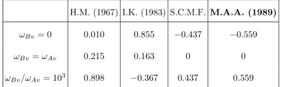
composition and the correlation factor for self-diffusion, f0. The corresponding expression of b coincides with equation (64) unless the constant (1 − ₁₁9) is replaced by the more general quantity (1 − f0). On the other hand a discussion given in (Nastar et al. 2000) predicts that equation (64) is quite satisfying as long as the exchange frequencies are not too different. Indeed the effective Hamiltonian is truncated after pair interactions and self-consistency is satisfied until two-point averages only. Time derivatives of N-point averages (N > 2) are proportional to (ωA− ωB). The larger the difference between effective frequencies the worse the self-consistency of kinetic equations. Indeed, it is observed that the difference between equations (63) and (64) increases with (ωA− ωB). In summary, we expect that a critical test of the present model will be the behaviour of b for high values of (ωBv − ωAv). For example, when ωBv (resp. ωAv) is taken to be zero, b(M.A.A.) is found to be equal to −0.559 (resp. 0.559) while the present b is equal to −0.437 (resp. 0.437).

[Insert table 1 about here]

However, table (I) shows that a relative error of around 20% on the value of b is not so critical compared to the errors made by the multi-frequency models which in some cases do not predict the right sign even. The enhancement factor should vanish when jump frequency of solute is equal to the solvent jump frequency which is verified by all the random alloy model and the present model but not by the five frequency models. It is even more surprising that an improved calculation (Ishioka and Koiwa 1984) which considers larger radius for the estimation of the partial correlation factors appears to be worse than the initial approximation of H. M. (1967). Note that the predictions of Lidiard 1 2 3 4 5 6 7 8 9 10 11 12 13 14 15 16 17 18 19 20 21 22 23 24 25 26 27 28 29 30 31 32 33 34 35 36 37 38 39 40 41 42 43 44 45 46 47 48 49 50 51

For Peer Review Only

(1960) are not given in table (I) since it would give 0 at any value of the jump rates. As a conclusion already noted down by Allnatt and Lidiard (1987) and recently confirmed by Monte Carlo simulations of Belova and Murch (2003), the multi-frequency models are inaccurate when they are used to predict the effect of solute on self-diffusion in a random alloy.

B. The fcc interacting alloy

In opposition to the last five-frequency models (Howard and Manning 1967, Ishioka and Koiwa 1984), the present model provides with an analytical expression of b (equations (56) and (57)). As shown by Howard and Manning (1967), the enhancement factor depends on three ratios, ω_Av3 /ω1_Av, ωBv/ω_Av1 and ω_Av4 /ω_Av0 . The two first ratios represent the relative probabilities of the possible jumps a vacancy can make when it is at a nn site of a solute atom. And the last ratio, ω4_Av/ω0_Av represents the relative probability of the jumps a vacancy can make when it is at a next nn site of a solute atom. The ratio ω4

Av/ω3Av which determines the probability of forming a pair Bv is not involved as long as sinks and sources of the system manage to maintain the vacancy concentration in the matrix at the corresponding value in pure A. We shall limit the discussion to the comparison between the present model and the previous five frequency models. No comparison is possible with other mean field approaches such as the Path Probability Method (Sato and Kikuchi 1983) and the Taylor series expansion of the time correlation functions (Qin et al. 1998) or more empirical techniques (Stolwijk 1981, Bakker 1979) since no one makes appear the five jump frequencies in the dilute limit.

Although, the Lidiard model (1960) is limited to the description of the effect of solute on the mean solvent jump frequency (bω), it is represented in the figures so that the correlation effect contribution, 1 2 3 4 5 6 7 8 9 10 11 12 13 14 15 16 17 18 19 20 21 22 23 24 25 26 27 28 29 30 31 32 33 34 35 36 37 38 39 40 41 42 43 44 45 46 47 48 49 50 51

For Peer Review Only

bf, can be directly measured by making the difference with the values of Lidiard. Note that the MC simulations and every theory agree on the estimation of bω, the discrepancies with the MC results are due to an approximate estimation of the correlation effects.

The jump frequency of solutes can have a significant effect on the self-diffusion by modifying its correlation factor. This effect is omitted by the first model of Lidiard (1960) which is limited to b = bω (equation (56)). The SCMF model predicts an increasing of b with ωBv/ωAv1 no matter the value of ω3_Av/ω1_Av and ω_Av4 /ω_Av0 . Indeed ∂b ∂(ωBv ω1 Av ) = 4(1 − 9 11)( ω_Av4 ω0 Av )(ω 3 Av ω1 Av ) (8ω 1 Av ω3 Av − 17)2 (9ωBv ω1 Av + 7ω3Av ω1 Av + 2)2 (65)

is always positive. This tendency already predicted by H.M. (Howard and Manning 1969) is in agree-ment with the Monte Carlo simulations (figures (1) and (2)). We choose to represent MC simulations of Belova and Murch (2003a) in figure (2) to explore a new set of jump frequencies but also to make sure that a positive variation of b with ωBv/ωAv1 is verified by different authors. The SCMF theory predicts a very small variation of b in agreement with the MC simulations while it underestimates the slowing down of self-diffusion due to correlation effects. Calculation of I.K. (Ishioka and Koiwa 1984) was proved to be not accurate in the random alloy limit. Figures (1) and (2) reveal that it is still not accurate when it is examined in the region where the various host atom jump frequencies are close to one another. Moreover, the prediction of a negative slope of b with respect to ωBv/ωAv1 extends beyond the set of frequencies represented in figures (1) and (2)) : at ω_Av4 /ω_Av0 = 0.1 and ω_Av3 /ω_Av1 > 0.1 ; and also at ω_Av4 /ω_Av0 = 1 and 0.25 < ω_Av3 /ω_Av1 < 5. For some values of the jump frequencies, the curves of I.K. and H.M. are above the curve associated to the Lidiard theory (1960) and predict then a speed up of the self-diffusion coefficient by the correlation effects, which is in contradiction with the MC 1 2 3 4 5 6 7 8 9 10 11 12 13 14 15 16 17 18 19 20 21 22 23 24 25 26 27 28 29 30 31 32 33 34 35 36 37 38 39 40 41 42 43 44 45 46 47 48 49 50 51

For Peer Review Only

simulations.

[Insert figure 1 and 2 about here]

The fall of b at low values of ω_Av3 /ω1_Av is a general feature occurring at any value of the other two ratios (figure (3) and Belova and Murch 2003a).

[Insert figure 3 about here]

A schematic representation given in figure (4) helps to understand the role of correlations in relation with the range of the effective interactions. It represents the possible jumps of a vacancy after a first jump with a tracer in a fcc lattice. Two initial jumps are represented, ω1 (case a)) and ω0 (case b)). In both cases, low values of ω_Av3 /ω_Av1 enhance the jump back of the vacancy in opposition to the escaping jumps which lead to a slowing down of the self-diffusion by the correlation effects. The role of the nn effective interactions appears clearly in equation (9). They require to determine what are the chemical species on the nn sites of the migrating atom (tracer). In figure (4), the solute atom of case a) is seen by the effective interactions since it is nn of the tracer but not the one of case b). We understand then that some of the correlation effects are missed by the SCMF when the effective hamiltonian is restricted to nn effective interactions. Ishioka and Koiwa (1984) which consider longer paths of the 1 2 3 4 5 6 7 8 9 10 11 12 13 14 15 16 17 18 19 20 21 22 23 24 25 26 27 28 29 30 31 32 33 34 35 36 37 38 39 40 41 42 43 44 45 46 47 48 49 50 51

For Peer Review Only

vacancy and more details of the local environment around the vacancy is more efficient to describe such a strong correlation effect.

[Insert figure 4 about here]

The MC simulations of figure (5) reveal a non-monotonous variation of bf with respect to ω4Av/ω0Av. Indeed at values of ω4_Av/ω_Av0 above 5, correlations effects enhance the self-diffusion. Note that this phenomenon was not observed by Belova and Murch (2003a) perhaps because self-diffusion was not studied for values of ω_Av4 /ω_Av0 beyond 5. H. M. and I. K. overestimate the slowing down due to correlation effects and do not predict the reverse trend at higher values of the ratio ω_Av4 /ω_Av0 , while the present theory predicts a bf equal to zero which appears to be a better approximation of bf. Although the present model moves away from the MC simulations at higher values of ω_Av4 /ω0_Av. An acceleration of self-diffusion by the correlation effects means that the solvent correlation factor is higher than f0 but still below 1.

[Insert figure 5 about here]

A schematic diagram drawn in figure (6) represents the possible paths of a vacancy after a ω3 or a ω0 jump type. Note that in the case of an alloy simulated by the third parameter set (defined in section 1 2 3 4 5 6 7 8 9 10 11 12 13 14 15 16 17 18 19 20 21 22 23 24 25 26 27 28 29 30 31 32 33 34 35 36 37 38 39 40 41 42 43 44 45 46 47 48 49 50 51

For Peer Review Only

IV), initial jumps of type ω1 and ω4 would show no preferential path of a vacancy. Figure (6) shows that in both cases a high value of ω4/ω0 enhances the escape frequency of a vacancy compared to a coming back. It is natural then to observe an acceleration of the self-diffusion by the correlation effects. Note that the nn effective interactions do not see the solute atom so that the vacancy follows a random path after the initial jump which explains that the SCMF curve meets the Lidiard curve in figure (5).

[Insert figure 6 about here]

The model has been successfully tested in the region of the random alloy (figures (1) and (2)). In an interacting alloy, the SCMF results are observed to be in reasonable agreement with the MC simulations and well reproduce the main tendencies : large slowing down of the self-diffusion due to correlations at low ratio ω3/ω1 and weak correlation effects in an alloy associated to the third parameter set (figure 5). Moreover, the limitations of the model are easily connected to the range of the effective interactions considered. A significant improvement of the model would be obtained if the effective Hamiltonian was extended to the next nearest neighbour effective interactions.

VI. CONCLUSION

SCMF kinetic equations based on an atomic model of atom-vacancy exchange frequencies are written in the general case of a multi-component alloy with any crystallographic structure. They lead to an 1 2 3 4 5 6 7 8 9 10 11 12 13 14 15 16 17 18 19 20 21 22 23 24 25 26 27 28 29 30 31 32 33 34 35 36 37 38 39 40 41 42 43 44 45 46 47 48 49 50 51

For Peer Review Only

expression of the phenomenological coefficients as a function of time dependent effective interactions which are solved using the the kinetic equations of the next moments of the distribution function under steady state conditions. An explicit calculation is carried out for the case of a fcc matrix of A atoms containing a small amount of B atoms and isotope atoms (A∗). The phenomenological coefficients, LAA, LAB and LBB, are equivalent to the first shell formulae of the five-frequency model (Howard and Lidiard 1963, 1964). A new analytical model for evaluating the effect of solute atoms on the self-diffusion coefficient is given. In the particular case of a random alloy, the present SCMF approximation is found to be equivalent to a previous formulation based on a lower statistical approximation but valid at any concentration of a multi-component alloy. In agreement with the Monte Carlo simulations the self-diffusion coefficient is increasing with the solute jump frequency in opposition to the previous five-frequency model (Ishioka and Koiwa 1984). Although a good quantitative agreement is obtained (within 20 %), the discrepancy is recognized to be due to the fact that pair effective interactions are considered only with a neglect of the triplet interactions. In an alloy with interactions, the SCMF prediction of the self-diffusion coefficient reproduces the main tendencies of the Monte Carlo simulations based on the same atomic model, with in general, a better agreement than the previous five-frequency models. When the quantitative agreement is not satisfying (for example at low ratio of ω3/ω1), it can be explained by the fact that nearest neighbour effective interactions are considered only which greatly reduces the level of description of the diffusion paths offered to a vacancy after a first exchange. As a consequence the main discrepancies can be easily corrected by an extension of the effective Hamiltonian to interactions with a larger range. This approach is promising since it reconciles a diffusion model devoted to concentrated alloys with a multi-frequency approach usually restricted 1 2 3 4 5 6 7 8 9 10 11 12 13 14 15 16 17 18 19 20 21 22 23 24 25 26 27 28 29 30 31 32 33 34 35 36 37 38 39 40 41 42 43 44 45 46 47 48 49 50 51

For Peer Review Only

to dilute alloys. The objective will be to give a multi-frequency formulation of the phenomenological coefficients of a concentrated alloy. It will allow to predict negative values of the non-diagonal transport coefficients which is not possible with the actual diffusion models of concentrated alloys.

APPENDIX A

Following equation (3), the distribution function is divided into two terms : dhnα_inβ_jnγ_k. . .i dt = X s6=i6=j6=... hnβ_jnγ_k. . . [nα_snv_iωb αv si − nαinvsωb αv is ]Pb₁(n, t)i(0)+ X s6=i6=j6=... hnα_inγ_k. . . [nβ_snv_jωb βv sj − n β jn v sωb βv js]Pb₁(n, t)i(0)+ . . . , (66)

where h. . .i(0) means averaging over the equilibrium distribution function Pb₀(n). Expansion of Pb₁(n)

to first order in bh(t) and δµ(t) gives :

dhnα in β jn γ k. . .i dt = X s6=i6=j6=... hnβ_jnγ_k. . . [nα_snv_iωb αv si − nαinvsωb αv is ](1 + β(δΩ(t) + X α,i δµα_i(t)nα_i −bh(t)))i(0)+ X s6=i6=j6=... hnα_inγ_k. . . [nβ_snv_jωb βv sj − n β jnvsωb βv js](1 + β(δΩ(t) + X α,i δµα_i(t)nα_i −bh(t)))i(0)+ . . . ,(67)

By construction of the exchange frequencies, detailed balance principle is satisfied at equilibrium :

b

P0(n)nαsnviωb

αv

si (n) =Pb₀(n0)n0α_in0v_sω_bαv_is (n0), (68)

where configurations n and n0 differ by an exchange of atom α on site i and a vacancy v on a neighbouring site s. Equation (68) summed over all the configurations leads to the equality :

hnα_snv_iωb αv si i(0) = hnαinvsωb αv is (n)i(0). (69) 1 2 3 4 5 6 7 8 9 10 11 12 13 14 15 16 17 18 19 20 21 22 23 24 25 26 27 28 29 30 31 32 33 34 35 36 37 38 39 40 41 42 43 44 45 46 47 48 49 50 51

For Peer Review Only

Therefore to first order in bh(t) and δµ(t), equation (67) simplifies to :

dhnα in β j . . .i dt = β X s6=i6=j6=... hnβ_j . . . [nα_snv_iωb αv si (δµαs − δµαi −bhα_s +bhα_i)i(0)+ β X s6=i6=j6=... hnα_i . . . nα_inβ_snv_jωb βv sj(δµβs − δµ β j −bhβ_s +bhβ_j)i(0)+ . . . . (70)

Note that δΩ(t) disappears in the difference.

APPENDIX B

The calculation consists in dividing the sums into blocks of equivalent four-point averages and by using the antisymmetry property of the effective interactions summing each block in terms of the positive first nearest neighbour effective interaction. The estimation of each sum is listed in table (II), each cell corresponding to a summation over p indices at fixed site s. To get the final result it suffices to sum the equivalent four-point averages over s. For example first term of the rhs of equation (25) results from the sum of the first three cells of the first column, each cell being weighted by the number of equivalent s sites : [(−4) ∗ 1 + (−2) ∗ 2 + (0) ∗ 4v_(ασ)1](v_(ασ)1/v_(ασ)1).

[Insert table 2 about here]

ACKNOWLEDGMENTS

The authors are grateful to V. Barbe, P. Bellon, J. L. Bocquet, E. Clouet, B. Legrand, G. Martin and F.Soisson, for their judicious comments and their assistance.

1 2 3 4 5 6 7 8 9 10 11 12 13 14 15 16 17 18 19 20 21 22 23 24 25 26 27 28 29 30 31 32 33 34 35 36 37 38 39 40 41 42 43 44 45 46 47 48 49 50 51