Dynamique d'aimantation dans les jonctions tunnels magnétiques à anisotropie perpendiculaire

HAL Id: tel-00967000

https://tel.archives-ouvertes.fr/tel-00967000

HAL is a multi-disciplinary open access archive for the deposit and dissemination of sci-entific research documents, whether they are pub-lished or not. The documents may come from

L’archive ouverte pluridisciplinaire HAL, est destinée au dépôt et à la diffusion de documents scientifiques de niveau recherche, publiés ou non, émanant des établissements d’enseignement et de

Thu Nhi Tran Thi

To cite this version:

Thu Nhi Tran Thi. Dynamique d’aimantation dans les jonctions tunnels magnétiques à anisotropie perpendiculaire. Materials Science [cond-mat.mtrl-sci]. Université Joseph-Fourier - Grenoble I, 2009. English. �tel-00967000�

T

HÈSE

presentée par

Thu-Nhi T

RAN

T

HI

En vue de l’obtention du grade de

D

OCTEUR DE L

’U

NIVERSITÉ

J

OSEPH

F

OURIER

(loi du 30 mars 1992)

Spécialité : Physique de la Matière Condensée et du Rayonnement

Dynamique d’aimantation dans les

jonctions tunnels magnétiques à

anisotropie perpendiculaire

Défendue publiquement le 16 juin 2009

Jury

Messieurs D.

R

Rapporteur

S.

M

Rapporteur

A.

S

Madame A.

M

Messieurs Y.

S

P.

W

Cette these a été effectuée au

T

ABLE OF CONTENTS

1

Fundamentals and concepts of Domain wall Propagation and

MTJ with epitaxial barrier... 13

1.1 Introduction on the study on magnetic domain wall ...14

1.2 Theory of magnetic domains and domain walls ...15

1.2.1 The basis of wall motion and Landau-Lifshitz theory...16

1.2.2 Gilbert Damping factor ...16

1.2.3 Domain wall dynamics in one dimension...17

1.2.3.1 Moving domain wall ...17

1.2.3.2 Walker breakdown ...18

1.2.3.3 Creep and flow regimes of domain wall motion with perpendicular anisotropy ...19

1.2.3.4 Wall velocity and stability in systems of reduced dimensions ...20

1.2.4 Review of the propagation process in the perpendicular anisotropy thin film ...21

1.3 MTJ with epitaxial barrier ...22

1.4 FePt alloy ...26

2

Experimental techniques and simulation used... 29

2.1 MBE system ...30

2.1.1 Description of MBE system ...30

2.1.2 Description of the used chamber...31

2.1.2.1 Description of the e-beam ...31

2.1.3 Thickness control...31

2.1.4 Sample cleaning...31

2.1.4.1 Ex-situ cleaning ...31

2.2 Principle of X-Ray Diffraction ... 32

2.3 The vibrating sample magnetometer VSM technique... 33

2.4 Magneto – optical effect ... 34

2.5 Kerr polar Microscopy MOKE... 36

2.5.1 Polar Kerr Microscopy Set-Up (in LPS) ... 36

2.5.2 Magnetic Field Pulse Generation... 37

2.5.3 Recording Magneto-optical Images... 39

2.5.4 Optical resolution and magneto-optical contrast... 40

2.5.5 Experimental method to study domain wall velocity... 40

2.6 Simulation method for domain wall motion with perpendicular magnetization... 41

3

Growth, structural and magnetic characterizations...43

3.1 Growth process... 44

3.1.1 Description of the growth of each layer ... 44

3.1.2 Growing conditions... 45

3.2 Structural characterizations ... 46

3.2.1 Anisotropy of FePt thin film ... 47

3.2.2 Magnetic characterizations ... 48

3.2.3 A few words on FePt/MgO/FePt tunnel junction transport properties ... 50

3.3 Conclusion... 51

4

Magnetization dynamic and Domain wall propagation in FePt

single layer...53

4.1 Study of propagation of magnetic domain walls in FePt single layer ... 54

4.1.1 At thickness from 2 to 5 nm... 54

4.1.1.1 Propagation depending on field ... 54

4.1.1.2 Time dependent propagation ... 58

4.1.1.3 Demagnetization state ... 61

4.1.1.4 Conclusion... 62

4.1.2 Domain decoration when increasing thickness ... 62

4.1.2.1 Observing the vestigial 360° winding wall ... 63

4.1.2.2 Propagation at low field ... 64

4.1.2.3 Propagation at high field ... 65

4.2 Study on domain wall velocity in FePt single sample ... 67

4.2.1 Introduction ... 67

4.2.2 Domain wall velocity in FePt single layer with different thickness ... 68

4.2.2.1 The quick view from experiment data... 69

4.2.3 Calculations from hypothesis of the regime where experiment data stay for single sample 70 4.2.3.1 The first hypothesis: we are in the regime with Walker breakdown. ... 70

4.2.3.2 The second hypothesis: we are in the precessional regime above the Walker breakdown ... 73

4.2.4 Simulation of domain wall motion with perpendicular magnetization ... 75

5

Magnetization dynamic and DW motion in FePt/MgO/FePt MTJ...81

5.1 Study on propagation of magnetic domain walls in MTJ sample...82

5.1.1 Applying field around the first reversal ...83

5.1.2 Applying field between reversal of the soft layer and of the hard layer ...85

5.1.3 Around the second reversal: 2.32 kOe...88

5.1.4 Demagnetization...89

5.1.5 Conclusion ...91

5.2 Study on domain wall velocity in MTJ sample...91

5.2.1 MOKE results for domain wall velocity in MTJ sample ...91

5.2.2 Comparison between MTJ sample and 5nm MTJ sample ...93

5.2.3 Analysis of the experimental results of DW propagation in MTJ ...94

5.2.4 Conclusion ...95

5.3 Demagnetizing the hard layer by cycling the soft layer ...96

5.3.1 Introduction...96

5.3.2 Kerr effect experiment for cycling measurements ...97

5.3.2.1 Kerr- effect measurement...97

5.3.2.2 Observation of the demagnetization of the structure by cycling the soft layer ...98

5.3.2.3 Behavior of amplitude and centre of the minor loop during cycling process...100

5.3.2.4 Demagnetizing procedure under different value of applied field for cycling Hcyc 102 5.3.3 MFM experiment...105

5.3.3.1 MFM experiment at various points of the cycling experiment ...105

5.3.3.2 MFM experiments to observe domains of both soft and hard layer at lower applied field Hcyc = 1.8 kOe ...107

5.3.4 Mathematical analysis of the behavior of the centre and remanent amplitude during cycling...111

5.3.4.1 Formula for centre of minor loop...111

5.3.4.2 Formula for remanent amplitude of minor loop ...116

T

ABLE OF FIGURES

Fig. 1.1: Structure of a Bloch wall in a uniaxial crystal. The magnetization vector remains always

normal to the x direction. [LEE80] ... 15

Fig. 1.2: Structure of a Néel wall in a uniaxial crystal. The magnetization vector remains always parallel to the xz plane. ...15

Fig. 1.3: The figure shows a section of a 180° Bloch wall containing a vertical Bloch line (BL) in the centre. The magnetization directions indicated are those of the centre of the wall. The Bloch line carries a Bloch point (BP)... 15

Fig. 1.4: in a moving domain wall the magnetization is rotated upwards by the torque of the demagnetization field. The peak velocity is reached at

φ

π

φ

π

Fig. 1.5: Wall velocity mormalized to the Walker velocity Vw = ∆K’/M as as a function of drive field H for three values of damping α [MAL79]. ...19

Fig. 1.6: theoretical variation of the velocity [MET07]:... 19

Fig. 1.7: Sketch of a 180° domain wall's velocity as a function of an external magnetic field H. This cartoon indicates the two linear regimes of velocity, below and far above the Walker breakdown. The dotted line in the transient non-linear regime is a guide for the eyes. ... 20

Fig. 1.8: The calculated transmission probabilities as a function of k|| in the Fe(100)/MgO(100)/Fe(100) system for 8 ML MgO for:...24

Fig. 1.9: Tunneling DOS for k|| = 0 for Fe(100)/8MgO/Fe(100). ... 25

Fig. 1.10: Conductance as a function of the number of MgO layers [BUT01]...26

Fig. 1.11: FePt alloy ordered in the L10 phase. ... 28

Fig. 2.1: Scheme of the MBE system. ... 30

Fig. 2.2: in-situ cleaning process by heating with 5A current is considered to 550°C. ... 32

Fig. 2.3: Crystalline structure of MgO substrate... 32

Fig. 2.4: X-Ray Diffraction principle. ...33

Fig. 2.5: MOKE set up... 34

Fig. 2.6: Kerr Polar Microscopy Set-Up. ...36

Fig. 2.7: schema of the experiment with the various electronic apparatus... 37

Fig. 2.9: Computation modeling with the width w and the thickness t. ...41

Fig. 3.1: MTJ structure on subtract MgO (001). ...44

Fig. 3.2: RHEED patterns of the different layers of this structure...45

Fig. 3.3: Structural characterizations of Perpendicular MTJ ...47

Fig. 3.4: Hysteresis loop out of plane, in planeand difference of the two curves for 4 nm (a) and 2nm (b) FePt thin film...48

Fig. 3.5: Hysteresis loops of FePt layers with different thickness, measured by Kerr Polar effect under the perpendicular applied field. ...49

Fig. 3.6: Hysteresis loop of perpendicular MTJ. ...50

Fig. 3.7: a)I(V) curve at 300 K for a FePt/MgO(2 nm)/FePt junction in parallel configuration b) Conductance derived from curve a)...51

Fig. 4.1: PMOKE images of field evolution of the magnetic domain structure for sample FePt 2nm, starting from negative magnetization saturation:...55

Fig. 4.3: PMOKE images of single sample FePt 5 nm ...57

Fig. 4.4: PMOKE images of single sample FePt 5 nm under the high field during a short time ...58

Fig. 4.5: PMOKE images of time evolution of magnetic domain structure of single FePt(4 nm) layer under the same field: 1913 Oe...60

Fig. 4.6: PMOKE images of time evolution of magnetic domain structure of single FePt4nm layer under the high field: 2527 Oe. ...61

Fig. 4.8: PMOKE to observe vestigial domains for a 6 nm thick FePt layer ...62

Fig. 4.9: PMOKE for sample FePt 6 nm at low field...64

Fig. 4.10: PMOKE of ring decoration and magnetized channels in side for sample FePt 6 nm ...65

Fig. 4.11: PMOKE of sample FePt 6nm under the field H = 1700 Oe...66

Fig. 4.12: PMOKE of sample FePt 6 nm under the field H = 1770 Oe...66

Fig. 4.13: Domain wall velocity as a function of applied field with different thickness of FePt. ...68

Fig. 4.14: Domain wall velocity v = mH for different thicknesses of FePt in the hypothesis of steady regime with m = ( /α)...71

Fig. 4.15: Domain wall velocity v = mH with different thickness of FePt in hypothesis of precessional regime with m = /(α+α-1)+v0. ...73

Fig. 4.16: Time evolution of domain wall position and velocity...75

Fig. 4.17: Simulation of domain wall velocity versus field at several value of damping vector α....76

Fig. 5.1: Room temperature polar Kerr hysteresis loop of the MTJ structure. Only the decreasing field part has been measured. The other part was obtained by symmetry. ...82

Fig. 5.2: PMOKE images obtained from magnetic configurations under low fields...83

Fig. 5.3: PMOKE images of magnetic configurations with positive saturation +4.2 kOe ...84

Fig. 5.4: PMOKE image of the magnetic configuration after a field pulse: H = 1.803 Oe during Δt = 2 s...85

Fig. 5.5: PMOKE images showing the propagation of the soft layer and nucleation of the hard layer after different field pulses. For all the images, the indicated fields were applied during Δt = (0.3 + 0.8 + 1.2) µs...85

Fig. 5.6: magnetic stray field created above the domain wall in the soft layer within the hard layer.86 Fig. 5.7: PMOKE image of magnetic configurations starting with positive magnetic saturation: ....87

Fig. 5.8: PMOKE for sample FePt starting with negative magnetic saturation. ...88

Fig. 5.9: PMOKE images for magnetic behaviors of the hard layer. ...89

Fig. 5.10: PMOKE images of ac-demagnetizing. ...90

Fig. 5.11: Domain wall velocity, v, versus applied magnetic field H for the MTJ sample (red points are experimental data – blue line is only a guide for the eyes)...92

Fig. 5.12: Fitting velocity with two diffent regimes...95 Fig. 5.13: The change in remanent magnetization of the reference layers with numbers of field

normalized by the remanent magnetization MR, set at 5000 Oe before cycling or rotating. [GID98]...97 Fig. 5.14: Demagnetization of the MTJ by the cycling the soft layer between the field -Hcyc =

-1.83 kOe and Hcyc = 1.83 kOe. The angle of the Kerr signal is measured in µV... 98 Fig. 5.15: the evolution of remanent signal (amplitude of the loop on the zero field axis) and

centre of minor loop after 200 cycles with the applied field Hcyc = 1.9 kOe. The ellipticity of the Kerr signal is measured in µV ...100 Fig. 5.16: Demagnetization of hard layer by cycling the soft layer at different field and the evolution of centre and remanent amplitude of minor loop during cycling procedure ...103 Fig. 5.17: Centre of minor loop after normalization. ...104 Fig. 5.18: AFM image for the area where is taken MFM images. All the MFM images report after

were taken carefully at almost the same area of the same sample. ...104 Fig. 5.19: MFM images of magnetic configuration during cycling procedure with applied field

Hdeg = 2.0 kOe. ...105 Fig. 5.20: Cycling the soft layer at 1.8 kOe during 300 cycles. ...108 Fig. 5.21: Cycling the soft layer at 1.8 kOe during 30 cycles with some different value of Hend....108 Fig. 5.22: variations of the position of the centre in Kerr measurements during cycling. The fitting

curve is an exponential decay...111 Fig. 5.23: variations of the position of the centre in Kerr measurements during cycling. The two

fitting curves are exponential decays, one with a demagnetization parameter of 82 mV and the other one with a constrained value of 127 mV. ...112 Fig. 5.24: characteristic number of cycles during a demagnetization process versus the applied

field. The data shows an exponential behavior with a characteristic applied field H_0 = 0.12 kOe...114 Fig. 5.25: variations of the remanent amplitude of the cycle in Kerr measurements during cycling.

G

ENERAL INTRODUCTION

It has been just a year since spintronic was recognized as a major scientific achievement by the Nobel committee from the Swedish academy of science: in 2008, the committee awarded the Nobel Prize to Albert Fert and Peter Grünberg for their discovery of the giant magnetoresistance. Performed 20 years ago, this discovery opened the path to a tremendous increase in the bit density of hard drive disk that shifted from 20% per year to 60 % per year after the introduction of the spin valves in recording heads. It also led to the development of a new generation of memory device: the MRAM (for Magnetic Random Access Memory).

Such progresses and perspectives fueled and have been fueled by a huge interest and effort in research laboratories in the field of magneto-electronic. In the same period, some old subjects have been unearthed, and new discoveries made. Still now, magnetoelectronics is more than ever buzzing (to use a trendy world) and bursting with life, mostly because of a strong interplay between fundamental physics and applications. Certainly, the secret desire to uncover and to apply new concepts drives many researchers across the world.

We can trace the birth of spintronic to two main ideas. One is that in a naive picture the spin polarized current in a ferromagnet is carried by two currents - up and down spin carriers - flowing independently from each other. This is the “two currents” model from Mott. It is well known that the underlying hypothesis might not always be verified, but the Mott model allowed researchers to explain the resistivity curves of ferromagnets as the function of temperature. Other key aspects, often forgotten, are the major progresses made in the 70’s and the beginning of the 80’s for the growth of ultra thin films and multilayers. People around the world became able to grow stacks of materials with a better control of the interfaces, and with a higher intrinsic quality of each layers… One important discovery then made possible was the antiferromagnetic coupling between ferromagnetic layers in ferro-normal metal multilayers [GRU86]. This latter discovery was one of the key ingredients of the discovery of GMR [BAI88].

In 1995 Moodera and coworkers [MOO95] observed tunnel magnetoresistance at room temperature in alumina based magnetic tunnel junction (MTJ). This observation paved the way for another step in the information storage technology. It also led to the concept of MRAM

alumina based MTJ for the MRAM application. High voltage throughput, homogeneities on the scale of the silicon wafer, high TMR ratio were some of the issues tackled at that time.

I tried to show, with a few examples, that spintronic has been a very active field in the last 20 years. It has also revived the interest for magnetism in metal from slumber. Basic studies and technical progresses have both been helped by the invention of STM and of some linked techniques like Atomic Force Microscopy (AFM) and Magnetic Force Microscopy (MFM). Near field observation techniques and progress in patterning techniques enabled researchers to design and observe smaller and smaller structures down to the nanoscale. Theories have been tested, refined or rejected. One should never forget the importance of the technical progress in the advancement of science.

Most importantly regarding this thesis work, spintronics does not require the sole understanding of electronic transport, but also the fine mastering of magnetization phenomena in thin magnetic films, and in magnetic multilayers. Controlling magnetization reversal at an always reduced scale is indeed required to store and read information in all kind of magnetic devices.

For decades, the desire to anticipate the need of the storage industry for higher data densities pushed scientists to investigate more closely materials with strong perpendicular anisotropy. Such materials were used as model materials because they could be viewed as one-dimensional, at least with respect to some of their properties. They had hours of glory in the 70’s with the “bubble memory”. Many important theories were first introduced at that time. However, as the interest for bubble memory faded away, high perpendicular anisotropy materials were put back on the shelves of the laboratory. They were still used as model materials, but their use in magnetic media was regularly postponed by the progresses of longitudinal media. Finally, thin layers with perpendicular anisotropies are used in the magnetic hard disk since 2005.

Such thin films with perpendicular magnetic anisotropy offer a fascinating playground to the physicist:

- truly uniaxial perpendicular anisotropy can be readily obtained, either by building stackings with suitable interface anisotropy (such as Pt/Co/Pt trilayers), either by establishing uniaxial chemical ordering in chemically ordered alloys such as FePt. - there is a competition between the perpendicular magnetic anisotropy and the

magnetostatic field. This latter parameter favors in plane magnetization in thin films, but, when the perpendicular anisotropy is dominant, is at the origin of the formation of magnetic domains (and hence magnetic domain walls).

As a result, conversely to what is observed in systems with in plane magnetization, domain walls are not linked to a specific magnetic history and / or to sample defects, but are intrinsically part of the equilibrium magnetic state of the material. Indeed, the energy cost (anisotropy, exchange) related to the formation of the magnetic domain walls is compensated by a gain in the magnetostatic energy of the system when dividing the perpendicularly magnetized thin films in up and down domains [GEH97A, GEH97B, GEH99].

Let us now shift our discussion from thin layers to magnetic multilayers. Magnetic tunnel junctions are not focusing interest only because of the applied perspectives derived from their specific transport properties, or even because of the rich physics associated with spin filtering and induced by the epitaxial nature of the stacking. Indeed, in addition to electronic transport physics, Magnetic Tunnel Junctions also exhibit highly interesting magnetic properties, as being made of two ferromagnetic electrodes very close to each other. Average distance between the two ferromagnetic layers (thickness of the electrically insulating layer) is between 1 and a few nm. Practically, the question of a magnetic coupling between the two layers is of the utmost importance. Indeed, both spin valves based recording heads and MTJ based MRAM cells rely

on the magnetic stability of one of the two ferromagnetic electrodes, the so-called reference layer. Let us remind that this stability is ensured by exchange coupling of one of the magnetic layer (the reference layer) with an antiferromagnet in most devices.

In the case of MTJ with in plane magnetization, it has been shown that the hard layer can be demagnetized by cycling the soft layer – even when the cycling field is lower than the coercive field of the hard layer - at least in the absence of pinning by an antiferromagnet [GID98]. This has been explained by the action of the stray field created in the hard layer in the vicinity of the domain walls propagating in the soft layer during its magnetization reversal. Obviously, one could ask what will happen in MTJ with perpendicular magnetic layers, when stray field would be involved in both the interactions between magnetic layers and in defining the equilibrium size of the magnetic domains. Till now, similar studies are not numerous and the very few existing ones have been reported on spin valves - like magnetic systems [WIE06]. Nevertheless, these latter studies, often relying on MFM and Kerr observations, have shown that coupling between the two ferromagnetic electrodes gives rise to interesting magnetic patterns like decoration domains, domains mirroring… It is then tempting to investigate further this area. However almost nothing has been published on the dynamical properties of such systems, and this can be easily understood.

Indeed, until recently, the physics of domain wall propagation was of reduced interest for most of spintronics devices. MRAM cells or magnetic recording heads tended to rely on elements with a single domain configuration. This changed recently as new concepts of spintronics devices based on magnetic domain walls (DWs) have been proposed [ALL05], with the concept of racetrack memory emerging from the group of S. Parkin [PAR08]. In the most advanced designs, such memories would rely on the direct manipulation of magnetic walls using spin polarized electrical current (so-called Spin Transfer mechanism (ST)). This emerging field promises very low power consumption, simple architectures, ultra-fast operations, 3D stacking and thus has the potential to become a key technology for non-volatile memories and logic circuits. Here, materials with perpendicular magnetic anisotropy offer specific advantages as the large achievable anisotropy ends up with thin magnetic domain walls (a few nm in FePt thin films). So, thin domain walls are obviously desirable when targeting high data densities. They are also probably advantageous as the efficiency of current driven DW motion is probably strongly enhanced at such reduced domain wall widths.

These ideas currently fuel a strong interest in the physics of domain wall propagation in thin films with perpendicular anisotropy. Together with multilayers such as the widely studied Pt/Co/Pt, FePt is one of the preferred materials for such studies. Indeed, such alloys (FePt, FePd…) exhibit large optical effects, making these well-suited to use polar magneto-optical Kerr effect (MOKE) to study their magnetic properties in the static and dynamic cases. In addition, the large magnetization also facilitates local and high resolution observations by Magnetic Force Microscopy. Coupling both techniques then offer insight in the system properties combining time and spatial resolutions

This Phd work has then been focused on some emerging questions in these promising areas: - What can be said of the domain wall dynamics in thin films with perpendicular

anisotropy (FePt), going beyond the limit of the ultra-low thicknesses associated with the Pt/Co/Pt system?

- What are the phenomena occurring upon magnetization reversal in MTJ-like systems with perpendicular magnetization (FePt/MgO/FePt)?

We then focused our work on a thorough study concerning magnetic coupling between the hard and the soft layer of a fully-epitaxial Magnetic Tunnel Junction with perpendicular magnetization (FePt/MgO/FePt). In the first part of this manuscript, we start describing the fundamental concepts of magnetic domain walls in thin films with perpendicular magnetization as well as some theoretical elements on Magnetic Tunnel Junctions.

In the second part, we describe the main experimental techniques we used and some results common to both out-of-plane FePt single layers and FePt/MgO/FePt Magnetic Tunnel Junction. The third part reports on the growth and the basic characterization of the FePt thin layers and FePt/MgO/FePt MTJ.

The fourth part deals with FePt single layers with high perpendicular anisotropy. These studies are on two directions. First, the polar magneto-optic Kerr effect is used to observe the domain wall propagation on FePt single layer. Taking advantage of the bulk origin the magneto-crystalline anisotropy, the thickness of FePt was varied from 2 nm to 6 nm while preserving a large perpendicular anisotropy. Here, the behaviors of the domain wall are investigated in details. Second, the domain wall speed was measured as a function of the value of an applied perpendicular magnetic field. Then, the nature of the propagation regime was analyzed according to different hypothesis. Domain wall motion simulations are included confirming the analysis of the experimental data.

The fifth part deals first with similar studies on perpendicular magnetization FePt/MgO/FePt MTJ. We now focus on the additional complexity introduced by the coupling between the soft and the hard layer. Then, to answer the question about the interdependency between the two electrodes, Kerr – effect experiments were done to follow the magnetization of both magnetic layers when cycling the soft layer. Additional insight into the involved processes was provided by Magnetic Force Microscopy images. These images uncovered unique and unexpected magnetic patterns in the hard layer at intermediate stage of the demagnetization process.

1 Fundamentals and concepts of Domain wall

Propagation and MTJ with epitaxial barrier

1.1 Introduction on the study on magnetic domain wall

Magnetic domain walls (DWs) are one of the focus points for research in spintronic. The discovery that one could push DW [GRO02] with a current has renewed an already considerable interest in such objects. Because magnetic thin films and nanostructures needing no power to maintain magnetic states, it has been tried to use this ability either in reprogrammable logic [ALL05] or in memory devices like the MRAM or the racetrack memory [PAR08].

Static properties of magnetic domain walls have been investigated thoroughly. With the advance of microscopical techniques like Lorentz microscopy, magnetic force microscopy and kerr microscopy, a deep understanding has been achieved. The reader can refer to the book of Hubert and Schäffer [HUB98] to gain more insights into their properties. Our work has focused on the dynamic properties of high perpendicular anisotropy thin films. Therefore, I will only review the basic properties of out-of-plane domain wall (Bloch wall) in the first part of this chapter. In high perpendicular anisotropy thin films, domains take the form of bubble. In the 70’s, such a kind of domain was foreseen as the core of new memory devices. In spite of a strong effort from the community of magnetism, magnetic bubbles were abandoned. However this effort was transmitted to the future generation in one work that is the legacy of that era. The book of Malozemoff and Slonczewski [MAL79] is a “must read” to anyone interested in the dynamic properties of DW in high perpendicular anisotropy thin films. I will review the relevant ideas for our study in the second part of this chapter. I will introduce the different regimes of propagation that may be observed in our systems. A brief review of published experiments relevant to our work will also be presented.

In the racetrack device one way to measure the position of a moving DW is through its interaction with a sensing layer positioned above the DW. However the dynamic of coupled systems has not been studied in details. I will also review the published work on that topic. Finally, I will briefly introduce MTJ and why epitaxial MTJ have been such a revolution in the last 10 years.

1.2 Theory of magnetic domains and domain walls

Magnetic domains are formed into ferromagnetic materials to minimize the energy of the magnetic configuration. Several energy terms are to be taken into account to understand: crucial parameters for determining the size of the domains and the type of the boundaries between them are the shape of the sample, the saturation magnetization, the magnetic anisotropies… [LEE80]. Domain wall is the name by which we call the area of the sample that separate two adjacent domains with different magnetization orientations. We will restrict ourselves to the two basic types of domain walls: Bloch walls (Fig. 1.1) and Néel walls (Fig. 1.2).

Fig. 1.1: Structure of a Bloch wall in a

uniaxial crystal. The magnetization vector remains always normal to the x direction. [LEE80]

Fig. 1.2: Structure of a Néel wall in a uniaxial

crystal. The magnetization vector remains always parallel to the xz plane.

[LEE80]

In a 180° Bloch wall the magnetization vector rotates such that it always remains parallel to the plane of the wall. In a Néel wall the magnetization vector, while rotating, remains parallel to a plane normal to the wall. Néel wall may have a higher specific energy than the Bloch wall, due to the additional energy of the demagnetization field introduced by the free poles on the surface of the wall. In some cases, when the dimensions of the sample become comparable to the wall width, such as in thin permalloy films, the situation may reverse. Bloch and Néel walls have an additional degree of freedom: the sense of rotation may be clockwise or counter-clockwise. If in a Bloch wall both senses of rotation occur, the two wall type regions are separated by a Bloch

line (Fig. 1.3). A Bloch line is a string-like discontinuity. It may contain Bloch points which are

also shown in Fig. 1.3.

Fig. 1.3: The figure shows a section of a 180° Bloch wall containing a vertical Bloch line (BL)

in the centre. The magnetization directions indicated are those of the centre of the wall. The Bloch line carries a Bloch point (BP).

the total surface of the wall multiplied by the specific wall energy per unit area. For most static problems, the specific wall energy is considered to have a constant value unaffected by stray fields. The non-zero width of the walls is usually disregarded. The second part consists of the total magnetization energy due to the external magnetic field. The third contribution is the magnetization energy due to the stray field of the domains. In general, the latter contribution is the most complex to evaluate. It has only been calculated for a limited number of simple domain structures. One of the domain structures which has been studied in detail is the domain structure in thin platelets of a uniaxial crystal with a preferential direction normal to the platelet. It is this basic geometry which has been used for most of the experiments described in the present review.

1.2.1 The basis of wall motion and Landau-Lifshitz theory

The physical basis of the dynamic process of wall motion is the gyroscopic precession of the electronic spin. This property of the electron determines directly the macroscopic properties: the magnetization vector responds orthogonally to the torque acting on it. The rate of change of the direction of the magnetization M is described by the equation proposed by Landau and Lifshitz [MAL79]:

M

M

M

M

w

M

M

&

=

×

+

α

&

×

δ

δ

γ

This equation is the starting point for all discussions of bubble dynamics where = ge/2mc (> 0) is the gyromagnetic ratio and α is the dimensionless Gilbert damping factor.

The term

M&

M

M

M

&

×

α

“dynamic” terms because they contain a time derivative of M. By contrast the term

M

w

M

δ

δ

γ

×

essentially a static term. If this term is zero, then equation (1.1) can be satisfied with .

M

The effective field can be conveniently expressed as the sum of two terms thusly:

' M M M w H_e

γ

δ

δ

δ

In the general case with He not constant, the total energy represented by the volume integral of Ω is conserved when α = 0.

1.2.2 Gilbert Damping factor

Gilbert damping factor has been defined as the phenomenological coefficient of the non-conservative term of eq. (1.1).

For low damping, a « 1, equation (1.1) describes a precession of the magnetization around the magnetic field having angular frequency ω = / M. The damping term causes the precession angle to decrease.

For values of α » 1 both terms are equivalent. The damping terms introduced here are empirical in nature but have proven useful for the description of various phenomena, such as ferromagnetic resonance and domain wall dynamics [WAL56].

1.2.3 Domain wall dynamics in one dimension

1.2.3.1 Moving domain wall

An external magnetic field along the z axis favors the orientation of the magnetization in one of the domains. Accordingly this domain will tend to grow and thereby displace the domain wall. Determining the equation of motion of a domain wall starts by studying the equation of motion for the magnetization M(r, t):

)

,

(

)

,

(

t

r

T

t

t

r

M

γ

δ

δ

₌

₋

where γ is the gyromagnetic ratio and T(v,t) is the total torque density. It contains contributions from exchange, anisotropy, magnetic fields and damping.

The equations of motion can then be integrated for a uniformly moving wall (Walker 1956 and Schlomann 1972) and give:

2 / 1 2 1

)

cos

1

(

2

sin

2

Δ

+

=

γ

M

φ

Q

φ

v

Where the quality factor Q is defined by:

M H

M K

Q = _u /2

π

π

Where Ku is the uniaxial anisotropy constant.

Fig. 1.4: in a moving domain wall the magnetization is rotated upwards by the torque of the

demagnetization field. The peak velocity is reached at

φ

π

φ

π

The applied field does not exert a torque moving the magnetization upward. This role is fulfilled by the demagnetization field. The torque acting on the magnetization is then:

φ

φ

π

sin

cos

4

M

−

φ

φ

π

sin

cos

4

M

v

=

−

Δ

From this expression of the velocity of the wall, it will be clear that there is an upper limit to the wall velocity due to the finite value of the demagnetizing field. In materials with Q » 1 the wall has a peak velocity:

M

v

=

2

πγ

Δ

that is reached when

4

/

π

φ

=

φ

=

3

π

/

4

This peak velocity is usually referred to as the Walker limit.

Equating these results we find a linear relationship between the velocity and the drive field:

H

v

=

μ

with the mobility µ given by:

α

γ

μ

=

Δ

/

Or:

v

=

γ

Δ

H

/

α

The velocity is in this case inversely proportional to α. 1.2.3.2 Walker breakdown

The domain-wall velocity is sustained by a torque on the in-plane magnetization. And according to the two static types of Bloch wall [LEE80], they have:

M v q_{max W 0} . 2 Δ = ≡

πγ

with q is the wall displacement along the x axis and M is the saturation magnetization. The velocity occurs at a net drive field H[= Ha – (kq/2M-Hc)] of:

Hw = 2παM (1.10)

These are the important formulae for the “Walker breakdown velocity” vw and the “Walker critical field” Hw.

The critical velocity _max .

q in each of above cases corresponds to a critical drive field: 0 max . max . max =q /

μ

α

γ

Fig. 1.5 shows a plot of an analytic expression for the complete field dependence of the velocity average over a precessional cycle, for the case of demagnetizing an in – plane anisotropy torques. If the damping is small, the average velocity drops above the breakdown velocity and then increases again as the damping torque takes over. In the region of decreasing velocity or negative mobility, the domain wall is expected to be unstable, for if one area of the wall begins to lag, it experiences an increasing drive that, in this negative mobility region, will cause it to lag even further. Clearly the one dimensional model is inadequate to describe such behavior. If the damping is large (α » 1), the nonlinearity in V versus H is suppressed altogether (see in Fig.

Fig. 1.5: Wall velocity normalized to the Walker velocity Vw = γ∆K’/M as as a function of drive

field H for three values of damping α [MAL79].

1.2.3.3 Creep and flow regimes of domain wall motion with perpendicular anisotropy

Two theoretical variations of the velocity [MET07] are shown in Fig. 1.6. The dynamics of an elastic interface driven trough a weakly disordered medium by an applied force is a challenging problem relevant to many physical systems such as domain walls in ferromagnetic and ferroelectric materials. While theory predicts three main regimes of motion only the low force regime of creep has been experimentally studied through direct observation of the interface, regimes beyond that of creep, namely depinning and flow, have however been evidenced indirectly via ac susceptibility measurements ([CHE02] and [KLE07]).

Fig. 1.6: theoretical variation of the velocity [MET07]:

a) Theoretical variation of the velocity, v, of a 1D interface (domain wall) in a 2D weakly disordered medium submitted to a driving force, f (magnetic field, H), at zero and finite temperature, T. The creep, depinning and flow regimes are labeled.

b) Regimes of domain wall flow motion in an ideal ferromagnetic film without pinning. The steady and precessional linear flow regimes are separated by an intermediate

regime which begins at the Walker field, HW.

transition occurs (Fig. 1.6a) At finite temperature the depinning transition becomes smeared due to thermal activation and a finite velocity is then expected for all non-zero forces. This is true even for f << fdep where the thermally activated interface motion is known as creep. At the other extreme, once f is sufficiently beyond fdep, disorder becomes irrelevant resulting in a dissipative viscous flow motion with v ≈ f. Finally, between the creep and flow regimes, a transitory depinning region is expected. In magnetic domain wall motion experiments, the applied magnetic field, H, plays the role of a force, f. The film’s nanoscale inhomogeneties create the disorder which pins the wall and the domain wall energy provides the elasticity.

1.2.3.4 Wall velocity and stability in systems of reduced dimensions

According to [MOU07], the average velocity far above the Walker breakdown is simply given by: H

v

α

α

γ

is the gyromagnetic ratio

∆ is characteristic domain wall width. It is a normalized value taken into account of a thin film with a small given value of thickness of the thin film.

u has the dimension of a velocity and scales as the electrical current density.

• This regime is similar to the usual high field one described for a 180° Bloch wall. The average velocity is linear with the field, following an initial drop in the mobility at the breakdown.

Fig. 1.7: Sketch of a 180° domain wall's velocity as a function of an external magnetic field H.

This cartoon indicates the two linear regimes of velocity, below and far above the Walker breakdown. The dotted line in the transient non-linear regime is a guide for the eyes.

In a one-dimensional statement of wall motion, without current, a qualitative understanding of the damping/demagnetizing interrelation is easy to provide. When a drive field is applied along the anisotropy direction, M starts a φ precession movement, and tilts away with respect to its equilibrium orientation at rest, The component of the magnetization outside of the xz wall plane creates magnetic charges. The θ component of the torque resulting from the induced magnetostatic field describes the resulting additional precession of the spin around Hd.

anymore. Then, above the Walker field, the motion is characterized by an oscillation around an equilibrium position. In the presence of damping, the forward movement is favored and thus the equilibrium position moves on.

1.2.4 Review of the propagation process in the perpendicular

anisotropy thin film

Up to now, many studies on the propagation process in the perpendicular anisotropy thin film have been performed. The knowledge of dynamic behavior then developed strongly over the last decades. Lately this knowledge has also been used to study possible coupling between magnetic layers separated by a spacer layer. Recently, the group of Jacques Ferré from the Laboratoire de Physique des Solides at Orsay University obtained significant breakthroughs over the previous knowledge by imaging domain wall propagation with their MOKE experimental system. We report below some of the studies they have performed to provide to the reader a full picture of the recent studies of the propagation process in perpendicular anisotropy thin film study.

1. Their first report on the MOKE experiment study of high field DW dynamic is in Au/Co/Au films with perpendicular anisotropy [KIR93]. The Gilbert damping factors are derived from the study of DW velocity. The variation of DW velocity vs. the applied magnetic field can be distinguished by three regimes. They estimated approximate value of Gilbert damping from the viscous DW motion regime. The DW velocity in their case revealed the same qualitative behavior as in thicker bubble film or in bulk materials: at low field thermally activated jumplike motion, viscous motion at higher field (even if the relationship between the velocity and the field was not linear). Continuing with the same system, in [FER97] they reported on the magnetization reversal process, starting from an initial demagnetized state. The dynamic of the magnetization reversal is much faster for the indirect process since it is initiated from quasi-homogeneous “Swiss cheese” domain state with small non reversed region which act as nucleation centers when the magnetic field is subsequently reversed. The distribution function of local coercivities can then be determined from the experimental field dependence of the domain wall velocity. As in thicker film, a direct consequence of a nanoscale distribution of the coercivity is domain – boundary jaggedness.

2. Dynamic studies of two ferromagnetic layers separated by a non magnetic one, like spin-valve or MTJ have not attracted much attention. One must say that any coupling between the two layers complicate significantly the interpretation of the experiment. It is then desirable to be able to study each layer individually. Bonfin and coworkers [BON01] used X-ray magnetic circular dichroism (XMCD) at different element edges to observe independently the reversal of the two layers in a Co/Al2O3/Ni80Fe20 MTJ in the nanoscale range. They showed that the coupling between the two layers may differ between the static regime and the dynamic regime they could observe.

Fukumoto and coworkers [FUK06] used XMCD and X-ray photoemission electron microscopy on the same system to demonstrate the role of domain wall energy on the magnetization reversal of the soft layer in these MTJs. They observed that when the domains are small (perimeter below 2 µm) there is a delay in the domain expansion.

[WIE06]. They clearly showed the influence of dipolar coupling into the domain left in the remanent state, observing how domain decoration expands over time, even in the absence of any applied field. Moreover, at high field, the suppression of 360° domain walls in perpendicular system was reported.

4. In 2007, P. Metaxas et al [MET07] studied the domain wall velocity in ultrathin Pt/Co/Pt films with perpendicular anisotropy. For the first time, the complete velocity-field characteristics of a 1D interface in a 2D weakly disordered medium was reported, and obtained through direct measurements of domain wall motion in ultrathin Pt/Co/Pt films. The transition between thermally activated creep and viscous flow motion regimes - as predicted from general theories for drive elastic interfaces in weakly disordered media - are experimentally observed in this study. The authors also determined the value for the magnetic damping parameter based on the hypothesis of DW velocity staying in the precessional regime, which describes the dissipation occurring during flow motion.

Worth noting, almost nothing has been published on coupled systems, such as Magnetic Tunnel Junctions or Spin Valves systems. In such cases, two magnetic layers are separated by a thin insulating or metallic layers, whose thickness is in the nm range. Such a configuration results in unique behaviors as the two magnetic layers may strongly interact through the stray field creating by one of these on the other. If other interactions, such as RKKY coupling, may be significant in some specific cases, these are not to be considered in our systems. Finally, we emphasize that published studies (such as the one cited above) were performed in spin-valve like magnetic systems, while we are not aware of any detailed studies of the dynamics of coupled magnetic layers in magnetic tunnel junctions.

Metaxas et al [MET08] have conducted domain wall velocity measurement in coupled spin valve made of two ultrathin Co films separated by a 4 nm thick Pt spacer. The coupling manifests itself in the asymmetry between positive and negative driving field in the velocity measurement.

1.3 MTJ with epitaxial barrier

The magnetoresistance of magnetic tunnel junctions (MTJ) is of uncontested interest for key applications with, in particular, promising perspectives for the fabrication of nonvolatile memories: Magnetic Random Access Memories (MRAM). Till 1995 most studies have been performed on MTJs with a layer of amorphous alumina as insulating barrier between the ferromagnetic electrodes. Building upon continuous progresses, these studies produced systems with large and reproducible tunneling magnetoresistance (TMR), typically 50% at room temperature [TSY03].

The theoretical picture is far more complex in systems with an epitaxial barrier. Indeed, a correct depiction of the spin-dependent tunneling properties of epitaxial MTJs must transcend the simple potential barrier image and take into account the interplay of electronic structure between metal and insulator. A test of these models can be performed on single-crystal epitaxial grown structures. Towards this end, much work has been dedicated to characterize the growth and electrical behavior of ultra thin MgO layers. The interest for MgO based MTJ comes from the seminal work of Butler and collaborators. It is this work that has initiated the vast interest in MgO based MTJ.

One of the simplest theoretical model systems is an epitaxial Fe(100)/MgO(100)/Fe(100) sandwich which is formed of two infinite stacks of Fe layers corresponding to the leads on either side of the barrier. Moreover, the Fe-MgO system provides a good template for experimental work because the Fe-MgO interface is such that Fe or MgO thicknesses can be reduced to a few atomic layers while preserving a good epitaxy.

The following theoretical description of the tunneling process in Fe/MgO/Fe sandwiches is taken from a recent publication of MacLaren et al., which provides a reasonable theoretical approach for tunneling in layered epitaxial systems [BUT01]. The basic messages are:

• The tunneling conductance depends strongly on the symmetry of the Bloch states in the electrodes and of evanescent states in the barrier.

• Bloch states of different symmetry decay at different rates within the barrier. • There may be quantum interference of the decaying states in the barrier.

• Interfacial resonance states can allow particular Bloch states to tunnel efficiently through the barrier.

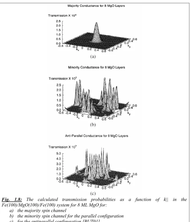
In Fe(100)/MgO(100)/Fe(100) quite different tunneling mechanisms may dominate the conductance in the two spin channels. In Fig. 1.8 the calculated transmission probabilities are shown as a function of k|| for (a) the majority spin channel and (b) the minority spin channel for the parallel as well as (c) for the antiparallel configuration of 8 layers of MgO. For the majority channel in Fig. 1.8a the conductance has a rather broad peak at k|| = 0. A somewhat similar peak is predicted for the tunneling of free electrons through a simple square barrier. The conductance has also an increasing amplitude of transmission near k|| = 0 as the insulating barrier layer is made thicker.

Fig. 1.8: The calculated transmission probabilities as a function of k|| in the

Fe(100)/MgO(100)/Fe(100) system for 8 ML MgO for: a) the majority spin channel

b) the minority spin channel for the parallel configuration c) for the antiparallel configuration [BUT01]

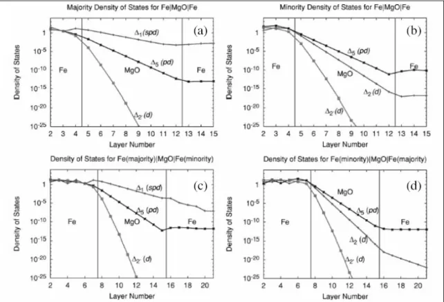
For a further clarification of the conductance process, the tunneling density of states (TDOS) has been examined, defined as the density of electron states subjected to the following boundary conditions. On the left-hand side of the interface there is an incoming Bloch state with unit flux and a reflected state. On the right-hand side are the corresponding Bloch states.

Fig. 1.9 [ZHA04] shows the TDOS associated with each of the Fe(100) Bloch states having

k|| = 0. Both the majority (Fig. 1.9a) and the minority (Fig. 1.9b) channels have four Fe(100)

Bloch states for k|| = 0. In the majority channel there is a Δ₁ state, a double degenerated Δ₅ state, and a Δ state. The minority channel has four states with the same symmetries as the states of

the majority channel with the exception that the majority Δ₁ state is replaced by the Δ₂ minority state. Only the majority channel has a slowly decaying Δ₁ state, therefore, its conductance is much higher than the one of the minority channel. The next slowest decay is that of the Δ₅ states which are present in both channels. Both Fe channels have a Δ2 state that couples to a Δ2 state in the MgO barrier where it rapidly decreases because there are no real Δ2 bands near the Fermi energy.

Fig. 1.9: Tunneling DOS for k|| = 0 for Fe(100)/8MgO/Fe(100).

The four panels show the tunneling DOS for majority (a), minority (b), and ant parallel alignment of the moments in the two electrodes (c) and (d). Additional Fe layers are included (c) and (d) to shown the TDOS variation in the Fe. Each TDOS curve is labeled by the symmetry of the incident Bloch state in the left Fe electrode [ZHA04].

Fig. 1.10 demonstrates that for all thicknesses the majority conductance overwhelms the minority and the antiparallel conductance because of the slow decay of the Δ1 states in MgO, leading also to an increasing TMR as the barrier thickness increases. Nevertheless, for thinner barriers the minority and antiparallel conductance are much closer to the majority conductance than for thicker barriers emphasizing the importance of the interfacial resonance states for very thin barriers.

Fig. 1.10: Conductance as a function of the number of MgO layers [BUT01]

1.4 FePt alloy

Strong uniaxial anisotropy is important for data storage. In the hard drive disk technology, information is stored as domain wall between domains of reverse magnetization (for in plane magnetic hard drive disk HDD) and as domains (for out of plane HDD). These domains consist of many small grains as much as possible magnetically decoupled from each other. The equilibrium direction of the magnetization is determined by both the shape anisotropy and the magnetocrystalline anisotropy. However thermal fluctuations can switch the magnetization direction of these grains if the anisotropy is not strong enough (superparamagnetism). The energy barrier associated with the anisotropy being proportional to the volume, the significant ratio indicative of the thermal stability of the recorded information is:

τ = Ku*V/kbT (1.13)

A widely accepted criterion is that the information should be stable over a ten year period. As a result, this ratio has to be larger than 30. With the demand for higher density data storage, the size of the bit continuously shrunk (typically down to 40 x 120 nm today), and the need to preserve the media Signal to Noise Ratio (SNR) required a parallel diminution of the grain size. As a result, the interest for strong uniaxial magnetic material (increasing Ku) has raised medias a way to compensate for the diminution of the grain volume (V). Materials belonging to the L10 alloys family (FePd, FePt…) attracted a specific interest as they exhibit the highest magnetocristalline anisotropy.

The magnetic anisotropy of ferromagnetic materials

Ferromagnetic materials possess at least one easy axis of magnetization. This or (these axes) is (are) called axis (axes) of anisotropy. This anisotropy may be of different origin: crystalline, shape...Reversal along or perpendicular to the easy axis leads to completely different magnetization curves. The different competing energy terms entering into account when trying to understand magnetization reversal behavior are:

• Zeeman,

• magnetocrystalline, • magnetoelastic,

• dipolar (shape anisotropy), • interface (in magnetic multilayer).

In the case of L10 alloys, we can usually neglect interface and magnetoelastic energy terms with respect to the huge magnetocristalline anisotropy or to the large dipolar energy (see later). In the case of thin FePt layers with uniaxial perpendicular chemical ordering, these approximations are realistic. For a thin film with perpendicular magnetic anisotropy, it is common to refer to the quality factor Q, defined as the ratio of the magnetocrystalline energy to the dipolar energy:

Q = Ku/2πMs2 (1.14)

If Q > 1 the magnetocrystalline is predominant and the magnetization is out of plane, whereas if

Q < 1 the shape anisotropy is dominant and the magnetization lies in plane (at least in the single

domain configuration [GEH99]).

As said, one example of such materials with strong uniaxial anisotropy is found in the L10 ferromagnetic alloy. Members of that family include CoPt, FePt, FePd. Our lab has an extended experience in the growth of those alloys ([GEH97], [HAL01] and [PER07]).

The L10 structure is basically a face-centre cubic (fcc) structure with chemical ordering. It can be seen as a layered structure. Pure atomic planes of Fe alternate with pure atomic plane of Pt along the c-axis being the one along which the chemical ordering takes place, we have for FePt: a = b = 3.85 Å and c = 3.71 Å. Obviously, chemical ordering may be partial, and the corresponding parameter is then defined as:

S = |nFe-nPt| (1.15)

with nFe being the occupational rate of Fe atoms on Pt rich plane sites and nPt the occupational rate of Pt atoms on sites of this same plane. This long range chemical order parameter can be measured by X-ray diffraction (see experimental techniques). There is a link between the long range chemical order parameter and the magnetic anisotropy (see Okamoto et al. [OKA02], also [HAL04]), even if a detailed description should take into account the short range chemical order.

The L10 FePt layer composition (Fe50Pt50) with Ku = 7.0x107 erg/cm3 exhibits a large uniaxial magnetic anisotropy. However, for any given materials, there is a critical grain size where thermal fluctuation becomes dominant at room temperature: for FePt, the critical diameter would be in the 3-3.5 nm range, implying a huge potential for ultra-high density data storage. A L10 FePt (001) layer in magnetic pillar is considering being a candidate as a perpendicular spin polarizer.

2 Experimental techniques and simulation

used

This part described all the experimental techniques we have used to observe the results of this thesis, including the growth equipment or the method and set up of some systems to measure the characteristics of the samples.

2.1 MBE system

This section presents the experimental techniques used to grow the samples for both perpendicular and in-plane magnetization systems. Our laboratory is equipped with a Molecular Beam Epitaxy system (MBE) which is presented in Fig. 2.1.

Fig. 2.1: Scheme of the MBE system.

2.1.1 Description of MBE system

Molecular beam epitaxy is a growth technique under ultra-high vacuum. It corresponds to an orientated growth over a crystal of a crystalline material, identical or more generally of a different material. Epitaxy is possible only if the two materials have close crystalline structures (in some systems, lattice rotation allows epitaxial growth in spite of strongly different lattice parameters). The requirements are on both the crystallographic symmetries and the lattice parameters. Atomic or molecular beams come from one or several sources (in the case of a co-deposition) and converge in the direction of the substrate position.

For our study, we use a RIBER epitaxy chamber dedicated to the growth of metals and oxides. The deposited elements, like iron (Fe) or platinum (Pt) are positioned in copper crucibles. An electron beam of high energy (10 keV) with a high intensity (several tens of mA) emitted by a

Fluorescent screen

RHEED gun Quartz

balance N2tank sample Sample holder arm Oven Targets shutter Electron gun Evaporator 20° Motorized shutter

2.1.2 Description of the used chamber

The epitaxy machine used for the growths is made of several ultra-high vacuum chambers linked together. The mean pressure inside is between 10-9 and 10-10 mbar. The vacuum is obtained with the help of ionic pumps and Ti sublimator. In our system, we use 3 chambers: The samples are introduced inside the chamber by a load-lock for quick introduction. A reasonable vacuum (<10-6 mbar) is maintained by the primary pumping, turbo pumping and ionic pumping. Then the “molyblock” is transferred into the introduction chamber. The former is equipped with a heater to degas the substrates before the deposition. The growth of the sample is done in an evaporation chamber, as shown on Fig. 2.1.

In the evaporation chamber, the shutter can be moved by a motor during the growth to hide a part of the sample (see Fig. 2.1). This can be used to create steps or corner when the hiding part is moved in a continuous way.

During the growth, the sample is put on a sample holder located at the centre of the evaporation chamber. It has a heater to anneal the samples up to 1200°C. It can indeed increase the temperature to 500°C within 2 minutes if one wants to perform a flash annealing. As shown on Fig. 2.1, the samples are directed toward the bottom of the chamber, which implies during a growth at high temperature that the samples are only holding by the capillarity of the indium. 2.1.2.1 Description of the e-beam

The deposition chamber has two electron guns that can work at the same time. Each of them can operate four crucibles, dedicated to the evaporation of four different materials. Two shutters can quickly block the fluxes, and thus assure a precise control of the thickness of evaporated material.

2.1.3 Thickness control

We rely on two quartz balances to measure and regulate the fluxes of material. The quartz balances are positioned such as to receive the same quantity of material as the sample. The regulation of the deposition speed is done by a counter-reaction on the quartz balances: an increase in the flux will induce a decrease of the power of the electron gun.

During the growth, we use liquid nitrogen to cool the walls of the chamber: condensation on the cold walls improves the quality of the vacuum.

2.1.4 Sample cleaning

2.1.4.1 Ex-situ cleaning

The process of ex-situ cleaning for MgO substrate consists of three steps. First the MgO substrate is degreased in a bath of trichloroethylene at 300 K for 15 minutes, thereafter in a bath of acetone for 15 minutes and then in a bath of ethanol for 15 minutes also. The substrate is finally dried out with a flux of N2.

After drying out with nitrogen, the substrate is stuck with an indium drop on a molybdenum sample holder, called “molyblock”. This “molyblock” is introduced into the chamber.

2.1.4.2 In-situ cleaning

The substrate is annealed at 500°C for 6.5 hours to obtain a clean surface. Annealing process with different temperatures steps is illustrated by Fig. 2.2. The aim of this in-situ cleaning is to eliminate all gases like water, CO, hydrocarbon… adsorbed on the surface of the sample. It is thus essentials that the temperature of the off-gassing is higher than deposit temperature (500°C in our case), in order to minimize adsorptions of chemical species coming from the “molyblock” and the furnace during the growth process.

0 1 2 3 4 5 6 7 0 1 2 3 4 5 6 cu rr e n t (A) hou r

Fig. 2.2: in-situ cleaning process by heating with 5A current is considered to 550°C.

2.1.5 Substrate

Fe/MgO/Fe epitaxial structure is grown on MgO(100) substrate. The MgO substrates used for our sample is monocrystalline with cubic structure of NaCl, with atomic lattice cell a = 4.219 Å as shown on Fig. 2.3. MgO substrate is cleaned following the process described above, before any growth is done.

Fig. 2.3: Crystalline structure of MgO substrate.

2.2 Principle of X-Ray Diffraction

If we consider that there is an incident X-wave going directly to atomic planes (hkl) of spacing d with an incident angle ω, the X-wave will be reflected after the diffusion on atomic plane by an angle 2θ (see in Fig. 2.4). 2θ is called the diffraction angle. The diffused intensity for a crystal will correspond to the sum of the diffused waves by all the atoms of the crystal.

Fig. 2.4: X-Ray Diffraction principle.

The incident wave is coherent and results in diffraction picks when θ follows the Bragg law given by:

)

sin(

2

θ

λ

=

d

h, k, l are the Miller indexes of the plane involved and dhkl. is the spacing between those planes, a, b, c are the lattice parameters, for a cubic structure in 3 dimension space, the spacing dhkl is given by: 2 2 2 1 ⎟ ⎠ ⎞ ⎜ ⎝ ⎛ + ⎟ ⎠ ⎞ ⎜ ⎝ ⎛ + ⎟ ⎠ ⎞ ⎜ ⎝ ⎛ = c l b k a h d_hkl (2.2)

For our experiment, we used a Philips X'Pert diffractometer system. XRD geometry is presented on Fig. 2.4. Incident beam is produced by a Cobalt cathode (radiation Co-kα = 1.7890 Å and Co-k = 1.6207 Å). Part of this radiation is diffracted in the direction of a mobile detector.

2.3 The vibrating sample magnetometer VSM technique

The vibrating sample magnetometer was invented in 1956 by Simon Foner and nowadays, this technique is widely used in almost any magnetism laboratory.

By VSM, measurements of magnetic moments as small as 1x10-5 emu are possible in magnetic fields from zero to 9 Tesla (or higher) at temperature range from 2.0 to 1050 K. Powders, bulk and thin films can be measured and studied.

The principle of Vibrating Sample Magnetometer (VSM) operates on Faraday's Law of induction, which measures the changing magnetic field through an electric field. A sample of any material is placed in a uniform magnetic field, created between the poles of an electromagnet, a dipole moment will be induced, called the magnetic stray field. As the sample vibrates up and down, this magnetic stray field is changing as a function of time and can be sensed by a set of pick-up coils. The alternating magnetic field will cause an electric field in the pick-up coils according to Faraday's Law of induction. This current will be proportional to the magnetization of the sample. The greater the magnetization is, the greater the induced current. So, the sample vibrates along the Z axis perpendicular to the magnetizing field.

X Ray tube Detector

Sample

Anti-divergence slot

2.4 Magneto – optical effect

As we relied on a Magneto–Optical Kerr effect system (MOKE) to perform the demagnetizing experiments, we now introduce the principle of Magneto-Optical Kerr Effect and describe the MOKE set-up we used. MOKE is particularly important in the study of ferromagnetic and ferromagnetic films and materials, and exhibits specific advantages for our study, as described below.

The first observation of the modification of the light polarization state by a magnetized metallic iron mirror was done by John Kerr in 1877. He found that this Magneto-Optical effect in reflection was proportional to the sample magnetization M [HAM03].

Nowadays, MOKE is widely used as a tool to investigate how the magnetization state depends on field in ferromagnetic samples. MOKE has indeed some advantages with respect to other techniques:

• It is a very sensitive technique that can compete with the best SQUID magnetometry, especially to study the magnetism of ultrathin films. It can detect the magnetization of a fraction of Atomic Layer (AL) of the FM material.

• It can be a very fast method and the short duration of the light/matter interaction allows time resolved measurements of the magnetization.

• It is depth sensitive (approximatively 30 nm) and thus, in principle, can probe the magnetic state of several FM layers in a multilayer structure. However it is difficult to separate the contribution of each layer.

• Especially, for the cycling of the soft layer with around 1000 cycles, we need a very fast method. In our system, when performing a 1000 cycles experiment cycling between +/- 2.0KOe, it takes less than 24 hours, while other methods take several days.

• It is insensitive to (non magnetic) substrates. Principles and set –up of MOKE

The Magneto-Optic Kerr Effect (MOKE) exploits the changes in reflection of polarized light on a magnetic sample. This reflection can produce several effects, including:

• Rotation of the direction of polarization of the light • Introduction of ellipticity in the reflected beam • A change in the intensity of the reflected beam.

Polar MOKE is most frequently studied at near-normal angles of incidence and normal to the reflecting surface. A practical reason is that it is convenient to have both beams (incoming and reflected) going through a hole in one pole of the magnet.