HAL Id: cea-02509066
https://hal-cea.archives-ouvertes.fr/cea-02509066
Submitted on 16 Mar 2020
HAL is a multi-disciplinary open access
archive for the deposit and dissemination of
sci-entific research documents, whether they are
pub-lished or not. The documents may come from
teaching and research institutions in France or
abroad, or from public or private research centers.
L’archive ouverte pluridisciplinaire HAL, est
destinée au dépôt et à la diffusion de documents
scientifiques de niveau recherche, publiés ou non,
émanant des établissements d’enseignement et de
recherche français ou étrangers, des laboratoires
publics ou privés.
A. Rouchon, R. Sanchez
To cite this version:
A. Rouchon, R. Sanchez. Analysis of vibration-induced neutron noise using one-dimension noise
diffusion theory. ICAPP 2015 - International Congress on Advances in Nuclear Power Plants, May
2015, Nice, France. �cea-02509066�
Analysis of Vibration-induced Neutron Noise Using One-dimension Noise
Diffusion Theory
Amélie ROUCHON, Richard SANCHEZ
CEA-Saclay, DEN, DM2S, SERMA F-91191 Gif-sur-Yvette
France
Email:[email protected], [email protected]
Abstract – A one-dimension vibration model has been developed in order to simulate a pin
vibration of period T0 in a one-dimensional core and to determine the noise flux generated by this
perturbation. We find that this source perturbation excites all multiples of the vibration frequency f0=1/T0. In this work, we analyze a new method aimed to improve traditional linear noise theory.
This technique is similar to the traditional linearized noise equations but it uses a different steady-state flux. We compare this method with the exact solution of the non-linearized, fully-coupled noise equations taking into account all the terms neglected in linear theory. The results of the comparisons for a fuel pin vibration in a one-dimensional core are analyzed in four-groups diffusion theory. The temporal reconstruction of the noise flux from its Fourier transform shows that the second harmonic of the noise source is not negligible and should be taken into account, and also that the new method is based on a steady-state flux closer to the stead-state flux of the exact solution compared to the steady-state flux of the traditional method.
I. INTRODUCTION
Neutron noise techniques [1] are widely used by the nuclear industry for non-invasive general monitoring, control and detection of anomalies in nuclear power plants. They have also applications to the measurement of the properties of the coolant, such as speed and void fraction. Neutron noise appears as fluctuations of the neutron field induced by stochastic or deterministic changes in the cross-sections. The latter may result from vibrations of fuel elements, control rods or any other mechanical structures in the core, as well as from global or local fluctuations in the flow, density or void fraction of the coolant.
In power reactors, ex-core and in-core detectors can be used to detect neutron noise and pinpoint to the causes behind it so as to take the necessary measures for continuous safe power production. In order to do this, one has to simulate noise calculations and compute the changes in the neutron field produced by different sources representative of the different causes of noise in nuclear cores.
The general noise equations are obtained by assuming small perturbations around a steady state in the neutron field and then by Fourier transform onto the frequency domain. The analysis is conducted with the neutron kinetic
equations including the coupling with neutron precursors. The result is a source equation for the perturbed neutron field which can then be solved to predict noise measurements at detector locations. For each frequency the neutron field has intensity and phase and it is therefore a complex function in the frequency domain.
In this paper, we present the noise flux generated by a fuel pin vibration in a one-dimensional core in multigroup diffusion theory. We find that this source excites all multiples of the vibration frequency f0=1/T0. Because the
traditional linearization method of noise theory is not theoretically justified for this type of perturbation [2], in this work we analyze a new method aimed to improve traditional linear noise theory and compare this method to the exact solution. In section II, the general noise theory will be briefly discussed, while the new method will be presented just as the exact solution method. In section III, the vibration model is detailed especially its numerical convergence. In section IV, we discuss and compare the noise flux in the frequency domain and the total flux in the time domain for these different solution methods in case of a fuel pin vibration in a one-dimensional core in four-groups diffusion theory. Finally, section V provides some general conclusions.
II. NEUTRON NOISE THEORY
In this section, we present the general theory of neutron noise. The extension of these equations to diffusion theory is straightforward. To simplify our notation, we shall omit the velocity variable 𝒗 = (𝐸, 𝜴). Note that the zero power noise (fluctuations inherent to the branching process) is always neglected in power reactor noise theory.
II.A. The traditional noise equation
We assume small perturbations of the macroscopic cross-sections around the initial critical steady state following:
𝐵0,𝑇(𝑟)𝜓0,𝑇(𝑟) = 0 , ∀𝑟 ∈ 𝐷. (1)
where 𝐵0,𝑇= 𝜴. 𝛻 + 𝛴0− 𝐻0− 𝑃0 is the initial
steady-state operator with 𝛴0 the steady-state total cross-section, 𝐻0 the steady-state scattering operator, 𝑃0 the steady-state
production operator, 𝜓0,𝑇 the initial steady-state angular
flux and D the geometric domain. We note 𝑘𝑇 ≈ 1 the effective multiplication factor. We impose a temporal perturbation of the cross-sections so we need to consider the kinetic equation:
[1𝑣𝜕𝑡+ 𝐵𝑇(𝑟, 𝑡)] 𝜓𝑇(𝑟, 𝑡) = 0 , ∀(𝑟, 𝑡) ∈ 𝐷 × ℝ, (2)
where 𝑣 is the neutron velocity, 𝐵𝑇 = 𝜴. 𝛻 + 𝛴 − 𝐻 −
𝑃 the kinetic operator with 𝛴 the total cross-section, 𝐻 the scattering operator, 𝑃 the production operator (with prompt and delayed fissions) and 𝜓𝑇 the angular flux. We impose
a periodic perturbation of the kinetic operator with a period
T0 :
𝐵𝑇(𝑟, 𝑡) = 𝐵0,𝑇(𝑟) + 𝛿𝐵𝑇(𝑟, 𝑡). (3)
This perturbation is supposed to start at 𝑡 = −∞ so the transition step is over and we are in an established regime. As for the kinetic operator 𝐵𝑇, we break down the flux
into:
𝜓𝑇(𝑟, 𝑡) = 𝜓0,𝑇(𝑟) + 𝛿𝜓𝑇(𝑟, 𝑡). (4)
We call “noise flux” the term 𝛿𝜓𝑇. Finally,
introduction of perturbation expressions (3) and (4) into Eq. (2) leads to a kinetic source equation for the perturbation of the flux:
[1𝑣𝜕𝑡+ 𝐵𝑇(𝑟, 𝑡)] 𝛿𝜓𝑇(𝑟, 𝑡) = −𝛿𝐵𝑇(𝑟, 𝑡)𝜓0,𝑇(𝑟). (5)
Next, we assume that we can neglect the product of any two fluctuating quantities. The second order term
𝛿𝐵𝑇𝛿𝜓𝑇 is neglected and we obtain the traditional kinetic
linearized equation:
[1𝑣𝜕𝑡+ 𝐵0,𝑇(𝑟)] 𝛿𝜓𝑇(𝑟, 𝑡) = −𝛿𝐵𝑇(𝑟, 𝑡)𝜓0,𝑇(𝑟). (6)
We want to find the unique periodic solution of this equation. We apply the Fourier transform and we obtain the traditional noise equation:
𝐵0,𝑇,𝜔(𝑟)𝛿𝜓𝑇(𝑟, 𝜔) = −𝛿𝐵𝑇(𝑟, 𝜔)𝜓0,𝑇(𝑟) , ∀𝜔 ∈ ℝ. (7)
where 𝐵0,𝑇,𝜔=𝑖𝜔𝑣 + 𝜴. 𝛻 + 𝛴0− 𝐻0− 𝑃0,𝜔. Note that we
define the Fourier transform of a function 𝑓 by 𝑓(𝜔) = ∫+∞𝑓(𝑡)𝑒−𝑖𝜔𝑡𝑑𝑡
−∞ . Because of the kinetic precursor
equation, the production operator 𝑃0,𝜔 depends on the
frequency. Because of the Fourier transform, for each frequency, the neutron field has intensity and phase and it is therefore a complex function in the frequency domain. The real and imaginary equations of the noise flux are coupled by two terms: 𝑖𝜔/𝑣 and by the production operator 𝑃0,𝜔. We call "noise source" the right hand side of
Eq. (7).
II.B. The ‘new’ steady-state operator
Up to now, we have not made any specific assumptions concerning the form of 𝛿𝐵𝑇 excepted that it is
the consequence of a small physical perturbation. Contrarily to what is traditionally assumed, we do not assume that the mean value of the perturbed term 𝛿𝐵𝑇 is
zero. But note that at 𝜔 = 0, Eq. (7) becomes:
𝐵0,𝑇(𝑟)𝛿𝜓𝑇(𝑟, 𝜔 = 0) = −𝛿𝐵𝑇(𝑟, 𝜔 = 0)𝜓0,𝑇(𝑟). (8)
Indeed, we have 𝐵0,𝑇,𝜔=0= 𝐵0,𝑇. But this equation is
solvable if the noise source at 𝜔 = 0 is zero i.e. we must set the mean value of the noise source to zero. To obtain this, we define a new steady-state operator 𝐵0,𝑁𝐹:
𝐵0,𝑁𝐹(𝑟) = 𝐵0,𝑇(𝑟) + 〈𝛿𝐵𝑇〉(𝑟), (9)
where 〈 . 〉 is the time-average operator and NF refers to “New Flux”. The kinetic operator 𝐵𝑁𝐹 is now broken down
into:
𝐵𝑁𝐹(𝑟, 𝑡) = 𝐵0,𝑁𝐹(𝑟) + 𝛿𝐵𝑁𝐹(𝑟, 𝑡), (10)
with 𝛿𝐵𝑁𝐹(𝑟, 𝑡) = 𝛿𝐵𝑇(𝑟, 𝑡) − 〈𝛿𝐵𝑇〉(𝑟). Obviously, if the
perturbation model implies that the mean value of 𝛿𝐵𝑇 is zero, 𝐵0,𝑁𝐹= 𝐵0,𝑇 and we have no problem at 𝜔 = 0. This
is the case with a simple cosine perturbation of the cross-sections but we will see that it is not the case for a vibration perturbation. This new steady-state operator
defines a new steady-state flux, called 𝜓0,𝑁𝐹, and a new
eigenvalue, called 𝑘𝑁𝐹. We also break down the flux into:
𝜓𝑁𝐹(𝑟, 𝑡) = 𝜓0,𝑁𝐹(𝑟) + 𝛿𝜓𝑁𝐹(𝑟, 𝑡). (11)
As for the traditional method, we use the first linear theory and the Fourier transform. Eq. (7) becomes:
𝐵0,𝑁𝐹,𝜔(𝑟)𝛿𝜓𝑁𝐹(𝑟, 𝜔) = −𝛿𝐵𝑁𝐹(𝑟, 𝜔)𝜓0,𝑁𝐹(𝑟), (12)
with 𝛿𝜓𝑁𝐹(𝑟, 𝜔 = 0) = 0 because we choose to impose
〈𝜓𝑁𝐹〉(𝑟) = 𝜓0,𝑁𝐹(𝑟).
Until now, we have introduced this new reference steady-state operator 𝐵0,𝑁𝐹 in order to solve a
mathematical problem but we have to find a physical signification of this new decomposition of the kinetic operator. In power nuclear reactors, a system of regulating rods automatically stabilizes the output power within very narrow limits around the nominal or desired power output. In the case where a perturbation, such as a local vibration, introduces a non-zero amount of reactivity in the steady state of the reactor, the regulating rods act to level the power around the desired output, which amounts to adding reactivity opposite to that introduced by the vibration. The action of the regulating rods effectively cancels the time-averaged reactivity added by the perturbation and has to be accounted for in any sensible modeling of neutron noise. Since an exact modeling of the rods' action is not realistic, a way to implement it is to set the mean value of the perturbation to zero, but this modifies the modeling of the perturbation itself which should be independent of the calculation of the neutron noise. We think that the job can be done with less ambiguity by choosing as reference operator the time-averaged one adjusting thus the effective multiplication factor 𝑘𝑁𝐹 to a value slightly different to
that for the initial state describes in section II.A.
II.C. The exact solution of the non-linearized, fully-coupled noise equations
By iterations, we can take into account the term 𝛿𝐵𝑇𝛿𝜓𝑇 neglected in linear theory, and thus obtain the
exact solution of the fully-coupled noise equations. However, we must be careful with the noise equation at 𝜔 = 0. We want to set the noise source at 𝜔 = 0 to zero as in section II.B. So, we want to find a reference steady-state operator, called 𝐵0,𝑅, and a reference steady-state flux, called 𝜓0,𝑅, which permits us to have a nil source at 𝜔 = 0.
Let: 𝐵𝑅(𝑟, 𝑡) = [𝐵⏟ 0,𝑇(𝑟) + 𝛼(𝑟)] 𝐵0,𝑅(𝑟) + [𝛿𝐵⏟ 𝑇(𝑟, 𝑡) − 𝛼(𝑟)] 𝛿𝐵𝑅(𝑟,𝑡) , (14) 𝜓𝑅(𝑟, 𝑡) = 𝜓0,𝑅(𝑟) + 𝛿𝜓𝑅(𝑟, 𝑡), (15)
with 𝐵0,𝑅(𝑟)𝜓0,𝑅(𝑟) = 0 the new steady state (with the
eigenvalue 𝑘𝑅) and 𝛼 a function of 𝑟. We have:
[1𝑣𝜕𝑡+ 𝐵0,𝑅(𝑟)] 𝛿𝜓𝑅(𝑟, 𝑡) = −𝛿𝐵𝑅(𝑟, 𝑡)𝜓𝑅(𝑟, 𝑡). (16)
We apply Fourier transform and we obtain:
𝐵0,𝑅,𝜔(𝑟)𝛿𝜓𝑅(𝑟, 𝜔) = −2𝜋1 [𝛿𝐵𝑅∗ 𝜓𝑅](𝑟, 𝜔), (17)
with ∗ the convolution operator. Hence, at 𝜔 = 0 we have: 𝐵0,𝑅(𝑟)𝛿𝜓𝑅(𝑟, 𝜔 = 0) = −2𝜋1 [𝛿𝐵𝑅∗ 𝜓𝑅](𝑟, 𝜔 = 0)
= − [2𝜋1 [𝛿𝐵𝑇∗ 𝜓𝑅](𝑟, 𝜔 = 0) − 𝛼(𝑟)𝜓(𝑟, 𝜔 = 0)]. (18)
We want to cancel out the noise source at 𝜔 = 0 and we find that for
𝛼(𝑟) = 1 2𝜋[𝛿𝐵𝑇∗𝜓𝑅](𝑟,𝜔=0) 𝜓𝑅(𝑟,𝜔=0) = 〈𝛿𝐵𝑇×𝜓𝑅〉(𝑟) 〈𝜓𝑅〉(𝑟) , (19)
the noise source vanishes. Thus, we have a new steady-state operator 𝐵0,𝑅(𝑟) = 𝐵0,𝑇(𝑟) +〈𝛿𝐵〈𝜓𝑇×𝜓𝑅〉(𝑟)
𝑅〉(𝑟) which
permits us to have no noise source at 𝜔 = 0 and, as in section II.B, to have 𝛿𝜓𝑅(𝑟, 𝜔 = 0) = 0 so that
〈𝜓𝑅〉(𝑟) = 𝜓0,𝑅(𝑟).
III. VIBRATION-GENERATED NOISE SOURCE In this section, we will detail the principal steps of the one-dimension vibration model. Here we do not use the Taylor expansion of the noise source [2], [3] and we find that this source excites all multiples of the vibration frequency f0=1/T0 as it was earlier pointed out [4]. We also
comment on the numerical convergence of this model.
III.A. A multi-frequency noise source
We will describe the variations of all cross-sections when a fuel pin vibrates with an angular frequency 𝜔0= 2𝜋/𝑇0 and with a maximal amplitude ΔL. We define
four perturbed regions in our model which are depicted in Fig. 1(a).
Fig. 1(a) - The four regions affected by the vibration
Fig. 1(b) - Zoom in on the fourth region
Fig. 1 - Fuel pin vibration scheme
We will develop our calculation for the cross-sections of region 4 (see Fig. 1(b)). Let 𝑟 ∈ [𝑟0𝑏𝑑, 𝑟0𝑏𝑑+ ΔL] with
𝑟0𝑏𝑑 the steady-state position of the right boundary of the
vibrated pin and 𝜖(𝑡) = ΔLsin (𝜔0t) for all 𝑡 ∈ ℝ. We
have:
𝛿𝛴(𝑟, 𝑡) = ΔΣ 𝐻(𝑟0𝑏𝑑+ 𝜖(𝑡) − 𝑟), (20)
where:
𝛿𝛴(𝑟, 𝑡) is the perturbed cross-section term in 𝑟 at 𝑡
(𝛴(𝑟, 𝑡) = 𝛴0(𝑟) + 𝛿𝛴(𝑟, 𝑡)),
ΔΣ is the amplitude of the cross-section perturbation (in our case ΔΣ = 𝛴0,𝑓𝑢𝑒𝑙− 𝛴0,𝐻2𝑂),
𝐻 is the Heaviside function.
We take ΔL to be a small fraction of the pin size. For
𝑟 ∈ [𝑟0𝑏𝑑, 𝑟0𝑏𝑑+ ΔL], 𝐻(𝑟0𝑏𝑑+ 𝜖(𝑡) − 𝑟) = 1 in a
continuous interval [𝜏(𝑟),𝑇0
2 − 𝜏(𝑟)]. The Fourier
transform of the periodic function 𝛿𝛴 is: 𝛿𝛴(𝑟, 𝜔) = 2𝜋ΔΣ(12− 2𝜏(𝑟)𝑇 0 ) 𝛿(𝜔) −2ΔΣ∑𝑝=+∞𝑝=−∞,𝑝≠0sin(2𝑝𝜔2𝑝0𝜏(𝑟))𝛿(𝜔 − 2𝑝𝜔0) −2𝑖ΔΣ∑𝑝=+∞𝑝=−∞cos((2𝑝+1)𝑝𝜔2𝑝+1 0𝜏(𝑟))𝛿(𝜔 − (2𝑝 + 1)𝜔0), (21) with 𝜏(𝑟) = sin−1(𝑟−𝑟0 𝑏𝑑
ΔL ) /𝜔0 and 𝛿 the Kronecker
symbol.
Now, we introduce a meshing in our geometry. We use a simple diamond scheme for our numerical solution so the flux is space-independent on each mesh. For simplicity we use the same mesh size Δmesh in the four regions with ΔL= 𝑞Δmesh (with 𝑞 ∈ ℕ∗). We integrate the noise source
𝛿𝛴(𝑟, 𝜔)𝜓0(𝑟) on each mesh included in [𝑟0𝑏𝑑, 𝑟0𝑏𝑑+ ΔL].
Finally, we derive simple relations between the perturbed cross-sections of these four regions (the lower indexes 1,2,3 and 4 refer to the four regions):
𝛿𝛴2(𝜔) = −𝛿𝛴4(𝜔), 𝛿𝛴1(𝜔) = 𝛿𝛴4(𝜔)𝑒−𝑖 𝜋 𝜔0𝜔, 𝛿𝛴3(𝜔) = −𝛿𝛴4(𝜔)𝑒 −𝑖𝜋 𝜔0𝜔. (22)
In particular, for 𝜔 = (2𝑝 + 1)𝜔0 (𝑝 ∈ ℤ) we have:
𝛿𝛴1(𝜔) = 𝛿𝛴2(𝜔) = −𝛿𝛴3(𝜔) = −𝛿𝛴4(𝜔), (23)
and for 𝜔 = 2𝑝𝜔0 we have:
𝛿𝛴1(𝜔) = 𝛿𝛴4(𝜔) = −𝛿𝛴3(𝜔) = −𝛿𝛴2(𝜔). (24)
These results confirm the vibration-generated noise source excites all multiples of the vibration frequency f0.
We remark that the mean value of each perturbed cross-section term (proportional to 𝛿𝛴(𝑟, 𝜔 = 0)) is not zero as we mentioned it previously.
For the exact solution described in section II.C, we choose to impose a convolution centered in 𝛿𝜓𝑅(𝑟, 𝜔 = 0)
i.e., for all 𝑚 ∈ ℤ∗ :
[𝛿𝐵𝑅∗ 𝛿𝜓𝑅](𝑟, 𝑚𝜔0) =
∑𝑛=+∞𝑛=−∞𝛿𝐵𝑅(𝑟, (𝑚−𝑛)𝜔0)𝛿𝜓𝑅(𝑟, 𝑛𝜔0). (25)
If we choose a convolution amplitude of N, we have to solve a system of 2N+1 equations with 2N+1 unknowns (2N in reality because we impose 𝛿𝜓𝑅(𝑟, 𝜔 = 0) = 0).
Note that this scheme converges when one increases the convolution amplitude.
III.B. Numerical convergence of the vibration model
One of the most important points about the vibration model presented in the previous section III.A is that we have to choose a numerical meshing refined enough in order to correctly represent the sources for all frequencies of interest. For example, if we use only one mesh in each region, we obtain (the lower index 4 refers to the fourth region): 𝛿𝛴4(𝑟, 𝑡) = ΔΣ[− 𝑖𝜋 2 (𝛿(𝜔−𝜔0) − 𝛿(𝜔+𝜔0))
−2 ∑
𝛿(𝜔−2𝑝𝜔0) 4𝑝2−1 𝑝=+∞ 𝑝=−∞],
(26)and we lose all the odd frequencies so this meshing is not refined enough within a single mesh point. In the same way, if we choose to unify regions 3 and 4, we have:
𝛿𝛴3−4(𝑟, 𝑡) = −𝑖𝜋2 ΔΣ(𝛿(𝜔−𝜔0) − 𝛿(𝜔+𝜔0)), (27)
and this result is the Fourier transform of a simple sine oscillation. An infinity of frequencies is lost and only the first harmonic outlives this poorly refined meshing. So the numerical meshing must be, at a minimal level, greater than one mesh per region.
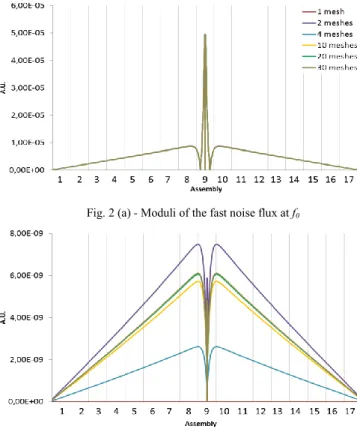
Next, we check the convergence of the vibration model when we increase the refinement of the meshing in the four perturbed regions. To do this, we will compare six different meshings in a one-dimensional core in two-groups (fast and thermal) with vacuum boundaries. The core is composed by 17 assemblies themselves composed by 17 fuel cells. We choose to perturb the central fuel pin of this symmetric geometry with a vibration frequency f0 =
1 Hz and a particularly small amplitude of 0.018 cm (the fuel pin size is 1.08 cm and the inter-pin size is 0.36 cm so one cell size is 1.44 cm). Here we simply use the traditional linearization method of section II.A in diffusion theory and we only show the results for the modulus of the fast noise flux. Figure 2 illustrates the results.
Fig. 2 (a) - Moduli of the fast noise flux at f0
Fig. 2(b) - Moduli of the fast noise flux at 7f0
Fig. 2 - Convergence of the vibration model in function of the mesh refinement
We find that the vibration model converges if we increase the refinement of the meshing. We find the same convergence with the thermal noise flux. Note that the higher the harmonic order is the more the mesh has to be refined.
IV. ANALYSIS OF A FUEL PIN VIBRATION IN A ONE-DIMENSIONAL CORE
In this section, we present the results of a fuel pin vibration in the one-dimension diffusion theory with four-groups (and six precursors four-groups). Note that the fluctuations of the diffusion coefficients are disregarded. We also neglect the term 𝑣𝑔1 𝜕𝑡 𝐽𝑔 (with 𝐽𝑔 the scalar
current of group 𝑔). Groups 1 and 2 are fast groups and groups 3 and 4 are thermal groups. We work with the same core of section III.B. but we choose to perturb the central fuel pin of the third assembly with an amplitude of 0.09 cm (with 20 meshes per perturbed region). We use also a frequency f0 =1 Hz, a common frequency for a fuel pin
vibration. The fuel pin moves to the right side during the interval [0,𝑇0
2] and to the left side during the interval
[𝑇0
2, 𝑇0].
Firstly, we quickly present the global and local components of the noise flux in order to understand more easily the following results. After that, we compare the noise fluxes in the frequency domain and the total fluxes in the time domain between three solution methods:
the traditional method noted 𝛷𝑇 with the steady-state flux 𝛷0,𝑇 (section II.A, notation T for “Traditional”); the method with 𝐵0,𝑁𝐹 noted 𝛷𝑁𝐹 with the steady-state flux 𝛷0,𝑁𝐹 (section II.B, notation NF for “New
Flux”);
the exact solution (in diffusion theory) noted 𝛷𝑅
with the steady-state flux 𝛷0,𝑅 (section II.C, we
choose a large convolution amplitude of 15, notation
R for “Reference”);
To simplify the analysis, we present the results for groups 1 and 4. Group 2 results (resp. 3) are equivalents to group 1 results (resp. 4). For all calculations, the maximal relative errors of the noise flux and the fission sources between two iterations are 10−6.
IV.A. General proprieties of the global and local components
The neutron noise in a nuclear reactor can be separated into two components: a global and a local components [5], [6]. The local component is rapidly changing along the axis and is of a high frequency nature while the global component is slowly varying in space and is confined to low frequencies. The local component corresponds to a rapid relaxation in space and so exists only in the vicinity of the perturbation, and the global component follows a much lower relaxation and impacts the entire core. In the time domain, the noise flux is always composed by these two components but the balance between them can be different in function of the energy group, the vibration frequency or the core size. Here we have some important proprieties of these components:
the global component dominates in low frequencies while the local in high frequencies;
the global component dominates in small or tightly coupled core while the local in large or few coupled core;
the local component affects more the thermal noise flux than the fast noise flux;
the global component can be described by the point reactor model in small core, not in large core;
the global component should be more affected by the
high order terms of the noise flux than the local component.
IV.B. The noise flux harmonics in the frequency domain
Figure 3 compares the moduli of harmonics 1, 2, 3 and 4 of the exact noise flux in groups 1 and 4. We use 20 meshes per perturbed region so we have a good convergence of the noise source for all these harmonics. We remark that harmonics 1 and 2 dominate and that the contribution of harmonics 3 and 4 (and therefore of the higher-order harmonics) can be neglected. We have obtained similar results with the other methods. Thus, the more important harmonics of the noise source are at f0 and
2f0.
Fig. 3(a) - Moduli in group 1
Fig. 3(b) - Moduli in group 4 (zoom in on the third assembly)
Fig. 3 - Comparison between the moduli of harmonics 1, 2, 3 and 4 of the exact noise flux in groups 1 and 4
This observation can be explained by the fact that, in each one of the four regions (see Fig. 1(a)), 𝛿Σ(𝑟, 𝜔) does not change of sign for 𝜔0 and 2𝜔0 whereas it changes of
sign for all others harmonics (see Fig.4). Thus, for harmonics greater than two, the noise source changes of sign within each perturbed region and, as shown in Fig. 3, the final effect is a very small noise flux. Consequently, we will only detail the two first components of the noise flux.
Fig. 4 - 𝛿Σ in function of mesh and frequency for region 4 with 20 meshes.
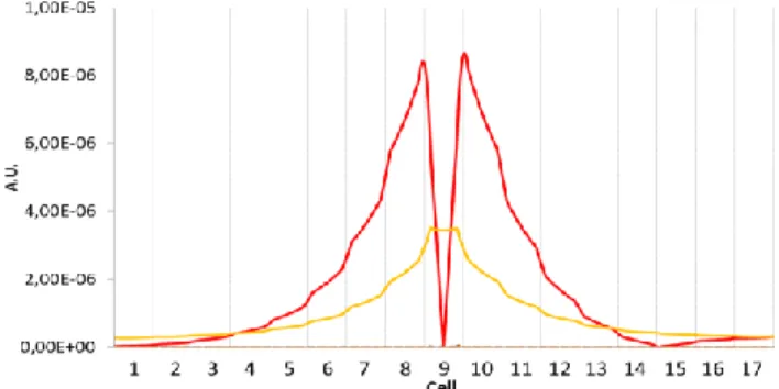
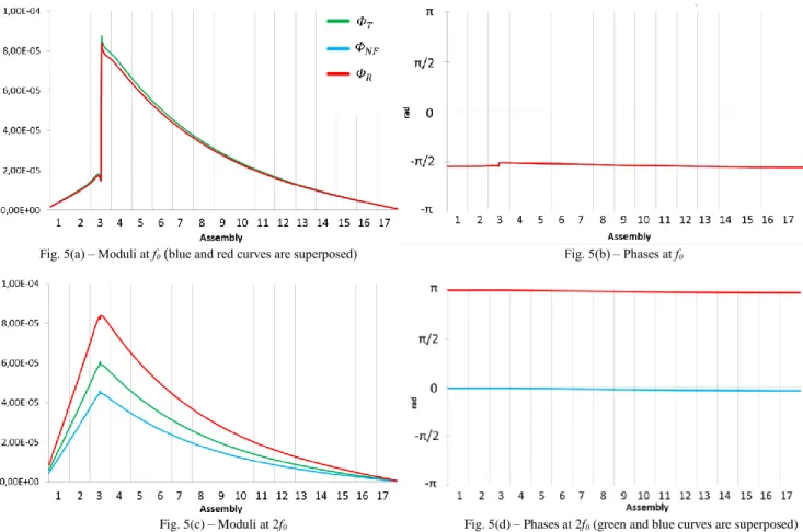
Figures 5 and 6 compare the moduli and the phases of the first and second harmonics of the noise flux in groups 1 and 4 for the three methods. Note that we have zoom in on the third assembly for the moduli of group 4. At f0, the three
methods are very close to each other while at 2f0 we
observe some significant differences between them. Let us begin by analyzing the modulus at f0. For group
1, we have a global component, which has a slow variation in space, and a local component in the vicinity of the vibration in the third assembly. Its phase is constant in the entire core (around -π/2). For group 4, the local component strongly dominates in the vicinity of the vibration with several rough phase changes. Its phase is constant far from the perturbation (around -π/2). Compared to group 1, the global component far from the vibration seems to be negligible and crushed by the amplitude of the local
component. At 2f0, we can observe similar behaviors but
with a phase around 0 for 𝛷𝑇 and 𝛷𝑁𝐹 and around +π for
𝛷𝑅.
We can conclude that in the vicinity of the perturbation the global and local component for f0 and 2f0
are visible for the fast group while only the local component is visible for the thermal one. Far from the perturbation, only the global component exists for all groups but its amplitude is greater for the fast group than for the thermal group. Moreover, we have a phase shift of ±π/2 depending on the method between these two harmonics.
Next, we compare the three methods. At f0, 𝛷𝑁𝐹 is
closer to the exact solution than 𝛷𝑇while at 2f0 𝛷𝑇 is closer
to the exact solution than 𝛷𝑁𝐹. But as the first harmonic is
more important that the second harmonic (not always but especially in group 4), we have a balance between these
differences and we cannot say that 𝛷𝑇 is closer to the exact
solution than 𝛷𝑁𝐹, or conversely.
The phase shift of π between 𝛷𝑇 or 𝛷𝑁𝐹 and the exact
solution can be explained by the importance of the convolution term [𝛿𝐵𝑅∗ 𝛿Φ𝑅](𝑟, 2𝜔0) especially the term
𝛿𝐵𝑅(𝜔0)𝛿Φ𝑅(𝜔0) which is the more important term of the
convolution.
We note that the second harmonic affects more the fast group than the thermal one and so affects more the global than the local component. We also verify that the global component cannot be described by the point reactor model in a large core and that the local component affects more the thermal noise flux than the fast noise flux.
Let us precise that some of our observations about the global and local components and the first and second harmonics are in agreement with [7] but in our case the second harmonic is not negligible.
Fig. 5(a) – Moduli at f0(blue and red curves are superposed) Fig. 5(b) – Phases at f0
Fig. 5(c) – Moduli at 2f0 Fig. 5(d) – Phases at 2f0 (green and blue curves are superposed)
IV.C. The total flux in the time domain
The total flux in the time domain is here defined by the steady-state flux and the first and second harmonics of the noise flux:
𝛷(𝑟, 𝑡) ≈ 𝛷0(𝑟) +|𝛿𝛷|(𝑟,𝜔𝜋 0)cos(𝜔0𝑡 + 𝜑(𝑟, 𝜔0))
+ |𝛿𝛷|(𝑟,2𝜔0)
𝜋 cos(2𝜔0𝑡 + 𝜑(𝑟, 2𝜔0)), (28)
where 𝛷 is the scalar flux, |𝛿𝛷| is the modulus of the noise scalar flux and
𝜑
its phase.The eigenvalues of the three steady states are 𝑘𝑇=1.000016, 𝑘𝑁𝐹=0.9999347 and 𝑘𝑅=0.9999401. These
eigenvalues are very close to each other. Figure 7 presents the steady-state fluxes in groups 1 and 4. We remark that the steady-state operator 𝐵0,𝑁𝐹 seems to be a good
approximation of the exact steady-state operator.
Figures 8 and 9 present the total fluxes of groups 1 and 4 in the time domain at 𝑡 = 𝑇0/4 i.e. when the fuel pin
vibration hits its maximal amplitude at the right side. Figures 8(a) and 9(a) show that, at this time and at the right side of the perturbation, the fast flux is greater than the steady-state fast flux and that the thermal flux is smaller than the steady-state thermal flux. We also remark that, as expected, the global component is more dominating in the fast group than in the thermal group while the local component dominates more in the thermal group than in the fast group. Moreover, Fig. 9(b) points out the rapid relaxation length of the local component.
Figures 10 and 11 show the temporal variations of the noise flux in a position 𝑟𝑎 close to the perturbation (see
Fig. 8(a)) and a position 𝑟𝑏 far from the perturbation (close
to the core center).
Fig. 6(a) – Moduli at f0 (zoom in on the third assembly) Fig. 6(b) – Phases at f0
Fig. 6(c) – Moduli at 2f0 (zoom in on the third assembly) Fig. 6(d) – Phases at 2f0 (green and blue curves are superposed)
For the position 𝑟𝑎 close to the vibration, in group 1,
the second harmonic is clearly not negligible compared to the first harmonic. In group 4, the second harmonic is less visible. Moreover, we note the differences between 𝛷𝑁𝐹 and the exact solution 𝛷𝑅 are more visible in group 1
than in group 4. But we saw that, close to the vibration, the global and local component are visible for the fast group 1 while only the local component dominates for the thermal group 4. So this observation is coherent with the fact that the global component should be more affected by the high order terms of the noise flux than the local component. It is also coherent with the fact that the second harmonic of the
noise flux impacts more the global than the local component.
For the position 𝑟𝑏 far from the perturbation where the
global component dominates for all groups, the balance between harmonic 1 and 2 is the same for groups 1 and 4 but the amplitudes of the total flux variations are really different. In group 1, the maximal amplitude is around 2.10−5 while in group 4 is around 7.10−8. As we saw
previously, the amplitude of the global component is clearly more important for the fast group than for the thermal group.
Fig. 7(a) – Group 1 Fig. 7(b) – Group 4 (zoom in on the third assembly)
Fig.7 – Steady-state fluxes in groups 1 and 4 (blue and green curves are superposed)
Fig. 8(a) - The vibrated fuel pin (green regions delimit the perturbed regions) Fig. 8(b) - The third assembly
Fig. 8 - Total fluxes in group 1 at 𝑡 =𝑇0 4
Fig. 9(a) - The vibrated fuel pin (green regions delimit the perturbed regions) Fig. 9(b) - The third assembly
Fig. 9 - Total fluxes in group 4 at 𝑡 =𝑇40
Fig. 10(a) – Total fluxes at 𝑟𝑎 Fig. 10(b) – Total fluxes at 𝑟𝑏
Fig. 10 – Total fluxes in group 1 at 𝑟𝑎 and 𝑟𝑏 in function of time (same legend of previous figures)
Fig. 11(a) – Total fluxes at 𝑟𝑎 Fig. 11(b) – Total fluxes at 𝑟𝑏
V. CONCLUSIONS
A one-dimension vibration model has been developed. This source perturbation excites all multiples of the vibration frequency f0. The more important harmonics of
this noise source are at f0 and 2f0. We noted that the
modulus of this second harmonic is more important and closer to the first harmonic for the global than the local component of the noise flux and for fast groups than for thermal groups.
We introduced a new method in order to improve the traditional linearization method, which is not theoretically justified in case of vibration perturbation. Because in a vibration perturbation the mean values of the perturbed cross-sections are not zero, in this new method we use a new steady-state operator which is the time-average of the kinetic operator and not the initial critical operator as in the traditional method.
We compared this new method with the traditional method and with the exact solution of the non-linearized, fully-coupled noise equations in diffusion theory and for four energy groups. We concluded that the second harmonic of the noise flux is not negligible, should be taken into account and affects especially the global component of the noise flux. We also noted that the differences between all methods are more important at 2f0
than f0. Moreover, the new method is based on a
steady-state flux closer to the steady-steady-state flux of the exact solution compared to the traditional steady-state flux. We also verified that the global (resp. local) component of the noise flux dominates in fast (resp. thermal) group, that it cannot be described by the point reactor model in a large system and more especially that it is more affected by the high order terms of the noise flux than the local component.
Thanks to many other calculations not presented here with different vibration amplitudes and different system sizes, we observed that the modulus of the second harmonic is more important and closer to the first harmonic for a large system than for a small system and for a large vibration amplitude than for a small vibration amplitude. Moreover, the high order terms are logically more important in case of a large vibration amplitude compared to a small vibration amplitude and they are also more important for a small system than for a large system. In this paper, we use the classical assumptions of noise diffusion theory i.e. the fluctuations of the diffusion coefficients and the term 𝑣𝑔1 𝜕𝑡 𝐽𝑔 are neglected. Future
work will investigate these assumptions and will compare transport and diffusion results in case of fuel pin vibration in two-dimensional systems.
Moreover, a new method, which should improve traditional linear noise theory, will be presented. This new technique respects also the linear theory but improves the noise source term by using a more physically realistic steady-state flux.
ACKNOWLEDGMENTS
The authors wish to thank Professor I. Pázsit for helpful discussions. We gratefully acknowledge AREVA and EDF for their long term partnership and their support.
REFERENCES
1. I. Pázsit and C. Demazière, “Noise Techniques in Nuclear Systems”, Handbook of Nuclear Engineering, Ed. Cacuci, D. G., Vol. 3, Chapter 2, Springer Verlag, (2010).
2. I. Pázsit, “The Linearization of Vibration-Induced Noise”, Ann. Nucl. Energy, 11, 441-454 (1984). 3. I. Pázsit, J. Karlsson, “On the perturbative calculation
of the vibration noise by strong absorbers”, Ann. Nucl.
Energy, 24, 449-466 (1997).
4. A.M. Weinberg, H.C. Schweinler, “Theory of Oscillating Absorber in a Chain Reactor”, The
Physical Review, 74, 8, 851-863 (1948).
5. K. Behringuer, G. Kosály, Lj. Kostic, “Theoretical Investigation of Local and Global Components of the Neutron-Noise Field in a Boiling Water Reactor”, Ann.
Nucl. Energy, 63, 306-318 (1977).
6. V. Dykin, I. Pázsit, “The role of the eigenvalue separation in reactor dynamics and neutron noise theory”, PHYSOR 2014 (2014).
7. I. Pázsit, 1977. “Investigation of the Space-dependent Noise Induced by a Vibrating Absorber”, Atomkernenergie (ATKE), 30, 29 (1977).