HAL Id: cea-01326375
https://hal-cea.archives-ouvertes.fr/cea-01326375
Submitted on 3 Jun 2016
HAL is a multi-disciplinary open access
archive for the deposit and dissemination of
sci-entific research documents, whether they are
pub-lished or not. The documents may come from
teaching and research institutions in France or
abroad, or from public or private research centers.
L’archive ouverte pluridisciplinaire HAL, est
destinée au dépôt et à la diffusion de documents
scientifiques de niveau recherche, publiés ou non,
émanant des établissements d’enseignement et de
recherche français ou étrangers, des laboratoires
publics ou privés.
Event-plane correlators
Rajeev S. Bhalerao, Jean-Yves Ollitrault, Subrata Pal
To cite this version:
Rajeev S. Bhalerao, Jean-Yves Ollitrault, Subrata Pal. Event-plane correlators. Physical Review C,
American Physical Society, 2013, 88 (2), pp.4909. �10.1103/PhysRevC.88.024909�. �cea-01326375�
arXiv:1307.0980v2 [nucl-th] 22 Aug 2013
Rajeev S. Bhalerao,1 Jean-Yves Ollitrault,2 and Subrata Pal3
1
Department of Theoretical Physics, Tata Institute of Fundamental Research, Homi Bhabha Road, Mumbai 400005, India
2
CNRS, URA2306, IPhT, Institut de physique theorique de Saclay, F-91191 Gif-sur-Yvette, France
3
Department of Nuclear and Atomic Physics, Tata Institute of Fundamental Research, Homi Bhabha Road, Mumbai 400005, India
(Dated: August 23, 2013)
Correlators between event planes of different harmonics in relativistic heavy-ion collisions have the potential to provide crucial information on the initial state of the matter formed in these col-lisions. We present a new procedure for analyzing such correlators, which is less demanding in terms of detector acceptance than the one used recently by the ATLAS collaboration to measure various two-plane and three-plane correlators in Pb-Pb collisions at LHC. It can also be used un-ambiguously for quantitative comparison between theory and data. We use this procedure to carry out realistic simulations within the transport model AMPT. Our theoretical results are in excellent agreement with the ATLAS data, in contrast with previous hydrodynamic calculations which only achieved qualitative agreement. We present predictions for new correlators, in particular four-plane correlators, which can easily be analyzed with our new method.
PACS numbers: 25.75.Ld, 24.10.Nz
Introduction.−High-energy heavy-ion collision exper-iments at the Relativistic Heavy-Ion Collider (RHIC), BNL and the Large Hadron Collider (LHC), CERN have firmly established the formation of strongly interacting matter which exhibits a strong collective flow [1–3]. This not only suggests that the matter formed is close to lo-cal thermal equilibrium but also provides a window to the initial state of the fireball immediately after the col-lision. Collective flow in the plane transverse to the beam axis is typically measured in terms of two-particle angu-lar correlations [4–7] and its small anisotropies captured in its Fourier harmonics [8–11]. Recently, a new tool, namely correlations among event planes corresponding to different harmonics [12–14], is emerging with a promise to throw additional light on the initial-state phenomena. Pair correlations (i.e., the single-particle anisotropic flow vnextracted from two-particle correlations) are
rea-sonably well understood [8]. Event-plane correlators rep-resent higher-order correlations, involving at least three particles. Such higher-order correlations thus open a new direction in heavy-ion physics, much in the same way as studies of non-Gaussian fluctuations [15] in the early Uni-verse. They bring in a large number of new observables which provide new, detailed insight into the hydrody-namic response and on the initial stage, and will signifi-cantly improve our understanding of heavy-ion collisions. The ATLAS collaboration [14] has recently released preliminary measurements of eight two-plane correlators (e.g., the correlation between the second and fourth har-monics) and six three-plane correlators (e.g., the mixed correlation between second, third and fifth harmonics) in Pb-Pb collisions at √sN N = 2.76 TeV, as a function
of the centrality of the collision. These correlators are qualitatively understood within event-by-event hydrody-namics [16] and provide new insight [17] into the
inter-play between the linear and nonlinear [18] hydrodynamic response [19, 20] to the initial density profile.
The ATLAS analysis is very demanding in terms of detector acceptance: each event plane is determined in a separate pseudorapidity window; windows must be pair-wise separated by gaps in order to suppress nonflow cor-relations; finally, each window must be wide enough to achieve a significant resolution in every Fourier harmonic up to order six.
In this article, we show that the analysis can be done more simply, and that even three- and four-plane corre-lators can be safely analyzed with just two symmetric pseudorapidity windows, in the same way as two-plane correlators. The analysis can thus be performed by other experiments with smaller detector acceptance. We also explain in detail how to generalize the scalar-product method used earlier for two-particle flow analysis [21], to mixed correlations, so as to eliminate the ambiguity brought about by the event-plane method [22].
We carry out realistic simulations within a multiphase transport (AMPT) model [23]. Results are for the first time in quantitative agreement with the ATLAS mea-surements. In addition, we present predictions for several new correlators, in particular four-plane correlators.
M ethod.−The azimuthal distribution of outgoing par-ticles is decomposed in Fourier harmonics in each col-lision event. The flow vector in harmonic n is defined as [24], Qn= |Qn|einΨn≡ 1 N X j einφj, (1)
where we have used a complex notation and the sum runs over N particles seen in a reference detector, and φj are
their azimuthal angles. Ψn is dubbed the event-plane
2
The idea of ATLAS [14] is to measure angular cor-relations between different harmonics, that is, between Ψn and Ψm with n 6= m. We take as an illustration
the correlation between the 2nd and 4th harmonic planes Ψ2 and Ψ4. In order to ensure that the measured
cor-relation is due to collective flow [25], one measures Ψ4
and Ψ2 in different parts of the detector (“subevents”)
A and B separated by a gap in pseudorapidity (i.e., po-lar angle). The simplest observable one can think of is hcos(4(Ψ4A− Ψ2B))i. Since, however, Ψ4Aand Ψ2Bhave
statistical fluctuations due to the finite number of par-ticles in each subevent, one corrects for these statistical fluctuations by a so-called “resolution” correction [24]. The quantity measured by ATLAS can be written ex-plicitly as hcos 4(Φ2− Φ4)i ≡ D Q22A |Q2 2A| Q∗ 4B |Q4B| E rD Q 4A |Q4A| Q∗ 4B |Q4B| ErD Q2 2A |Q2 2A| Q∗2 2B |Q2 2B| E, (2) where we have used the same notation as ATLAS on the left-hand side, and angular brackets on the right-hand side denote the real part of the average over events. The numerator is hcos(4(Ψ4A− Ψ2B))i and the denominator
is the resolution correction [26].
As shown in [22], Eq. (2) represents an ambiguous mea-surement, in the sense that the denominator does not properly correct for the resolution when flow fluctuations are present [27, 28]. If one repeats the analysis with a lower resolution (typically, smaller subevents A and B), both the numerator and the denominator decrease, but the denominator decreases faster than the numera-tor, resulting in an increase of the signal. The difference between the low-resolution limit and the high-resolution limit can be as large as 50% for the above correlation [22]. In practice, experimental values are likely to be close to the low-resolution limit, due to the poor resolution in higher harmonics. However, the value calculated in hy-drodynamics [16, 17] is the high-resolution limit, so that a quantitative comparison between theory and data is impossible at present.
These ambiguities can easily be removed. One simply replaces Eq. (2) with [22]:
c{2, 2, −4} ≡ Q2 2AQ∗4B p hQ4AQ∗4Bi p hQ2 2AQ∗22Bi , (3)
where the notation on the left-hand side [12] expresses that the numerator involves two particles in harmonic 2 (i.e., two factors of Q2) and one particle in harmonic −4
(one factor of Q∗
4). Equations (2) and (3) are referred
to as “event-plane” (EP) method and “scalar product” (SP) method [21], respectively.
The only difference is that the scalar-product method retains the information on the length of Qn. We now
explain why this simple modification ensures that the
right-hand side of Eq. (3) is a well-behaved flow observ-able, unlike (2). The flow picture is a model in which particles are emitted randomly and independently ac-cording to some underlying probability distribution in each event [29]. The azimuthal probability distribution is written as P (φ) = 1 2π +∞ X n=−∞ vneinΦne−inφ, (4)
where vn is the anisotropic flow in harmonic n and Φn
the corresponding reference direction [29, 30] (we use the convention v0 = 1). The average over events can be
performed in two steps, by first averaging over events with the same P (φ), then averaging over values of vn
and Φn [22]:
h. . .i =Dh. . .i|vn
E
. (5)
Equations (1) and (4) yield hQni|vn= vne
inΦn. Now, the
crucial point is that Eq. (3) only involves products of Qn
vectors. Since particles are emitted independently, the expectation value of a product is the product of expec-tation values, therefore
Q22AQ∗4B |vn = (v2) 2v 4e4i(Φ2−Φ4), hQ4AQ∗4Bi|vn = (v4) 2, Q22AQ∗22B |vn = (v2) 4. (6)
These equations show that each of the quantities entering Eq. (3) is a well-defined flow observable.
We now explain why we choose to measure the partic-ular combination in the right-hand side of Eq. (3). The three observables in Eq. (6) are sensitive to the magni-tudes of v2 and v4. By taking the ratio in Eq. (3), one
singles out the angular correlation, in the sense that if one multiplies v2and/or v4by a constant, the right-hand side
of Eq. (3) is unchanged. We therefore call this quantity an “event-plane correlator”, even though it involves the statistics of v2 and v4, and not just the underlying
direc-tions Φ2 and Φ4. Equations (5) and (6) predict that the
right-hand side of Eq. (3) should lie between -1 and 1 by the Cauchy-Schwarz inequality [31].
It can be shown that Eq. (3) coincides with Eq. (2) in the limit of low resolution [22] but, as shown above, it is independent of the experimental resolution, unlike Eq. (2), and thus yields an unambiguous measurement. The only price to pay for the loss of ambiguity is a larger statistical error.
Note that the two-plane correlator defined by Eq. (3) actually involves a three-particle correlation [32]. This is easily seen by inserting the definition of Qn, Eq. (1), into
the numerator of Eq. (3). One obtains
Q22AQ∗4B = 1 N2 ANB X j∈A X k∈A X l∈B
that is, an average of e2iφj+2iφk−4iφl over all triplets of
particles.
In order to guarantee that correlations are dominated by flow, one should in principle implement pseudorapid-ity gaps between all particles. In Eq. (7), however, there is no pseudorapidity gap between j and k, and there are even self-correlation terms j = k. Therefore, the pro-cedure followed by ATLAS does not, strictly speaking, avoid self correlations.
We now explain why the contribution of nonflow cor-relations and self-corcor-relations to Eq. (7) is small, thus justifying the procedure. It is generally accepted that long-range correlations are dominated by flow [25] or, equivalently, that nonflow correlations are short range (with the exception of global momentum conservation, which only contributes to the first Fourier harmonic [33]). Short-range correlations are effects which correlate a par-ticle with its neighbors with some probability, so that such correlations are typically a small fraction of self-correlations [34]. We thus evaluate the contribution of self-correlations to Eq. (7). The thumb rule is that each factor of einφ gives a contribution of order v
n. Thus the
right-hand side of Eq. (7) is typically of order v4(v2)2.
Self-correlations terms j = k give a contribution of or-der (v4)2/NA. Since v4 ∼ (v2)2 [35], the relative
magni-tude of self-correlations is of order 1/NA, which is small.
Note that self-correlations can also be removed explicitly if particles are seen individually [36].
The discussion can be repeated for the three-plane cor-relation between harmonics 2, 3 and 5. ATLAS measures the three harmonics in three separate subevents A, B and C. We now show how the analysis can be done with just two subevents A and B. In close analogy with (3), we define c{2, 3, −5} ≡ hQ2AQ3AQ ∗ 5Bi p hQ2AQ∗2Bi hQ3AQ∗3Bi hQ5AQ∗5Bi , (8) where the numerator is a mixed correlation between har-monics 2, 3 and 5, and the denominator the correspond-ing resolution correction in each harmonic. We now ex-plain why nonflow effects are small, even though the 2nd and 3rd harmonic are measured in the same subevent A. We decompose the numerator of Eq. (8) as
Q2AQ3AQ∗5B = 1 N2 ANB X j∈A X k∈A X l∈B
e2iφj+3iφk−5iφl. (9)
Flow typically gives a contribution of order v2v3v5. Self
correlations are terms j = k, which give a contribution of order (v5)2/NA. Since v5∼ v2v3[20], the relative order of
self-correlations (and therefore of nonflow correlations) is 1/NA, exactly as for the two-plane correlator c{2, 2, −4}
considered above. Therefore this three-plane correlator does not require three separate subevents.
This discussion can be easily generalized to all other correlations. The general prescription for the pseudo-rapidity gap is that all the positive harmonics (i.e., all
factors of Qn) should go on one side (e.g., A), and all
negative harmonics (all factors of Q∗
n) on the other side
(B). In this case, self-correlation terms are of relative order vn+p/(N vnvp) ∼ 1/N, and nonflow effects can be
safely neglected. Therefore all three-plane correlators measured by ATLAS can be analyzed with a single pseu-dorapidity gap. The analysis can be extended to four-plane correlators and higher.
If kn denotes the number of particles in harmonic n,
the correlator can be generally written as
c{· · · , n, n, n | {z } kn , · · · } ≡ * Y n>0 (QnA)kn Y n<0 (QnB)kn + rY n (QnA)kn(Q∗nB)kn . (10) Azimuthal symmetry requiresPnnkn = 0 [12]. As an
example, we write explicitly the formula for the lowest-order four-plane correlator [37]:
c{2, −3, −4, 5} ≡
hQ2AQ5AQ∗3BQ∗4Bi
p
hQ2AQ∗2Bi hQ3AQ∗3Bi hQ4AQ∗4Bi hQ5AQ∗5Bi
, (11)
for which we give the first quantitative prediction below. While two-plane correlations thus defined all lie between −1 and +1 by the Cauchy-Schwarz inequality, there is no such restriction for three- and four-plane correlators. We shall give below an example of a four-plane correlator exceeding unity in AMPT calculations.
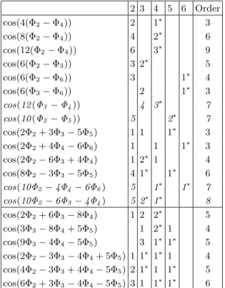
Table I lists the fourteen correlations studied by AT-LAS, as well as six additional correlations predicted for the first time in this paper. For clarity, each correlation is written using the same notation as ATLAS (left col-umn). The next columns list the number of particles in harmonics 2 to 6. In our notation, the first two corre-lators are written as c{2, 2, −4} and c{2, 2, 2, 2, −4, −4}, respectively. Table I shows that the two-plane correlators measured by ATLAS actually involve three to nine par-ticles —never just two— yet they can safely be analyzed with a single pseudorapidity gap, and so can three- and four-plane correlators. Table I also shows that more par-ticles are allowed in lower harmonics where the resolution is better.
Results.−Calculations are performed using the AMPT model [23] that consists of four main components: ini-tial conditions based on Glauber model, parton cascade, hadronization, and hadron scattering. We employ the version of AMPT with string melting and parton coales-cence for hadronization that describes better the collec-tive behavior in heavy-ion collisions at RHIC and LHC [23, 38, 39]. Flow is mostly produced in this model by elastic scatterings in the partonic phase. In addition, the model contains resonance decays and thus includes non-trivial nonflow effects. The implementation used here is the same as in Ref. [39], and uses initial conditions from
4
TABLE I. List of two-, three- and four-plane correlators. For each correlator, the number in column n indicates the number knof particles involved in harmonic n. Asterisks indicate that
the particles actually go into harmonic −n instead of n. The last column is the order of the correlation, i.e., the number of particles Pnkn. The first fourteen lines correspond to
the correlators measured by ATLAS [14] (correlators in italics are not studied in this paper), and the next six lines to new correlators predicted in this paper.
2 3 4 5 6 Order cos(4(Φ2− Φ4)) 2 1∗ 3 cos(8(Φ2− Φ4)) 4 2∗ 6 cos(12(Φ2− Φ4)) 6 3∗ 9 cos(6(Φ2− Φ3)) 3 2∗ 5 cos(6(Φ2− Φ6)) 3 1∗ 4 cos(6(Φ3− Φ6)) 2 1∗ 3 cos(12 (Φ3 − Φ4)) 4 3∗ 7 cos(10 (Φ2 − Φ5)) 5 2∗ 7 cos(2Φ2+ 3Φ3− 5Φ5) 1 1 1∗ 3 cos(2Φ2+ 4Φ4− 6Φ6) 1 1 1∗ 3 cos(2Φ2− 6Φ3+ 4Φ4) 1 2∗ 1 4 cos(8Φ2− 3Φ3− 5Φ5) 4 1∗ 1∗ 6 cos(10Φ2 − 4Φ4 − 6Φ6) 5 1∗ 1∗ 7 cos(10Φ2 − 6Φ3 − 4Φ4) 5 2∗ 1∗ 8 cos(2Φ2+ 6Φ3− 8Φ4) 1 2 2∗ 5 cos(3Φ3− 8Φ4+ 5Φ5) 1 2∗ 1 4 cos(9Φ3− 4Φ4− 5Φ5) 3 1∗ 1∗ 5 cos(2Φ2− 3Φ3− 4Φ4+ 5Φ5) 1 1∗ 1∗ 1 4 cos(4Φ2− 3Φ3+ 4Φ4− 5Φ5) 2 1∗ 1 1∗ 5 cos(6Φ2+ 3Φ3− 4Φ4− 5Φ5) 3 1 1∗ 1∗ 6
the HIJING 2.0 model [40]. We have checked that it re-produces LHC data for anisotropic flow (v2 to v6) at all
centralities [38, 39, 41].
AMPT simulation events can be analyzed with the same methods as actual experimental events. However, in AMPT, the energy-momentum information of all final-state particles in an event is available, whereas ATLAS only detects charged particles with pT > 0.5 GeV/c. We,
therefore, use all particles in our analysis which results in a better resolution.
As explained above, our analysis of event-plane cor-relations uses two subevents A and B, for which we use two symmetric pseudorapidity intervals −4.8 < η < −0.4 and 0.4 < η < 4.8, very similar to those by ATLAS for two-plane correlators. Each correlator is analyzed us-ing both scalar-product (SP) method (Eq. (10)) and the event-plane (EP) method (in which one replaces Qn by
Qn/|Qn| everywhere in Eq. (10)). Recall that the EP
result typically increases (in absolute magnitude) as the resolution decreases, while the SP result is the limit of low resolution. We thus expect that SP is larger than EP. If the model is valid, the experimental result (which is obtained with the EP method, but a lower resolution)
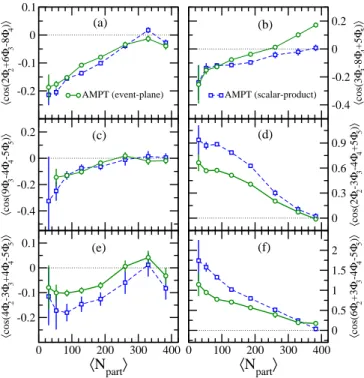
0 100 200 300 400 〈Npart〉 0 0.2 0.4 0.6 〈 cos 6( Φ2 -Φ6 ) 〉 0 100 200 300 400 〈Npart〉 0 0.2 0.4 0.6 〈 cos 6( Φ3 -Φ6 ) 〉 0 0.02 0.04 〈 cos 6( Φ2 -Φ3 ) 〉 0 0.2 0.4 0.6 0.8 〈 cos 12( Φ2 -Φ4 ) 〉 AMPT (scalar-product) 0 0.2 0.4 0.6 0.8 1 〈 cos 4( Φ2 -Φ4 ) 〉 ATLAS (event-plane) 0 0.2 0.4 0.6 0.8 1 〈 cos 8( Φ2 -Φ4 ) 〉 AMPT (event-plane) (e) (b) (d) (a) (c) (f)
FIG. 1. (Color online) Two-plane correlators in the event-plane (open circles) and scalar-product (open squares) meth-ods as a function of the number of participants in Pb-Pb collisions at√sN N = 2.76 TeV in the AMPT model as
com-pared to the ATLAS data [14] for the event-plane method (solid circles). We keep the notation of ATLAS hcos(· · · )i for simplicity, even though the measured quantities are not pure event-plane correlators.
should lie somewhere between the two AMPT predic-tions.
Figure 1 displays the results for two-plane correlators. Figures 1(a) and 1(b), which have the smallest error bars, show that the SP method gives larger results than the EP method, as expected [22]. The difference is in the range (10-15)%. EP results are in perfect agreement with data. This is in contrast with EP calculations in hydrodynam-ics, which are clearly below data [16, 17].
0 100 200 300 400 〈Npart〉 -0.3 -0.2 -0.1 0 〈 cos(2 Φ2 + 4 Φ4 -6 Φ3 ) 〉 AMPT (scalar-product) 0 100 200 300 400 〈Npart〉 -0.3 -0.2 -0.1 0 0.1 0.2 〈 cos(8 Φ2 -3 Φ3 -5 Φ5 ) 〉 0 0.2 0.4 0.6 0.8 1 〈 cos(2 Φ2 + 3 Φ3 -5 Φ5 ) 〉 ATLAS (event-plane) 0 0.2 0.4 0.6 0.8 1 〈 cos(2 Φ2 + 4 Φ4 -6 Φ6 ) 〉 AMPT (event-plane) (b) (d) (a) (c)
FIG. 2. (Color online) Three-plane correlators. Legend is the same as in Fig. 1.
The correlations between the second and fourth har-monics (Figs. 1(a)−1(c)) and between the second and sixth harmonics (Fig. 1(e)) are understood [20] as coming mostly from the nonlinear hydrodynamic response, which couples v4 to (v2)2 and v6 to (v2)3. Their increase from
central to peripheral collisions is driven by the increase of v2 itself. Similarly, the correlations between harmonics 3
and 6 (Fig. 1(f)) is driven by the coupling between v6and
(v3)2: it decreases slightly as the collision becomes more
peripheral, in the same way as v3. Finally, the
correla-tion between harmonics 2 and 3 (Fig. 1(d)) is an order of magnitude smaller [13]. Our calculation agrees with data in all cases.
Figure 2 presents AMPT calculations for four three-plane correlators. Again, calculations are in per-fect agreement with data. c{2, 3, −5} and c{2, 4, −6} (Figs. 2(a) and 2(b)) are strong and driven by the nonlin-ear hydrodynamic response, in the same way as the cor-relation between harmonics 2 and 4. The c{2, 4, −3, −3} correlation has a more subtle origin [17], in the sense that it is not simply generated by the nonlinear response term v4∝ (v2)2, but it is also qualitatively reproduced by
event-by-event hydrodynamic calculations [16]. Finally, c{2, 2, 2, 2, −3, −5} is compatible with zero.
Figure 3 presents predictions for three new [37] three-plane correlators (Figs. 3(a)−3(c)), as well as three four-plane correlators (Figs. 3(d)−3(f)). The magnitude and centrality dependence of c{2, 3, 3, −4, −4} (Fig. 3(a)) are similar to those of c{2, 4, −3, −3} (Fig. 2(c)) and like-wise, this correlator is not simply generated by the
0 100 200 300 400 〈Npart〉 -0.2 -0.1 0 0.1 〈 cos(4 Φ2 -3 Φ3 +4 Φ4 -5 Φ5 ) 〉 0 100 200 300 400 〈Npart〉 0 0.5 1 1.5 2 〈 cos(6 Φ2 +3 Φ3 -4 Φ4 -5 Φ5 ) 〉 0 0.3 0.6 0.9 〈 cos(2 Φ2 -3 Φ3 -4 Φ4 +5 Φ5 ) 〉 -0.4 -0.2 0 0.2 〈 cos(9 Φ3 -4 Φ4 -5 Φ5 ) 〉 -0.2 -0.1 0 0.1 〈 cos(2 Φ2 +6 Φ3 -8 Φ4 ) 〉 AMPT (event-plane) -0.4 -0.2 0 0.2 〈 cos(3 Φ3 -8 Φ4 +5 Φ5 ) 〉 AMPT (scalar-product) (e) (b) (d) (a) (c) (f)
FIG. 3. (Color online) Predictions for new three- and four-plane correlators. Legend is the same as in Fig. 1.
v4 ∝ (v2)2 nonlinear response. Four-plane correlators
are much more sensitive to analysis details than two- or three-plane correlators: the difference between the scalar-product method and the event-plane method is roughly 50%. Two of these correlators (Figs. 3(d) and 3(f)) are large, which can again be understood as an effect of the nonlinear hydrodynamic response coupling v4 to (v2)2
and v5to v2v3[20]. Note that the last four-plane
correla-tor (Fig. 3(f)) is predicted to exceed unity when analyzed using the scalar-product method.
Conclusions.−We have argued that event-plane corre-lators in heavy-ion collisions can be analyzed with just two symmetric pseudorapidity windows. We have illus-trated the validity of our approach by analyzing events simulated within the AMPT model which reproduces for the first time the magnitude and centrality dependence of the measured correlators in Pb-Pb collisions at LHC. Much better agreement with data is achieved than in pre-vious hydrodynamic calculations using the event-plane method [16, 17]. This apparent discrepancy between data and hydrodynamic calculations may simply be due to the ambiguity of the event-plane method. It will then be re-solved once both experiment and theory switch from the event-plane method to the scalar-product method. We have presented predictions for new correlators, in partic-ular large four-plane correlators, which can be measured in forthcoming analyses. It would be interesting to study the correlators using the procedure presented here in the event-by-event hydrodynamical simulations to ascertain the sensitivity to initial-state models, namely the Monte-Carlo Glauber and the color-glass-condensate [42].
This work is funded by CEFIPRA under project 4404-2. JYO acknowledges support by the European Research Council under the Advanced Investigator Grant ERC-AD-267258.
[1] U. W. Heinz and R. Snellings, Ann. Rev. Nucl. Part. Sci. 63, 123 (2013).
[2] C. Gale, S. Jeon and B. Schenke, Int. J. Mod. Phys. A 28, 1340011 (2013).
[3] J. -Y. Ollitrault, Phys. Rev. D 46, 229 (1992).
[4] K. Adcox et al. [PHENIX Collaboration], Phys. Rev. Lett. 89, 212301 (2002).
[5] K. Aamodt et al. [ALICE Collaboration], Phys. Lett. B 708, 249 (2012).
[6] S. Chatrchyan et al. [CMS Collaboration], Eur. Phys. J. C 72, 2012 (2012).
[7] G. Aad et al. [ATLAS Collaboration], Phys. Rev. C 86, 014907 (2012).
[8] S. A. Voloshin, A. M. Poskanzer and R. Snellings, arXiv:0809.2949 [nucl-ex].
[9] B. Alver and G. Roland, Phys. Rev. C 81, 054905 (2010) [Erratum-ibid. C 82, 039903 (2010)].
[10] B. Alver et al. [PHOBOS Collaboration], Phys. Rev. Lett. 98, 242302 (2007).
6
[11] A. P. Mishra, R. K. Mohapatra, P. S. Saumia and A. M. Srivastava, Phys. Rev. C 77, 064902 (2008). [12] R. S. Bhalerao, M. Luzum and J. -Y. Ollitrault, Phys.
Rev. C 84, 034910 (2011).
[13] K. Aamodt et al. [ALICE Collaboration], Phys. Rev. Lett. 107, 032301 (2011).
[14] J. Jia [ATLAS Collaboration], Nucl. Phys. A 910-911, 276 (2013).
[15] A. P. S. Yadav and B. D. Wandelt, Phys. Rev. Lett. 100, 181301 (2008).
[16] Z. Qiu and U. Heinz, Phys. Lett. B 717, 261 (2012). [17] D. Teaney and L. Yan, Nucl. Phys. A 904-905, 365c
(2013).
[18] N. Borghini and J. -Y. Ollitrault, Phys. Lett. B 642, 227 (2006).
[19] F. G. Gardim, F. Grassi, M. Luzum and J. -Y. Ollitrault, Phys. Rev. C 85, 024908 (2012).
[20] D. Teaney and L. Yan, Phys. Rev. C 86, 044908 (2012). [21] C. Adler et al. [STAR Collaboration], Phys. Rev. C 66,
034904 (2002).
[22] M. Luzum and J. -Y. Ollitrault, Phys. Rev. C 87, 044907 (2013).
[23] Z. -W. Lin, C. M. Ko, B. -A. Li, B. Zhang and S. Pal, Phys. Rev. C 72, 064901 (2005).
[24] A. M. Poskanzer and S. A. Voloshin, Phys. Rev. C 58, 1671 (1998).
[25] M. Luzum, Phys. Lett. B 696, 499 (2011).
[26] In practice, one symmetrizes the numerator by
exchang-ing A and B to decrease the statistical error. [27] B. Alver et al., Phys. Rev. C 77, 014906 (2008). [28] J. -Y. Ollitrault, A. M. Poskanzer and S. A. Voloshin,
Phys. Rev. C 80, 014904 (2009).
[29] M. Luzum, J. Phys. G 38, 124026 (2011).
[30] S. Voloshin and Y. Zhang, Z. Phys. C 70, 665 (1996). [31] F. G. Gardim, F. Grassi, M. Luzum and J. -Y. Ollitrault,
Phys. Rev. C 87, 031901(R) (2013).
[32] N. Borghini, P. M. Dinh and J. -Y. Ollitrault, Phys. Rev. C 64, 054901 (2001).
[33] N. Borghini, P. M. Dinh and J. -Y. Ollitrault, Phys. Rev. C 62, 034902 (2000).
[34] R. S. Bhalerao, N. Borghini and J. Y. Ollitrault, Nucl. Phys. A 727, 373 (2003).
[35] A. Adare et al. [PHENIX Collaboration], Phys. Rev. Lett. 105, 062301 (2010).
[36] A. Bilandzic, R. Snellings and S. Voloshin, Phys. Rev. C 83, 044913 (2011).
[37] J. Jia and D. Teaney, arXiv:1205.3585 [nucl-ex]. [38] J. Xu and C. M. Ko, Phys. Rev. C 84, 044907 (2011). [39] S. Pal and M. Bleicher, Phys. Lett. B 709, 82 (2012); J.
Phys. Conf. Ser. 420, 012027 (2013).
[40] W. -T. Deng, X. -N. Wang and R. Xu, Phys. Rev. C 83, 014915 (2011).
[41] L. X. Han, G. L. Ma, Y. G. Ma, X. Z. Cai, J. H. Chen, S. Zhang and C. Zhong, Phys. Rev. C 84, 064907 (2011). [42] F. Gelis, E. Iancu, J. Jalilian-Marian, and R.