en fr

(1)

HAL Id: tel-01985286

https://tel.archives-ouvertes.fr/tel-01985286v2

Submitted on 11 Jun 2020

HAL is a multi-disciplinary open access archive for the deposit and dissemination of sci-entific research documents, whether they are pub-lished or not. The documents may come from teaching and research institutions in France or abroad, or from public or private research centers.

L’archive ouverte pluridisciplinaire HAL, est destinée au dépôt et à la diffusion de documents scientifiques de niveau recherche, publiés ou non, émanant des établissements d’enseignement et de recherche français ou étrangers, des laboratoires publics ou privés.

Alzheimer’s Disease

Jérémy Guillon

To cite this version:

Jérémy Guillon. Multilayer Approach to Brain Connectivity in Alzheimer’s Disease. Computer sci-ence. Sorbonne Université, 2018. English. �NNT : 2018SORUS305�. �tel-01985286v2�

(2)

Multilayer Approach

to Brain Connectivity

in Alzheimer’s Disease

J

ÉRÉMY

G

UILLON

(3)

(4)

Sorbonne Université

École Doctorale d’Informatique, de Télécommunication et d’Électronique (EDITE)

ARAMIS LAB à l’Institut du Cerveau et de la Moelle épinière (ICM)

Approche multi-niveaux de la

connectivité cérébrale dans la maladie

d’Alzheimer

MULTI-LAYER APPROACH TO BRAIN CONNECTIVITY IN AZLHEIMER’S DISEASE

JEREMY GUILLON

Thèse de doctorat d’informatique Dirigée par Fabrizio De Vico Fallani

Présentée et soutenue publiquement le 9 novembre 2018

Devant un jury composé de :

o M. Dimitri Van De Ville, Professeur (rapporteur) o M. Alex Arenas, Professeur (rapporteur)

o Mme. Raffaella Lara Migliaccio, Investigateur Principal

o M. Alexandre Gramfort, Enseignant-Chercheur o M. Fabrizio De Vico Fallani, Investigateur Principal

(5)

(6)

Table of

Remerciements

A MES ENCADRANTS.

J’aimerais avant tout remercier Fabrizio, encadrant de thèse pour qui il sera difficile de ne pas exagérer les éloges. Parfaitement équilibré ; ni trop présent ni trop absent ; ni trop compatissants ni trop exigeant, rassurant même pour respecter des deadlines impossibles... Perfectionniste à souhait, surtout lorsqu’il s’agit de figures d’articles, seules les couleurs pouvaient nous opposer !

Olivier, merci encore d’avoir fait suite à ma demande de stage dans l’équipe ARAMIS il y a maintenant 3 ans et demi, départ de cette aventure. Merci pour avoir été, avec Stanley,des chefs d’équipe exemplaires, toujours à l’écoute, toujours présents pour les pauses café avec des sujets de conversation toujours aussi passionnants, toujours prêts à entendre et écouter les critiques et les propositions.

AUX MEMBRES DE L’ECOLE DOCTORALE.

Je vous remercie d’avoir accepté ma candidature et de m’avoir donné l’opportunité de réaliser cette thèse.

À MESDAMES ET MESSIEURS LES MEMBRES DU JURY.

M. Dimitri Van de Ville, M. Alex Arenas, Mme. Rafaella Lara Migliaccio, M. Alexandre Gramfort, M. Lionel Tabourier, merci d’avoir accepté d’être membres du jury de ma thèse. Je suis très honoré de pouvoir présenter ces travaux devant vous et de pouvoir bénéficier de votre expertise.

(11)

Merci à ARAMIS LAB, le meilleur labo du monde, et à tous ceux que je ne pourrai pas citer individuellement qui sont, ou ont été et resteront, membres de l’équipe ! Et désolé à ceux que je citerai accompagnés d’un qualificatif trop bref pour être juste.

Merci à mes premiers compagnons de galère : Cata pour tous ces moments incroyavles, Jorge

pour avoir été là lors de la nuit la plus blanche de ma vie, Hao pour le doux son de ton beat box résonant dans les couloirs et Alexandre R. pour ta joie de vivre et ta motivation contagieuses !

A tous ceux des générations 3.0 et 4.0 : Alex le city boy, Igor le hipster, Maxime le grimpeur,

Manon la veggie, DJ Arnaud le woodfloor expert et Raphael l’aventurier, surfer-rider et bon dernier !

Au club des filles italiennes : SimoNA pour ta bonne humeur permanente toujours accessible en un coup d’œil, tata TitziaNA, Giulia BassignaNA, et... PascaliNA !?

Merci aux anciens : papa Pietro, J-B, Barbara, Monsieur Morin, Thomas le Sharknado fan boy et Michael le fervent défenseur de la coolitude.

AUX AUTRES.

Papa, maman, Catcath’ et Tessette la mi-fa, papa Franck, Eden & Elio sans qui je ne serais jamais arrivé jusque-là. Nadine et la famille poneys pour nous permettre de bien se ressourcer les week-ends, Cécile et Coralie pour m’avoir supporté, dans les deux sens du terme.

(12)

Scientific

productions

Scientific publications

Published

Guillon, J., Y. Attal, O. Colliot, V. La Corte, B. Dubois, D. Schwartz, M. Chavez, and F. De Vico Fallani. “Loss of

Brain Inter-Frequency Hubs in Alzheimer’s Disease.” Scientific Reports 7, no. 1 (September 7, 2017): 10879. https://doi.org/10.1038/s41598-017-07846-w.

Battiston, F., J. Guillon, M. Chavez, V. Latora, and F. De Vico Fallani. 2018. “Multiplex Core–Periphery Organization of the Human Connectome.” Journal of The Royal Society Interface 15 (146): 20180514. https://doi.org/10.1098/rsif.2018.0514.

Samper-González, J., N. Burgos, S. Bottani, S. Fontanella, P. Lu, A. Marcoux, A. Routier, J. Guillon, M. Bacci, J. Wen, A. Bertrand, H. Bertin, M.-O. Habert, S. Durrleman, T. Evgeniou and O. Colliot. 2018. “Reproducible Evaluation of Classification Methods in Alzheimer’s Disease: Framework and Application to MRI and PET Data.” NeuroImage 183 (December): 504–21. https://doi.org/10.1016/j.neuroimage.2018.08.042.

Under submission

Guillon, J., V. La Corte, M. Thiebaut de Shotten, B. Dubois, O. Colliot, M. Chavez, and F. De Vico Fallani. 2018.

“Disrupted core-periphery structure of multimodal brain networks in Alzheimer’s Disease.”

Routier, A., N. Burgos, J. Guillon, J. Samper-González, J. Wen, S. Bottani, A. Marcoux, M. Bacci, S. Fontanella, T. Jacquemont, P. Gori, A. Guyot, P. Lu, M. Diaz Melo, E. Thibeau-Sutre, T. Moreau, M. Teichmann, M.-O. Habert, S. Durrleman and O. Colliot. “Clinica: an open source software platform for reproducible clinical neuroscience studies.”

(13)

Best Lightning Presentation Award. December 2017. Complex Networks 2017 - 6th

International Conference on Complex Networks and Their Applications.

Travel Grant. April 2017. NetSci 2017 - International School and Conference on Network

Science.

Bridge Grant. November 2016. YRNCS - Young Researchers Network On Complex Systems. Travel Grant. May 2016. XSYS - Toulouse Institute for Complex Systems Studies.

PhD Fellowship. October 2015. EDITE - Ecole Doctorale d’Informatique de Télécomunication

et d’Electronique.

Event organization

Brainhack Networks 2018

Brainhack networks was the first international hackathon on brain networks. In the now well-known series of Brainhack (http://www.brainhack.org), it

took place at the Brain and Spine Institute (ICM) on the 9-10th_{of June 2018 in the context of}

the international conference NetSci 2018, in Paris. More than 40 students, researchers, engineers, and renown experts of the field came from all around the world and took the opportunity to share their knowledge around 4 projects.

I took part in all the aspects of the organization of this event; the concept, the scientific content, the included social events, the animation, the food, the website and the whole communication.

Open-source software contributions

(14)

Scientific productions 13 Clinica (http://clinica.run) is a software platform for clinical research studies involving patients with neurological and psychiatric diseases and the acquisition of multimodal data (neuroimaging, clinical and cognitive evaluations, genetics...), most often with longitudinal follow-up.

I participated in the main software architecture, “strategic” decisions, pipelines developments and the visual identity.

nipype

python library

Nipype, an open-source, community-developed initiative under the umbrella of NiPy, is a Python project that provides a uniform interface to existing neuroimaging software and facilitates interaction between these packages within a single workflow.

I contributed in the development of wrappers for the SPM and MrTrix3 softwares.

Brainstorm software

Brainstorm (https://neuroimage.usc.edu/brainstorm/Introduction, Tadel et al. 2011) is a collaborative, open-source application dedicated to the analysis of brain recordings: MEG, EEG, fNIRS, ECoG, depth electrodes and animal electrophysiology.

I added the support of the Lausanne2008 parcellation as defined by Hagmann et al. (2008).

easy_lausanne

command line tool

easy_lausanne (https://github.com/mattcieslak/easy_lausanne) is a stripped-down version of

the connectome mapper, all it does is create the Lausanne2008 parcellations from an existing FreeSurfer directory and align them to a target volume (BOLD or B0) using bbregister.

So far, I simply fixed a bug but though it was worth advertising this piece of software that is still in early beta version.

(15)

BNT (https://github.com/brain-network/bnt) is a simple repository containing all the scripts that contributed to paper publications in the field brain connectivity packaged as a MATLAB®

toolbox. The goal is to make them accessible as quickly as possible to the public before, maybe,

introduce them in bigger projects such as Brainstorm, MNE

(https://martinos.org/mne/stable/index.html) or other softwares.

I created this repository from scratch, developed most of the scripts that it contains and adapted the rest of them from other contributors.

Communications

Oral presentations

o 15min talk + Poster, NetSci 2018, in Paris, France o Lightning talk, Complex Networks 2017, in Lyon, France o 15min talk, Lipari School 2017, in Lipari, Italy

o Lightning talk + Poster, NetSci 2017, in Indianapolis, USA o Poster, OHBM 2016, in Geneva, Switzerland

o 15min talk, XSYS 2016, in Toulouse, France o 15min talk, IBERSINC 2016, in Tarragona, Spain

Other

Selection of two scientific-artistic figures (including the one on the cover of this report) for the soon to be published Atlas du Cerveau by Le Monde.

(16)

Abbreviations

EEG

Electroencephalography

MEG

Magnetoencephalography

MRI

Magnetic Resonance Imaging

fMRI

Functional MRI

sMRI

Structural MRI

rsfMRI or

rs-fMRI

Resting State Fmri

DTI

Diffusion Tensor Imaging

DWI, DW-MRI

or dwMRI

Diffusion Weighted Imaging/MRI

AD

Alzheimer’s Disease (Patient)

HC or NC

Healthy/Normal Control (Subject)

SC

Structural Connectivity

FC

Functional Connectivity

BOLD

Blood Oxygen-Level Dependent (Signal)

NMR

Nuclear Magnetic Resonance

T1

!

"

Time / T1-Weighted MRI

T2

!

#

Time / T2-Weighted MRI

WM

White Matter

GM

Gray Matter

CSF

Cerebrospinal Fluid

MD

Mean Diffusivity

(17)

FA

Fractional Anisotropy

cFA

Colored FA

MSI

Magnetic Source Imaging

CBP

Connectivity-Based Parcellation

MICCAI

Medical Image Computing And Computer Assisted

Intervention

ROI

Region Of Interest

AAL

Automated Anatomical Labeling

AVOI

Anatomical Volume Of Interest

HARDI

High Angular Resolution Diffusion-Weighted

Imaging

FOD

Fiber Orientation Distribution

FACT

Fiber Assigned By Continuous Tracking

PET

Position Emission Tomography

OEF

Oxygen Extraction Fraction

(18)

Introduction

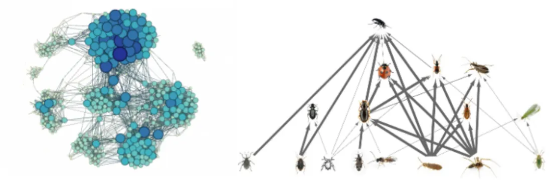
The field of complex networks aims at studying non-trivial interactions between entities by mean of a mathematical object called graph. A graph is a set of elements, called nodes, and a set of links, called edges, linking together a subset of nodes by pairs. This representation of information can be applied in a wide range of domains, going from transportation with for example the complex network of airline routes (where the nodes represent the airports and the edges the direct flight routes between two airports) to sociology (friendship, professional relationship), biology (proteins interactions, epidemic spreading) and many more.

Illustration 1 Example of a Facebook friendship network (left) adapted from http://datasciencepost.com/en/visualize-your-facebook-network-with-gephi/, where each node represents a Facebook user, and each link a friendship connection; a food web (left) from (Bohan et al. 2017).

Complex networks have also found applications in neuroscience. Indeed, the brain exhibits patterns in the functional interactions of its parts or in their structure that are unique to individuals and that can be modelized using graph theory. Those models constitute what is called the brain connectivity. Brain connectivity can be of different type; one can have: (i) structural

connectivity (SC); where links represent axons or neuronal fiber tracts or (ii) functional connectivity (FC) where links represent statistical dependencies between parts of the nervous systems. Those parts can be of different sizes leading to networks describing the brain connectivity at different scales. Depending on the spatial resolution of the physical measurements it is based

(19)

on, the “part” can be a single neuron (in that case the brain connectivity network is called a

connectome1_{), an ensemble of neurons, or brain regions.}

A neurodegenerative disease, such as Parkinson’s, Alzheimer’s, or Huntington’s disease, causes the neurons, building blocks of the nervous system, to progressively degenerate or die. Neurons lose their structure and/or functions. That is why brain connectivity analysis is particularly suited to study this kind of diseases, their impact by comparing to healthy brains, or even their progression through time. It gives an understanding of the brain structure or function as a whole, and allows to quantify the effects of the disease on different aspects. In particular, this manuscript will focus on Alzheimer’s disease’s impact on brain connectivity. The knowledges about this disease are really poor; clinically it is characterized (in order of appearance) by short-term memory disorders, loss of language and motor skills, disorientation, confusion and long-short-term memory disorders; neuropathologically, by the accumulation of tau protein extracellular neurofibrillary tangles and of intracellular amyloid-β (Aβ) protein plaques. This is what causes neuronal loss and synaptic disruptions in specific cortical areas; and what made it being described as a disconnection syndrome (Buckner et al. 2005).

In the era of big data, more and more brain images, brain signals, cognitive tests scores, demographic or even physiological data can be acquired from a single patient in a reasonable amount of time. Understanding each one of this large quantity of data is a problem in itself but understanding them all together is another story. In the field of brain connectivity, this can be translated to the use of multimodal, longitudinal, or high-resolution data.

This thesis report will expose how multilayer complex networks framework applied to brain connectivity could help understanding Alzheimer’s disease’s impact and progression. I will try to provide the reader with the right amount of information, references and links to work with multimodal brain connectivity; from raw brain data to abstract graph models.

In the first chapter, I will go through the basics of brain connectivity, presenting the widely used brain imaging modalities and their associated (pre-)processing steps necessary to access to a functional or structural connectivity estimate. I will then, in a second chapter, present a few formalisms from graph theory that have been applied to model brain connectivity networks. How

1_{At the time of writing, only one connectome has been fully described and is the one of a 2mm worm called Caenorhabditis}

(20)

Introduction 19 we manipulate them, what we can measure on them, and how these measures allowed us to learn about the brain and the impact that Alzheimer’s disease has on it. The third chapter will be dedicated to the multilayer topology and its application to brain connectivity; a short review of the literature will help the reader to identify the context in which the studies that constitute the three following chapters were conducted. Chapter 4 will illustrate a successful application of a specific type of multilayer topology called multiplex on a magnetoencephalography-based study of Alzheimer’s disease. Chapter 5 introduces a novel generalization of the concept of core-periphery structure in multiplex networks. And finally, chapter 6 apply this newly defined core-periphery model to the first three-modalities multiplex networks and gives new insights on the impact of Alzheimer’s disease on most important brain regions.

(21)

(22)

CHAPTER 1

Structural and

functional

brain

connectivity

I

Neuroimaging data

(23)

Magnetic Resonance Imaging, abbreviated as MRI, is a medical imaging technique based on a physical phenomenon called nuclear magnetic resonance (NMR). By the mean of strong magnetic fields and radio waves pulses that excite atoms (mostly hydrogen) present in biological organisms, it is possible to measure some of their NMR properties and deduce the nature of the tissue they are in. The obtained signals can be localized by small unitary volumes (in the order of 1mm3_{) called a}_voxel

(Illustration 2).

Repeating this operation for adjacent voxels allows to obtain a set of signals covering the entire desired volume. Finally, depending on the physical measure extracted from those signals and on the radio waves trains used to generate them, and on a lot of other physical conditions, a large variety of contrasts can emerge between the voxels allowing the creation of different 3D volumes (or scan) that are usually visualized by slices, i.e. 2D images.

Among the most used MRI techniques, one can present the following ones:

o T1- and T2-based MRI: based on their respective relaxation time (denoted !" and !#) needed by an excited atom to retrieve a stable state. These contrasts are the core of

almost every clinical MRI protocol (Symms et al. 2004).

o fMRI: functional MRI, based on the blood-oxygen-level dependent contrast (BOLD).

o DWI: diffusion weighted imaging, based on the measure of the Brownian motion (random motion of water molecules).

i

T1- and T2-weighted MRI

As mentioned above, these two contrasts are the basis of all MRI-based studies. T1 is mostly used to study normal anatomy while T2 is more appropriate to identify lesions.

Illustration 2 Artistic representation of the voxels present in a human brain 3D scan.

(24)

Structural and functional brain connectivity 23

They are fast, thus reducing the risk of movement by the patient during the scan which makes them the least susceptible to image artifacts. And with a high spatial resolution, they allow to precisely segment the brain in to white matter (WM), gray matter (GM), and cerebrospinal fluid (CSF) (Illustration 4 ). A wide variety of automated segmentation techniques now exist (Liew and Yan 2006; de Boer et al. 2010) to deal with images data that are getting larger and larger2

and for which it would take days for a trained anatomist to segment manually

T1 images are also used to measure volumes of different brain parts, such as the hippocampus, or the global atrophy of the cortex by evaluating its thickness (Illustration 4 ). They give the reference 3D volume on which any further scans can be registered to.

ii

fMRI

Functional MRI, as its name implies, gives information about the brain activity but is not a direct measure of neural activation. It is based on the BOLD contrast, first described in (Ogawa et al. 1990), that follows the blood oxygenation which itself reflects the demands in glucose, only source of energy of normal brain cells.

This contrast is limited in spatial - due to long range magnetic susceptibility - and temporal resolution due to the slow speed of the hemodynamic response. Also, the signal changes related

2_{7T T1-weighted ultra-high resolution images can now weight more than 1 TB (Lüsebrink et al. 2017)}

Illustration 4 Segmentation of the cortex. Gray/White matter (yellow) and pial (red) surfaces (Fischl and Dale 2000).

Illustration 3 Example of a brain tumor visualization on a T1- and T2-weighted MRI scans. Adapted from

(25)

to cerebral activation are close to the noise level which led to numerous controversial results in the literature, especially when they are not corrected for multiple testing (Bennett, Wolford, and Miller 2009).

iii DWI

Diffusion represent the random movements of molecules (Brownian motion). In DWI, one study the diffusion of water molecules, largely present in the brain cells or in the CSF, by measuring its magnitude in a given direction with the appropriate MR sequences.

Figure 1.1 Graphical display of water molecules moving at different rates through the gray matter and cerebrospinal fluid (CSF). The effective distance that water molecules travel in gray matter is smaller than in CSF (represented by the magnitude of the red arrow). The difference in travelled diffusion distance versus time is displayed in the lower graph. The faster the molecules move, the more distance is travelled, the more signal loss will occur if diffusion gradients are applied. Consequently, the signal loss in the CSF is higher (hypointense) compared with the signal loss in the gray matter (hyperintense relative to the CSF). Extracted from (Huisman 2010).

Diffusion in brain tissues can be isotropic, such as in CSF or any other liquid in which the water can diffuse equally easily in each direction, or it can be anisotropic, such as in white matter that has an internal fibrous structure favoring diffusion of water in the direction of the main fibers (Huisman 2010). Therefore, the DWI contrast is dependent on the direction of the applied gradient.

(26)

Structural and functional brain connectivity 25 By repeating the acquisition of DWI volumes for different gradient directions (three can be enough), one can build the diffusion profile (which is often summarized in a tensor and represented as an ellipsoid, see Illustration 5) at each voxel and thus deduce the main direction of propagation of the water molecules, it’s called

diffusion tensor imaging (DTI) (Peter J. Basser et al. 2000). From these, one can calculate various maps, such as:

o the mean diffusivity (MD), sometimes called apparent

diffusion coefficient (ADC), it reflects the rotationally invariant magnitude of water diffusion within brain tissue (Clark et al. 2011); o the fractional anisotropy (FA), a scalar between 0 and 1 which measures how

asymmetric the diffusion inside a voxel is;

o the principal diffusion direction, usually referred to as colored FA (cFA) where the voxel hues are reflecting the main tensor orientation (usually with red indicating transverse,

green indicating anterior–posterior, blue indicating superior–inferior; “RGB for xyz”) and voxel brightness weighted by FA.

B

EEG/MEG

Electroencephalography (EEG) and

magnetoencephalography (MEG) are monitoring methods used to respectively record brain electrical fields and brain magnetic fields. The EEG and MEG are very close methodologies, since the main sources of both kinds of signals are essentially the same, i.e., ionic currents generated by biochemical processes at the cellular level (Lopes da Silva 2013). While EEG consist in a set of electrodes to be placed in contact with the surface of the head and connected to a relatively small device, MEG is a large machine under which the subject has to place his head, inside a magnetically shielded room.

For an electric or magnetic signal to be recordable at a distance, a large enough assembly of neurons should activate in a coordinated way and be spatially organized. That is the case of a family of neurons called pyramidal cells. In order for electromagnetic fields to reach distant sensors, various tissues must be passed. The different layers, such as the

Illustration 5 Visualization of DTI data using ellipsoids.

Illustration 6 high resolution 256 electrodes EEG setup from

http://dreamsessions.org/101artwork s.html.

(27)

cerebrospinal fluid, skull, and skin, especially affect electric fields due to their different electrical conductivities but have less impact on the magnetic fields that are not distorted by scalp or skull for instance. However, the magnetic fields diminish as 1/&'_{with the distance of & (Singh 2014).} EEG and MEG are subject to the problem of source localization. In many applications it is important to know from where the electromagnetic signal came from. The estimation of the sources from the scalp fields is called inverse problem. It is ill-posed and consequently, has an

infinite number of solutions that need to be restrained by making assumptions on the nature of the sources. A large number of methods exist whose details go beyond the subject of this manuscript; for reviews on EEG/MEG source imaging (MSI) techniques, see (Michel et al. 2004; Grech et al. 2008; Becker et al. 2015).

Both modalities have their advantages and drawbacks. MEG is more sensitive in detecting currents that are tangential to the scalp whereas EEG is sensitive for both tangential and radial currents. This makes MEG detecting primarily the “fissural” cortex activities (i.e. activities present in the sulci). MEG is said to have a better spatial resolution with 4cm2 on scalp and 3-4mm when its signals are source-localized (Singh 2014). But it is also a lot more expensive than EEG, and has logistic constraints that could make difficult for research or clinical facilities to acquire it and/or run specific protocols.

Although the human brain produces activity in a wide range of frequencies (0.5 to 500 Hz), the most clinically relevant activities lie below 70 Hz (normal physiological or spontaneous waves) and the frequency bands are alpha (8 to 13 Hz), beta (13 to 30 Hz), theta (4 to 8 Hz), and delta (1 to 4 Hz). (Velmurugan, Sinha, and Satishchandra 2014)

II Structural and functional connectivity

A Concept and motivation

It has been shown that the human cerebral cortex is composed with distributed neural assemblies, densely connected and interconnected to form a large-scale cortical circuit or “web-like” structure (Varela et al. 2001; Boccaletti et al. 2006; Schnitzler and Gross 2005; Carter, Shulman, and Corbetta 2012). In that context, a connection is often said to be structural or functional.

(28)

Structural and functional brain connectivity 27 The structural (or anatomical) connectivity (SC) corresponds to the physical connection between different brain sites. At a microscopic scale, those connections can correspond to synapses whereas at a more macroscopic level, when we study neural ensembles or cortex parcels, we observe white matter fiber pathways or tracts that are estimated using tractography algorithm based on DTI data (see section “Structural connectivity estimators” for more details). While this set of connections is quite stable at shorter time scales (seconds to minutes), it can be altered at longer time scales (hours and more) by a phenomenon called plasticity consisting in the strengthening/weakening of synapses or the remapping of cognitive functions to different cortical locations. These changes may be due to training (environmental stimuli), thoughts, emotions or injury.

The functional connectivity is a statistical concept defining how dependent spatially distant neurophysiological activities are. Due to the wide variety of neural activity recording methods and to the fact that, for most of these methods, activities recorded at one site may be influenced by its surrounding neighborhood (i.e. because of volume conduction), no unified definition of functional connectivity exist. For voxel-based modalities, such as fMRI or PET, the studied brain “sites” can be a single voxel or voxels aggregates, whereas sensor-based modalities, such as EEG or MEG, offer a choice between working directly with sensors or with reconstructed sources (De Vico Fallani et al. 2014).

In the framework of complex networks and to understand the systemic impact of wide spread neurodegenerative diseases such as AD, we build an interconnected representation of the brain based on those two concepts, a whole brain connectivity network or more concisely a brain network (Simpson and Laurienti 2016). In whole brain networks the connectivity is computed between all possible pairs of brain voxels, cortex parcels or white matter volumes that act as the nodes of the network. There are usually two families of scales at which functional or structural connectivity brain networks are computed: voxel/vertex-level or region-level. In the former, signals and images are kept in their thinner spatial resolution possible - the voxel in the case of MRI-based data, and the vertex or the sensor in EEG/MEG data. At this scale, the signals may be noisy or suffer from reconstruction algorithms limitations. Moreover, dealing with millions of time series might be computationally challenging. In the latter family of scales, time series or white matter tracts are aggregated in small brain regions following a brain parcellation.

(29)

B

Brain parcellation

The choice of a parcellation is an important one, it will determine the number of nodes that the brain networks will be composed with, and thus the granularity of the brain connectivity profile. Grouping together cortex sub-parcels with opposite behaviors (functional or structural) into one single entity might generate, by average, a cancelation of its contribution in the whole network. Brain parcellation is a real topic of research, as can attest the number of papers gathered in the past year by a single review by Craddock, Bellec, and Jbabdi (2018). This special issue reviews all the latest methods related to this domain going from cytoarchitecture-based manual parcellation to fully automated whole brain segmentation using deep learning. The importance of this aspect of brain connectivity is such that the well-known MICCAI international conference organized a challenge on this topic in 2013: MRBrainS (http://mrbrains13.isi.uu.nl/, Mendrik et al. 2015)

A large panel of brain parcellation methods exist, but the most commonly used in the field on brain networks can be divided in two categories; anatomy- or connectivity-based parcellation.

i

Anatomy-based parcellation

Traditionally, anatomical brain atlases or templates are used to define regions of interest

(ROIs), i.e. the nodes of the whole brain network. These atlases are derived from anatomical landmarks, cortex curvatures, or cytoarchitectonic3_{information. Then, the standard pipeline is}

the following: one or more subjects’ anatomical images (usually T1) are manually parcellated, and registered onto the average brain in order to obtain a template brain. All new subject is then registered on this template which propagates its region labels onto the subject’s brain in order to parcellate it (de Reus and van den Heuvel 2013).

3_{Architecture of neural cells}

(30)

Illustration 7 Example of the Desikan-Killiany anatomical parcellation. 34 ROIs are delineated on each hemisphere based, mainly, on local curvature.

For example with the Desikan-Killiany atlas (Desikan et al. 2006) the procedure was to manually parcellate the cortical surface of 40 brains coming from various profiles (different sex, age, condition) based on heterogeneous information including: standard conventions, previous atlas definitions, and local curvature. They generated an atlas by mean of a registration - i.e. the cortical folding patterns alignment - and probabilistic assignment of a label to each vertex of the cortical surface. 34 parcels on each hemisphere. A similar process was also used for the Destrieux atlas (Christophe Destrieux et al. 2010) which is based on the work of (Duvernoy 1999) and ended up being composed with 148 ROIs. Both of these parcellation can be automatically

generated using the largely distributed FreeSurfer software

(https://surfer.nmr.mgh.harvard.edu/) making them ones of the most used anatomical parcellations.

(31)

The Automated Anatomical Labeling (AAL) (Tzourio-Mazoyer et al. 2002) is another widely used brain parcellation also based on cortical curvature and standard nomenclature but it has the following advantages: (i) it is freely available inside the SPM software (Litvak et al. 2011); (ii)

it provides a volumetric parcellation (and not only a parcellation of the cortical surface) adapted for fMRI-based functional connectivity; (iii) it has been defined directly in the MNI space4_from

the high resolution Colin275_{brain; and (iv) the number of ROIs (or AVOI, as described in the}

paper) is particularly suited for a brain connectivity analysis at reasonable scale.

Illustration 8 Regions of interest of the AAL atlas (Tzourio-Mazoyer et al. 2002), drawn on axial 1-mm-thick T1 MNI single-subject slices (only one slice every 4 mm is reproduced). Values on the lower right of each slice indicate the stereotaxic z coordinate in millimeters (from ) = 75 to ) = 19 mm).

4_{The MNI space consists in the average of 305 (then 152) T1 brain scans linearly transformed to the Talairach stereotaxic} template.

5_{T1 brain template computed as the average of the 27 scans of a single young man. After a non-linear registration to the} MNI305 space, this template has been adopted by many standard software e.g., AFNI (Cox 1996); Brainstorm (Tadel et al. 2011); SPM (Litvak et al. 2011); Fieldtrip (Oostenveld et al. 2011).

(32)

Illustration 9 Regions of interest of the AAL atlas (Tzourio-Mazoyer et al. 2002), drawn on axial 1-mm-thick T1 MNI single-subject slices (only one slice every 4 mm is reproduced). Values on the lower right of each slice indicate the stereotaxic z coordinate in millimeters (from ) = 13 to ) = −43mm).

This parcellation method have some limitations. First, inter-individual anatomical variability (Zilles et al. 1997; Destrieux et al. 1998) which remains from 9 to 18 mm, depending on the brain regions considered (Thompson et al. 1996). Second, the heterogeneity of structural and/or functional connectivity inside each macroscopic brain parcels. For example, the works of Margulies et al. (2007) and Beckmann, Johansen-Berg, and Rushworth (2009) showed respectively that structural and functional connectivity in the anterior cingulate (AAC) was highly heterogenous thought it was typically represented as a single ROI (in AAL for instance, Arslan et al. 2018).

ii

Connectivity-based parcellation

The common concept between most of the connectivity-based parcellation (CBP) algorithms is to cluster vertices or voxels of the brain images/signals based on a local similarity measure such as Pearson’s correlation, Euclidian distance, etc.; or on a global metrics such as Newman’s modularity (see Chapter 2 for more details), using various unsupervised clustering algorithm such

(33)

as k-means, hierarchical clustering (Ward Jr. 1963) or spectral clustering. A spatial constraint is usually added such that only neighboring clusters or voxels/vertices can merge into one single cluster. Most CBP are single-subject’s parcellations; their scan-to-scan reproducibility, thus, cannot be assured. But being directly obtained from the underlying data, they can provide much more coherent parcels for subsequent connectivity analysis.

Illustration 10 Typical example of connectivity-based parcellation procedure from Blumensath et al. (2013). After preprocessing, clustering proceeds in four steps. In step (1) a slightly smoothed stability map is computed (black: more stable, red: less stable). Local optima are identified in step (2). The locations of these optima will be the seed regions used in the next step. In step (3) the seeds are grown into disjoint clusters, giving the finest clustering. Finally, in step (4), a spatially constrained hierarchical clustering method builds a cluster tree, giving not only a single parcellation, but an entire spectrum of parcellations at different resolutions (only one of these is shown here).

There is a growing list of exhaustive reviews specifically treating the subject of CBP: Eickhoff et al. (2015), Thirion et al. (2014), and de Reus and van den Heuvel (2013).

“Importantly, no single package permitting CBP is, to the best of our knowledge, openly distributed at the moment. Rather, it seems that different research groups perform CBP analyses based on their own script library, in-house databases, and laboratory setups. However, sharing of code implementations and international collaboration on its successive improvement will hopefully contribute towards a widely accepted software infrastructure (cf. Pradal, Varoquaux, and Langtangen 2012).”

(34)

Structural and functional brain connectivity 33 CBP algorithms have been evaluated again this year by Arslan et al. (2018) which associated to their paper a website (https://biomedia.doc.ic.ac.uk/brain-parcellation-survey/) that lists some links to some of the source codes used to generate the parcellations and a GitHub repository containing all the scripts used to evaluate the 24 parcellations as depicted below.

C

Connectivity estimators

Once the nodes of the brain network are chosen, depending on the modalities available, you can define the links between them using a connectivity estimator.

i Structural connectivity estimators

Structural connectivity almost exclusively refers to a quantification of the white matter fiber tracts density or quality computed using tractography algorithms on DWI images. A tractography algorithm can be divided in two steps: (i) the local modeling, which defines at each voxel the distribution of directions of propagation; and (ii) the fiber tracking that uses this local information to build 3D trajectories called streamlines or fiber tracts (Yo et al. 2009; Khalsa et al. 2014).

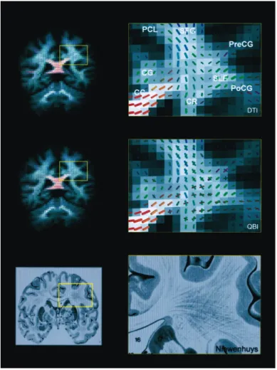
Two types of local models exist: the one, most common, describing a single main fiber orientation of whiter matter inside each voxel, known as the diffusion tensor model (DT, P J Basser, Mattiello, and LeBihan 1994); and those capturing multiple fiber orientations such as the multiple tensor model (Tuch et al. 2002), 2-ball imaging (QBI, Tuch et al. 2003), diffusion spectrum imaging (DSI, Cohen Veterans Bioscience n.d.), [constrained] spherical deconvolution

(Tournier et al. 2004; Tournier, Calamante, and Connelly 2007), etc. (review by Alexander 2005; Lazar 2010). The former type of methods has been proven limited since it cannot capture crossing/kissing/fanning/branching fibers inside a single voxel (Seunarine and Alexander 2014; Jones 2010).

(35)

Illustration 11 Comparison of DTI, QBI, and Nieuwenhuys Atlas.(Tuch et al. 2003)

Some of those advanced methods may require specific DWI sequences with, for example, a set of different 3-values6_{, high 3-values (3 > 3000s/mm}2_{), or many gradient encoding directions} (8enc> 60) such as models based on high angular resolution diffusion-weighted imaging (HARDI, Tuch et al. 2002). These setups may lengthen the time necessary for a scan, thus, making them not suited in clinical environments where young, diseased or old patients cannot support long periods inside an MRI scanner.

After the local modeling, the fiber tracking algorithm allows to estimate fiber tracts. The algorithms usually work as follow: a seed voxel is randomly chosen within a subset of possible voxels to start from, then a streamline starts to grow by making steps towards either (i) the most probable direction as dictated by the local model of the voxel in question - this is called

deterministic tractography - or towards (ii) a direction sampled from the local fiber orientation

6_{The 3-value is a factor that reflects the strength and timing of the gradients used to generate diffusion-weighted images.} (“B-Value Diffusion” n.d.)

(36)

distribution (FOD) - this is probabilistic tractography. The most common deterministic tractography algorithms are FACT for Fiber Assigned by Continuous Tracking (Mori et al. 1999) or the streamline tracking algorithm (Peter J. Basser et al. 2000).

In practice

In order to compare all the variety of different preprocessing pipelines and tractography algorithm, a first initiave called FiberCup (Fillard et al. 2011) tried to define a common framework under the form of a challenge. More recently, Maier-Hein et al. (2017) reviewed 96 methods of tractography and associated a standalone tool to evaluate new submission (http://tractometer.org/).

Another interesting initiative is the gathering of HARDI-based methods in a MATLAB®_toolbox

(“NeuroImageN - High Angular Resolution Diffusion Imaging (HARDI) Tools” n.d.).

Once the set of tracts (or tractogram) is generated, different connectivity measures allow to quantify the strength of the connection between two ROIs. The most common one is known as number of streamlines (NOS) and simply counts the number of generated fiber tracts connecting the two sets of voxels/vertices, i.e. starting in ROI = to finish in ROI >. Some other estimators use the length of the fiber tracts as a factor of the weight (Hagmann et al. 2008), and/or normalize it by the size (area, number of vertices/voxels) of the connecting ROIs. One can also weight the connection based on its probability (for probabilistic tractography-based methods), or on the fractional anisotropy (FA) of the voxels it’s crossing.

ii

Functional connectivity estimators

The standard approach in functional connectivity is to estimate a statistical dependency between time series averaged inside each previously define ROI. Functional connectivity estimators can be

linear/nonlinear, bivariate/multivariate, in the time/frequency domain or even based on

information theory.

The simplest, linear, is the cross-correlation, especially and widely used in fMRI-based connectivity analyses (introduced by Cao and Worsley (1999) discussed by Zalesky, Fornito, and Bullmore (2012) and Hlinkaa et al. (2011)). Another similar measure is the (sometimes called magnitude-squared-, spectral-, or phase-) coherence equivalent to the cross-correlation, but in

(37)

the frequency domain. It captures linear time-invariant relationship between two time series by resulting a coefficient between 0 and 1; 0 meaning no linear relationship, and 1 meaning that one time series can perfectly predict the other in a linear way, independently of the phase difference as long as it doesn’t change through time (i.e. time-invariant) (Sun, Miller, and D’Esposito 2004). Coherence is function of the frequency and is usually averaged by frequency bands that have a neurophysiological meaning; making it the preferred connectivity measure for wide frequency range brain recordings (typically EEG and MEG). The phase lag index (PLI, by Stam, Nolte, and Daffertshofer (2007)) that works as a phase synchronization quantifier or the wavelet correlation and its multiresolution nature (Bullmore et al. 2004; Achard et al. 2006) are also adapted to time series of neural activities.

Illustration 12 Illustration of coherence as a measure of the linear time-invariant relationship between two time series. In this simulation, the same model of neural activity is linearly convolved with two different models of the hemodynamic response function. The correlation coefficient of the resulting time series is 0.52, which is low compared to the coherence in the bandwidth

of the hemodynamic response function (HRF). Within the bandwidth of the model HRF, coherence is near 1, and above the HRF bandwidth, coherence is near 0. (Sun, Miller, and D’Esposito 2004)

Granger causality is very well appreciated for its directed aspect. Indeed, the granger causality evaluates differently the connection from node = to node >, from the one from > to =. It is said that = causes > if the past information contained in the signal of = helps in predicting the signal of >. Many other dependency estimators exist such as the directed transfer function (DTF, by Kaminski and Blinowska (1991), the phase locking value (PLV, by Lachaux et al. (1999)), the partial directed coherence (PDC, by Baccalá and Sameshima (2001)), the synchronization likelihood (SL, by C. J. Stam and van Dijk (2002)), or the imaginary part of coherency (Nolte et al. 2004). And novel methods based on deep learning are also appearing (Y. Wang et al. 2018). Colclough et al. (2016), Sakkalis (2011) and Jalili (2016) reviewed some of the connectivity estimators and discussed the binarization methods.

(38)

CHAPTER 2

Complex brain

networks

I

Brain network as a graph

A set of connectivity coefficients for each pair of ROIs can be stored in a 8 × 8 matrix, with 8 the number of ROIs, called an adjacency matrix @ = ABCDE, ∀=, > ∈ 1. . 8, where BCD is the connectivity coefficient (or weight of connection) between ROI = and ROI >. It can be represented as a fully connected graph of 8 nodes, and 8 × (8 − 1) directed (or L×(LM")_# undirected) edges weighted by their corresponding coefficient in @. Basic operations on @ are (i) the thresholding that allows to remove weak links that may be spurious and due to noise in brain signals and images; (ii) binarization that can be useful when the strength of a link does not really make sense (such as in structural connectivity analysis where you could simply be interested if there is a connection or not) nor directly reflect the real physiological phenomenon (iii) symmetrization, less usual, permits the conversion of directed to undirected links, when the direction of the connection is not of interest after a wrongly chosen connectivity estimator.

Thresholding generates information loss, but is often adopted to remove spurious links, reduces the false positives rate, and simplify the resulting network topology. It may be absolute, or

proportional; it is, in many cases, arbitrarily chosen. While some studies analyze networks across broad range of thresholds, a recent study have attempted to estimate a priori an optimal threshold

(39)

value based on topological hypotheses (De Vico Fallani, Latora, and Chavez 2017), or other more standard methods filter networks based on the statistical significance of each link (Gourévitch, Bouquin-Jeannès, and Faucon 2006; Toppi et al. 2012; Craddock et al. 2013) which again depends on an arbitrarily chosen “significance” threshold. There exists other network filtering techniques that try to somehow optimize the topology of the network, such as by extracting the minimum spanning tree (MST) or minimum connected component (MCC), defined respectively as the subgraph minimizing the summation of link weights without forming any loops and the subgraph removing the weakest edges as soon as all the nodes are not disconnected from the main component (Vijayalakshmi et al. 2015; Jalili 2016).

(40)

Complex brain networks 39

Illustration 13 Visual representations of brain networks’ adjacency matrices and their associated graph after standard connectivity estimation and manipulation. Each rows and columns representing nodes and matrix entries representing links weighted by a connectivity estimator. Most of the connectivity estimators allow to start with a fully-connected and weighted network (top row) that are often reduced to sparse binary undirected form (bottom row) through thresholding, binarizing, and symmetrizing (Rubinov and Sporns 2010).

Binarizing and symmetrizing also generate great loss of information but also facilitate a lot the analysis, with in practice, a decreased computation time and power necessary for every operation (including visualization), simple graph metrics and more easily defined null-models for statistical comparisons (see below).

(41)

II Graph analysis tools

A Graph metrics

The brain networks topology can be quantified by metrics coming from graph theory. These are often segmented in function of the scale of the entity they are describing, that might be a single node, the local scale; a group of nodes (or modules), the mesoscale; or the whole network, the

global scale.

Starting with local measures, the most standard is the node degree dO which is the number of nodes to which a given node is connected and can mathematically written as follow:

PC= Q RCD DSC

,

where RCD are the entries of the binarized adjacency matrix (zeros or ones). The degree reflects the centrality, i.e. the importance of a node in comparison with all the other nodes of the network. A lot of network metrics are derived from this first one, including the network density ρ or normalized average degree:

U = 1 8 − 1× PV = 1 8 − 1× 1 8Q PC C ,

With PV the average node degree, U is comprised between 0 for disconnected networks and 1 for fully-connected networks (normalized by 8 − 1, the maximum degree of a node). Note that global measures are usually averaged versions of local measures across the whole set of nodes.

i

Functional integration metrics

such as for the global efficiency E, which is inversely proportional to the average shortest path length: X = 1 8Q XC C = 1 8Q 1 8 − 1× 1 ∑DSCZCD, C

(42)

Complex brain networks 41 With ZCD the shortest path length between node = and node > and XC the efficiency of node = (local, but different from the “local efficiency” of node =, see below). This measures how globally efficient a network is in the sense of connecting distant nodes together. Global efficiency is related to another measure based on shortest paths called characteristic path length (Watts and Strogatz 1998): [ = 1 8Q [C C = 1 8Q ∑DSCZCD 8 − 1 C ,

Where [C is the average distance between node = and all other nodes (local).

These two latter measures reflect the functional integration of the concerned network. Functional integration is the brain’s ability to combine (integrate) information from distributed (long distance) brain regions. Here the distance definition depends on the type of brain network in question; it could be structural, functional or even metric if, for instance, your distance ZCD is defined as the physical distance separating two brain region’s centroids based on a structural connectivity-based network topology. Though, the relationship between X, [ and functional integration should be taken with care as highlighted by Achard and Bullmore (2007) and Estrada and Hatano (2008) since they do not take into account the redundancy of paths (and their length, longer than or equal to the shortest ones) connecting pairs of nodes.

Other local measures make use of the shortest paths in order to characterize the centrality of a nodes or edges, they are called node betweenness centrality NBCO and edge betweenness centrality EBCO_ respectively and represent the number of all-to-all shortest paths making use of a given node or edge respectively. They can be defined as follow:

8`aC= Q Γcd(=) Γcd cSCSd , and, X`aCD= Q ΓcdefCDg Γcd cSd ,

where Γcd is the number of shortest paths between node h and i, Γcd(=) the number of these paths making use the node =, and Γjk(fCD) those making use of the edge between node = and >.

(43)

ii

Functional segregation metrics

We say that the brain is functionally segregated if groups of brain regions are densely

intraconnected but sparsely interconnected. Those groups of nodes are called modules, clusters, rich-club, core or community structure and can be quantified using the following metrics. First, the clustering coefficient C, which is the fraction of the node’s neighbors that are directly connected to each other (Watts and Strogatz 1998); or put differently, the number of triangles a given node belongs to over the total number of triangles it could belong to.

a = 1 8Q aC C =1 8Q 2!C PC(PC− 1) C ,

Where !C is the number of triangles around node = and could be written as !C = "

#∑ RD,l CDRClRDl, and aC is the (local) clustering coefficient of node =. A variation of the clustering coefficient that stays in a similar spirit is the local efficiency Eloc (different from the local version of the efficiency EO, that measures how close a node is from any other nodes of the network). This one

characterizes, like the clustering coefficient, and unlike the global efficiency, only the neighborhood of a given node i but instead of looking at direct connections between them, it puts emphasis on the length of the shortest path linking them.

Xloc= 1 8Q Xloc,C C = 1 8Q ∑D,p∈qrZDpM" PC(PC− 1) C ,

Where sC is the subgraph containing all the neighbors of =, but not =. For an extensive comparison between a, X, Xloc, and [, see the work of Latora and Marchiori (2003).

The segregation in a network can also be characterized globally through the concepts of community structure and modularity. The range of algorithms used to divide a network into partitions of densely connected nodes that are sparsely connected together is vast and complex but a majority of them are based on the modularity index Q (Newman 2004, 2006) defined as follow: t = Q u2vv− wQ 2vx y xz" { # | y vz" ,

(44)

Complex brain networks 43 With } the number of modules and 2vx the proportion of all links connecting nodes in module ~ with those in module . Finally, the participation coefficient PC, based on a previously computed partition of modules, evaluates how evenly distributed the connections of a given node are across module. It is defined as follow:

ÄaC= 1 − Q Å PC(~) PC Ç # y vz" ,

With PC(~) the number of connections the node = with nodes belonging to module ~.

iii

Other metrics

All the metrics presented above have been described in the context of a binary adjacency matrix, i.e. an undirected unweighted network, but adaptations exist for both directed and weighted networks. Also, a lot of other graph metrics exist, but I presented here the most useful ones for brain connectivity analysis, or at least, the most common.

In practice

Jalili (2016) reviewed a set of networks measures useful in brain connectivity analysis. And Rubinov and Sporns (2010) made an amazing work in summarizing a large number of metrics for which they provided source codes in their MATLAB®_{brain connectivity toolbox}

(https://sites.google.com/site/bctnet/) along with graph manipulation algorithms such as null models generation or thresholding. For Python users, the networkx library is now a standard

and efficiently implemented a large number of metrics (https://networkx.github.io/documentation/networkx-1.10/reference/algorithms.html).

B

Null-hypothesis networks

Since most of the network measures indirectly depends on basic topological attributes such as the number of nodes, the number of edges or the degree distribution which themselves depend on the parcellation and/or connectivity estimator; comparing two networks extracted from different subjects, or even different machines become difficult. Therefore, significance of network indices must be computed against null-hypothesis networks, i.e. random networks that share the

(45)

topological attributes of the original one but are not supposed to expose any specific behavior that could be captured by the index in question.

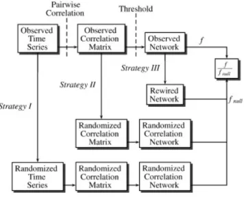
Figure 2.1 Strategies for generating null networks. Strategy I: time series randomization. Strategy II: correlation matrix randomization. Strategy III: topology randomization (e.g. random rewiring). É denotes the network measure calculated for the observed network, while Énull denotes the same network measure averaged over the ensemble of null networks. Adapted from Zalesky,

Fornito, and Bullmore (2012).

Different strategies are presented in Figure 2.1, at different steps of the brain connectivity network creation pipeline. Each of them has their advantages and pitfalls, but a common approach is to randomly rewire (strategy III) the final networks while preserving the degree distribution. While this method’s algorithm is quite simple for binary networks, it might become theoretically and computationally complex for weighted and/or directed networks. The only - probably obvious - rule is to choose a null model for which the original network topology does not have any influence from the point of view of the metric of interest; or, on the contrary, a null-model that greatly impact a metric. For example, time series randomization would generate networks with different densities if analyzed using a fixed threshold value; then studying a metric that depends on shortest path lengths would not make much sense since sparser (resp. denser) networks would have much more probability to have longer (resp. shorter) path lengths.

III Known characteristics of brain networks

(46)

Complex brain networks 45 The concept of small-world comes from a social experiment known as the Milgram paradox

(Travers and Milgram 1969) stating that two people, from anywhere in the world, are separated by a small number of intermediates. Put differently, in the world’s social network, where nodes are people and links are relationships, the characteristic path length is small (around six, according to experiments that followed Milgram’s). This phenomenon was studied through the lens of complex networks by Watts and Strogatz (1998), by mean of randomization of a lattice network, and latter quantified thanks to a small-worldness index S (Humphries, Gurney, and Prescott 2006) defined as follow:

Ö =a/arand [/[rand,

Where a and [ are the clustering coefficient and the characteristic path length as defined in section “Graph metrics”. arand and [rand are the same measures for equivalent random networks with an identical number of nodes 8 and identical density U. A network is considered to have a high small-worldness when its characteristic path length is significantly shorter than for equivalent random networks and have, in the same time, a higher clustering coefficient than by random. Thus, it should be a balance between integration and segregation to be robust to single-node failures while keeping a cost-efficient propagation of information thanks to smartly distributed shortcuts (Bassett et al. 2006).

Human (and other mammalian) structural brain networks extracted from DWI have high-degree nodes, or hubs, and modular structure giving it small-world networks properties (Bullmore and Sporns 2009; Hagmann et al. 2007; Heuvel and Sporns 2011). This result has also been demonstrated in functional brain networks.

Bassett and Bullmore (2017) review the latest advances on this concept of small-world network and put emphasis on its generalization to weighted networks that carry much more information than the old simple but still popular unweighted/binary network model of the brain. In particular, it draws attention on weak connections that may play an important role in brain connectivity of both healthy and diseased.

(47)

The default mode network (DMN) was observed by Shulman et al. (1997) who noticed a set of brain regions whose activity was reduced when performing non-self-referential, goal-directed tasks as compared to a control state of quiet rest or simple visual fixation. It was originally measured using positron emission tomography (PET) imaging7_{(Raichle et al. 2001), where}

the “activity” was defined as an increase of the oxygen extraction fraction (OEF), a ratio of

oxygen consumed to oxygen delivered. But this effect can be detected in standard fMRI scans, even though the relationship between blood-flow and oxygen consumption may not be completely evident (Raichle and Mintun 2006).

In AD, relationships between amyloid-β (Aβ) deposition and the DMN have been observed (Buckner et al. 2005; Vlassenko et al. 2010; Mormino et al. 2011) as shown in Figure 2.2. Buckner, Andrews-Hanna, and Schacter (2008) mention the possibility that activity in the default network augments a metabolic cascade that is conducive to the development of Alzheimer's disease.

The brain can also expose other more or less identified sub-networks such as visual, sensorimotor, auditory, ventral and dorsal attention, and executive control (Raichle 2010; Betzel et al. 2014). A recent paper from Raichle (2015) himself retraces the history of the DMN and its impact on the literature.

7_{PET is a functional imaging technique used to visualize metabolic processes in the body. It measures gamma-rays emitted} by a position-emitting radioactive isotope usually embedded on an analogue of glucose molecule (called fludeoxyglucose) that serves as radiotracer. This allows to indirectly obtain 3D images of energy (i.e. glucose) consumption in the body by triangulating gamma-rays emission and evaluating the radiotracer concentration.

(48)

Complex brain networks 47

Figure 2.2 Convergence and hypothetical relationships across molecular, structural, and functional measures. This figure shows how default activity (DMN) pattern in young adults is highly similar to those of amyloid deposition in older adults with AD. Extracted from Buckner et al. (2005)

C

Structural rich-club

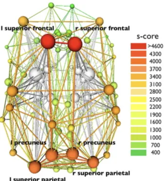
A few studies have tried to identify hub regions in structural brain networks. Hubs are central nodes sharing high degree, strength and/or betweenness centrality. Hagmann et al. (2008) mapped whole brain structural pathways (between 8 = 998 ROIs) of five participants using diffusion spectrum imaging (DSI) followed by a tractography and found evidence for the

existence of a structural core composed of posterior medial and parietal cortical regions that are densely interconnected and topologically central (see Figure 2.3). They emitted the hypothesis that those regions may play an important role in information integration and showed that the strengths of structural connections were highly predictive of the strengths of functional connections.

Figure 2.3 Average network core after the k-core decomposition of five subjects’ binary connection matrix. Adapted from Hagmann et al. (2008).

en fr

HAL Id: tel-01985286

https://tel.archives-ouvertes.fr/tel-01985286v2

Alzheimer’s Disease

Jérémy Guillon

To cite this version:

Multilayer Approach

to Brain Connectivity

in Alzheimer’s Disease

J

ÉRÉMY

G

UILLON

Sorbonne Université

Approche multi-niveaux de la

connectivité cérébrale dans la maladie

d’Alzheimer

Table of

contents

Table of contents ... 5

Remerciements ... 9

Scientific productions ... 11

Abbreviations ... 15

CHAPTER 1

Structural and functional brain connectivity ... 21

CHAPTER 2

Complex brain networks ... 37

CHAPTER 3

Beyond the single-layer network ... 51

CHAPTER 4 Inter-frequency hubs in AD ... 61

CHAPTER 5 Core-periphery organization in multilayer networks 77

CHAPTER 6 Impact of AD on the multimodal core-periphery

organization

91

Conclusion ... 109

Remerciements

Scientific

productions

Scientific publications

Published

Under submission

Event organization

Brainhack Networks 2018

Open-source software contributions

nipype

python library

Brainstorm software

easy_lausanne

command line tool

Communications

Oral presentations

Other

Abbreviations

EEG

Electroencephalography

MEG

Magnetoencephalography

MRI

Magnetic Resonance Imaging

fMRI

Functional MRI

sMRI

Structural MRI

rsfMRI or

rs-fMRI

Resting State Fmri

DTI

Diffusion Tensor Imaging

DWI, DW-MRI

or dwMRI

Diffusion Weighted Imaging/MRI

AD

Alzheimer’s Disease (Patient)

HC or NC

Healthy/Normal Control (Subject)

SC

Structural Connectivity

FC

Functional Connectivity

BOLD