Self-supervised representation learning from electroencephalography signals

HAL Id: hal-02361350

https://hal.archives-ouvertes.fr/hal-02361350

Preprint submitted on 13 Nov 2019

HAL is a multi-disciplinary open access

archive for the deposit and dissemination of

sci-entific research documents, whether they are

pub-lished or not. The documents may come from

teaching and research institutions in France or

abroad, or from public or private research centers.

L’archive ouverte pluridisciplinaire HAL, est

destinée au dépôt et à la diffusion de documents

scientifiques de niveau recherche, publiés ou non,

émanant des établissements d’enseignement et de

recherche français ou étrangers, des laboratoires

publics ou privés.

Self-supervised representation learning from

electroencephalography signals

Hubert Banville, Isabela Albuquerque, Aapo Hyvärinen, Graeme Moffat,

Denis-Alexander Engemann, Alexandre Gramfort

To cite this version:

Hubert Banville, Isabela Albuquerque, Aapo Hyvärinen, Graeme Moffat, Denis-Alexander

Enge-mann, et al.. Self-supervised representation learning from electroencephalography signals. 2019.

�hal-02361350�

SELF-SUPERVISED REPRESENTATION LEARNING FROM

ELECTROENCEPHALOGRAPHY SIGNALS

Hubert Banville

Isabela Albuquerque

Aapo Hyvärinen

Graeme Moffat

_{Denis-Alexander Engemann}

_{Alexandre Gramfort}

1

_{Inria, Université Paris-Saclay, Paris, France}

_{InteraXon Inc., Toronto, Canada}

3

_{INRS-EMT, Université du Québec, Montréal, Canada}

4

_{Dept. of CS and HIIT, University of Helsinki, Finland}

ABSTRACT

The supervised learning paradigm is limited by the cost - and sometimes the impracticality - of data collection and labeling in multiple domains. Self-supervised learning, a paradigm which exploits the structure of unlabeled data to create learn-ing problems that can be solved with standard supervised approaches, has shown great promise as a pretraining or fea-ture learning approach in fields like computer vision and time series processing. In this work, we present self-supervision strategies that can be used to learn informative representations from multivariate time series. One successful approach relies on predicting whether time windows are sampled from the same temporal context or not. As demonstrated on a clinically relevant task (sleep scoring) and with two electroencephalog-raphy datasets, our approach outperforms a purely supervised approach in low data regimes, while capturing important phys-iological information without any access to labels.

Index Terms— Self-supervised learning, representation learning, electroencephalography, time series

1. INTRODUCTION

The impressive success of deep learning in various domains can in large part be explained by the availability of large la-beled datasets, such as COCO [1] for object recognition or LibriSpeech [2] for speech recognition. While such annotated datasets enable the use of supervised learning methods for which experimentation and validation are well understood, they must first be labeled - a generally costly and time con-suming process if possible at all. Indeed, labeling can be par-ticularly challenging for certain types of data that are highly complex or noisy, resulting in poor quality human annotations at best. When data are available in large amounts but labels are missing, the classical approach is to rely on unsupervised statistical models such as clustering or latent factor models. However, choosing the unsupervised method remains a chal-lenge as the right criterion may not be obvious.

Self-supervised learning (SSL) is a recently developed area of research that provides a compelling approach to making use of large unlabeled datasets. With SSL, the structure of the data is used to turn an unsupervised learning problem into a supervised learning problem, called a “pretext task” [3]. The representation learned on the self-supervised pretext task can then be reused on a supervised downstream task, potentially greatly reducing the number of labeled examples required.

Learning paradigms that exploit the structure of unlabeled data have been used in various domains such as computer vi-sion (CV) (see [3] for a recent review) and time series analysis. In [4], models were trained to predict the relative position of image patches and then fine-tuned on various downstream supervised tasks. With this approach, an R-CNN pretrained on the target dataset (Pascal VOC) with SSL achieved similar performance as a network pretrained on ImageNet labels. SSL has also been used to learn visual representations from videos. In the frame contiguity prediction task of Misra et al. [5], a siamese network was trained to predict whether tuples of three video frames were in the right temporal order. This approach led to improved performance over purely supervised models when SSL models were used to initialize network weights.

SSL has also been applied to time series data. For in-stance, autoregressive models based on an encoding principle achieved promising performances on speech data. In [6], an encoder first projects windowed data into a latent space; an autoregressive model then summarizes the previous encodings into a contextual latent representation. Finally, the model is trained to predict the next N encodings based on the current context latent representation. The authors showed improved downstream performance on a speaker identification task as compared to other SSL approaches.

A general and theoretically grounded approach to SSL was recently formalized by Hyvärinen et al. [7, 8] from the perspective of nonlinear independent components analysis. Under that generalized framework, SSL tasks are constructed by using an auxiliary variable u (e.g., the time index, the index

c

2019 IEEE. Personal use of this material is permitted. Permission from IEEE must be obtained for all other uses, in any current or future media, including reprinting/republishing this material for advertising or promotional purposes, creating new collective works, for resale or redistribution to servers or lists, or reuse of any copyrighted component of this work in other works.

of a segment or the history of the data) to train a contrastive classifier. This classifier learns to predict whether a sample x is paired with its correct auxiliary variable u or a perturbed (random) one u∗. Most of the previously introduced SSL tasks can be framed under this formulation.

Although most applications to date have focused on tasks for which plentiful annotated data are already available (ob-ject detection, language modelling, etc.), SSL could prove particularly useful in fields where low labeled data regimes are common such as physiological signal analysis. Indeed, labels for biosignals such as electroencephalography (EEG) are often difficult to obtain as they require extensive expert knowledge. For instance, sleep staging, i.e., the task of identi-fying the different sleep stages in recordings of sleep, requires trained technicians to manually annotate hours of data [9]. For epilepsy and other pathological conditions, recordings must be annotated by neurologists and other medical professionals. Learning useful representations automatically from unlabeled biosignals could therefore drastically reduce the cost and time required to process such signals.

In this paper, we propose self-supervised strategies to learn end-to-end features from unlabeled time series such as EEG. We introduce two temporal contrastive learning tasks that we refer to as “relative positioning” and “temporal shuffling”. Ex-perimentally, we show that these contrastive learning tasks based on predicting whether time windows are close in time can be used to learn EEG features that capture multiple compo-nents of the structure underlying the data. We demonstrate that these features, when reused on a downstream sleep staging task, outperform traditional unsupervised and purely super-vised approaches, specifically in low-data regimes. Moreover, we show that models trained with these approaches learn phys-iologically meaningful representations.

The rest of the paper is structured as follows. Section 2 describes the SSL tasks and learning problems considered. Section 3 describes the data, the neural architectures and re-sults on three experiments. Lastly, in Section 4, we discuss the results and conclude.

2. SELF-SUPERVISED LEARNING WITH TEMPORAL CONTRASTIVE TASKS

Notation We denote by_JqK the set {1, . . . , q} for any in-teger q ∈ N. We denote by i ∈JN K the i

th_{sample in the}

training set of cardinality N . The index t refers to time indices in the input multivariate time series S ∈ RM ×C, where M is the number of times samples and C is the dimension of samples (e.g., channels). We assume for simplicity that each S has the same size. We denote by y ∈ {−1, 1} a binary label used in the learning task.

2.1. Deep time contrastive learning with relative position-ing and temporal shufflposition-ing as pretext tasks

To produce labeled samples from the multivariate time series S, we propose to sample pairs of time windows (xt, xt0) where

each window xt, xt0is in RT ×C, and T is the duration of each

window. The first window xtis referred to as the “anchor

window”. Our assumption is that an appropriate representation of the data should evolve slowly over time suggesting that time windows close in time should share the same label. Given τpos∈ N, which controls the duration of the positive context,

and τneg ∈ N, which corresponds to the negative context

around each window xi, we sample N labeled pairs:

ZN = {((xti, xt0_i), yi)|i ∈JN K , (ti, t

0

i) ∈ T × T , yi∈ Y},

where Y = {−1, 1}, T = {(t, t0) ∈JM − T + 1K

2_{/ |t − t}0_{| ≤}

τposor |t − t0| > τneg}. Here yi ∈ Y is specified by the

positive or negative contexts parameters:

yi=

(

1, if |ti− t0i| ≤ τpos

-1, if |ti− t0i| > τneg

. (1)

We ignore window pairs where xt0falls outside of the positive

and negative contexts of the anchor window xt. In other words,

the label indicates whether two time windows are closer to-gether than τposor farther apart than τnegin time. We call this

pretext task “relative positioning” (RP).

We also introduce a variation of the RP task that we call “temporal shuffling” (TS). In the TS task, we sample a third window xt00from the positive context of x_tand use it to

pro-vide an additional point of reference to compare xt0with. From

this perspective, the label yinow indicates whether the three

windows are temporally ordered (t < t0< t00) or whether the windows have been shuffled (t0< t or t0> t00), similar to [5] In order to learn end-to-end how to discriminate tuples of time windows based on their relative position or order, we introduce a feature extractor h : RT ×C _{→ R}D _with

parameters Θ which maps a window x to its representation on the feature space. A contrastive module is then used to aggregate the feature representations of each window. For the RP task, gRP : RD× RD → RDcombines

representa-tions from pairs of windows, for example by computing an elementwise absolute difference, denoted by the abs opera-tor: gRP(h(x), h(x0)) = abs(h(x) − h(x0)) ∈ RD. For TS,

gT S: RD×RD×RD→ R2Dcan be implemented by

concate-nating the absolute differences gT S(h(x), h(x0), h(x00)) =

(abs(h(x) − h(x0)), abs(h(x0) − h(x00_{))) ∈ R}2D_.

Finally, a linear context discriminative model with coef-ficients w ∈ RD, or ∈ R2D, and bias term w0 ∈ R is

re-sponsible for predicting the associated target y. Using the binary logistic loss on the predictions of g (either the RP or

TS variant), we can write a joint loss function L(Θ, w, w0) as

L(Θ, w, w0) =

X

(xt,xt0,y)∈ZN

log(1 + exp(−y[w>g(h(xt), h(xt0)) + w₀])), (2)

which we assume fully differentiable with respect to the pa-rameters (Θ, w, w0). Given the convention used for y, the

predicted target is the sign of w>g(h(xt), h(xt0)) + w₀.

Both the RP and TS models can be seen as siamese neural networks with two or three subnetworks, respectively.

3. APPLICATION TO EEG SLEEP DATA 3.1. Data and preprocessing steps

We conduct our experiments on two openly available datasets of EEG sleep data (see Table 1). The Physionet Sleep EDF expanded dataset [10, 11] contains 153 sleep recordings from 83 healthy subjects (age 25 to 101). EEG channels Fpz-Cz and Pz-Oz were recorded at 100 Hz. Windows of 30 s were labeled by trained sleep technicians following the R&K definition of sleep stages, however we combined sleep stages 3 and 4 to follow the AASM manual [12]. This yields five labels: W (wake), N1, N2 and N3 for different levels of sleep (N3 are the deep sleep periods), and R (rapid eye movements, REM). The second dataset is the MASS dataset session 3 [13]. It contains a single whole-night sleep recording for 62 healthy subjects from 20 to 69 years old. A total of 20 EEG channels sampled at 256 Hz were recorded following the standard 10-20 system and using a linked-ear reference. The 30-s windows were labeled following the five stages of the AASM manual. Table 1: Description of the two datasets used in this study, Sleep EDF and MASS, as well as the available number of samples per class in each dataset.

Sleep EDF [10] MASS (SS3) [13]

W 59,982 6,131 N1 21,522 4,709 N2 69,132 28,920 N3 13,039 7,362 R 25,835 10,323 # subjects 83 62 # recordings 153 62 Sampling frequency 100 Hz 256 Hz # EEG channels 2 bipolar 20

Reference - Linked ears

For both datasets, the raw EEG channels were filtered using a 30 Hz 4th-order FIR lowpass filter. MASS recordings were downsampled to 128 Hz, and channels Fz, Cz and Oz were extracted to reduce input dimensionality. Non-overlapping

windows of 30 s were extracted, yielding windows of size T = 2000 and C = 2 on Sleep EDF, and T = 3840 with C = 3 on MASS. The windows were normalized so that channels had mean 0 and standard deviation 1.

A total of 2000 anchor windows were sampled uniformly within each recording. For each anchor window, three posi-tive and three negaposi-tive tuples were sampled. On Sleep EDF, subjects 40 to 82 were used for training, subjects 0 to 19 for validation, and subjects 20 to 39 for testing1_{. On MASS,}

sub-jects 1 to 41 were used for training, 42 to 52 for validation, and 52 to 62 for testing.2This yielded a total of 512,622, 267,630 and 342,300 pairs in the training, validation and test splits for Sleep EDF, and 237,882, 52,152 and 73,650 pairs for MASS.

3.2. Model architecture

For the feature extractor h, we adapt a previously published architecture shown to perform well on sleep staging [14]. For an input size (C, T, 1) where C is the number of EEG channels and T is the number of time points in a window, the CNN is defined as: conv(C × 1, C) → permute(2, 1, 0) → conv(1 × k, 8) → ReLU → maxpool(1 × m) → conv(1 × k, 8) → ReLU → maxpool(1 × m) → f latten → dropout(50%) → linear(C × (T //k//k) × 8, D). We set the filter size k and maxpooling size m to 50 and 13 for Sleep EDF, and to 64 and 16 for MASS. In both cases the embedding dimension is D = 100. This results in 55,545 trainable parameters for Sleep EDF and 67,173 for MASS.

The Adam optimizer [15] with β1=0.9, β2=0.999 and

learn-ing rate 0.001 is used, while the batch size is 256. Trainlearn-ing runs up to 300 epochs, or until the validation loss does not decrease anymore for a period of at least 30 epochs. Dropout is applied to fully-connected layers at a rate of 50%.

3.3. Compared models

We compare the performance of our model trained on the SSL tasks to three neural network baselines: 1) random initializa-tion (rand init), 2) convoluinitializa-tional autoencoder (AE) [16] and 3) purely supervised learning. The AE model uses h as the encoder and a four-layer convolutional decoder, along with mean squared error as the reconstruction loss. In the case of the purely supervised model, an additional softmax layer is added to the feature extractor h to classify labeled epochs into one of five sleep stages. We use pytorch [17] and scikit-learn [18] to build and train all models.

As an additional point of comparison, we also extract human-engineered EEG features [19]: mean, variance, skew-ness, kurtosis, standard deviation, frequency log-power bands between (0.5, 4, 8, 13, 30, 49) Hz as well as all their possible ratios, peak-to-peak amplitude, Hurst exponent, approximate

1_{Missing subjects and sessions were: subject 13 session 2, subject 36}

session 1, subject 52 session 1, as well as subjects 39, 68, 69, 78 and 79.

entropy and Hjorth complexity. This results in 34 features per EEG channel, which are concatenated into a single vector.

To account for class imbalance, we use balanced accuracy (bal acc), defined as the average per-class recall, to evaluate model performance on the downstream task. Moreover, during training, the loss is weighted to account for class imbalance.

3.4. Experiments

We present three experiments designed to evaluate the SSL tasks in the context of EEG classification, and demonstrate their usefulness for learning from unlabeled data in clinically relevant scenarios. In the first experiment, in order to validate to the SSL tasks, we analyze the performance of the CNN for different SSL hyperparameter values as well as their impact on the sleep staging downstream task. In the second experiment, we probe the ability of the SSL tasks to improve prediction performance with limited annotated data. Finally, in the third experiment, we explore the features learned through SSL and study their physiological relevance.

3.4.1. Experiment 1: SSL models learn representations of EEG signals and facilitate sleep staging

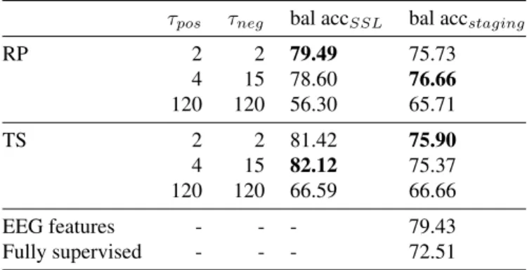
We first evaluate the ability of the CNN architecture to learn on the SSL tasks (see Table 2). We train the feature extractor h on the entire training set using the RP and TS tasks with three sets of hyperparameters τposand τneg. Once h is trained, we

project the labeled samples into the networks’ respective fea-ture space and then train multinomial linear logistic regression models on each set of features to predict sleep stages.

On MASS, τpos = 2, τneg = 2 (in minutes) and τpos =

4, τneg = 15 both led to similar performances on the SSL

and downstream tasks. Making the task harder by using a large positive context (τpos = 120) however led to lower

performance on both SSL and sleep staging tasks. The same conclusion was reached on Sleep EDF (results not shown). We decided to use τpos= 4 and τneg= 15 in our experiments, as

this also increases the number of windows that can be sampled from the positive context.

While these results are a few points below those of a linear classifier trained on common handcrafted EEG fea-tures (79.43%), they are slightly better than full supervision (72.51%), showing our approach achieves comparable perfor-mance to standard approaches but without labels or expert knowledge. SSL performance was similar to full supervision or common EEG features on Sleep EDF as well.

3.4.2. Experiment 2: SSL enables sleep staging with limited annotated data

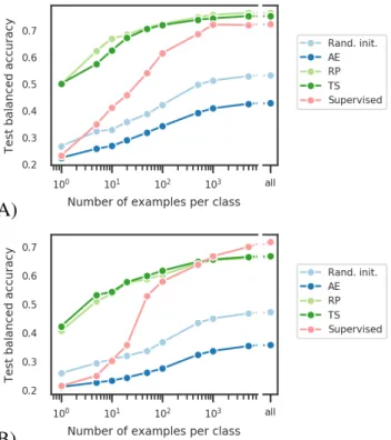
Next, in order to assess whether models trained with SSL can learn informative features, we compare their performance to the performance of various baselines, and explore the effect of varying the quantity of labeled data (see Fig. 1).

Table 2: Test balanced accuracy obtained on the SSL tasks (bal accSSL) and on the sleep staging task (bal accstaging) for

different sets of hyperparameters τposand τneg(in minutes).

Results obtained on MASS.

τpos τneg bal accSSL bal accstaging

RP 2 2 79.49 75.73 4 15 78.60 76.66 120 120 56.30 65.71 TS 2 2 81.42 75.90 4 15 82.12 75.37 120 120 66.59 66.66 EEG features - - - 79.43 Fully supervised - - - 72.51

The feature extractors h are trained using the different ap-proaches (AE, RP and TS on unlabeled data; full supervision on labeled data) and then used to obtain features. We also ex-tract features using models with randomly initialized weights, i.e., that have not been trained. The sleep staging performance is finally evaluated using logistic regression models.

On MASS (Fig.1-A), the SSL features outperformed the purely supervised model for all data regimes, with more than 25 points difference when a single example per class was avail-able. Across most data regimes, RP was found to outperform TS by a fraction of a percent. Finally, both AE and the ran-domly initialized model led to much lower performance, albeit over chance level (∼ 20%). Similar results were obtained on Sleep EDF (Fig.1-B), although the purely supervised model outperformed SSL features above 500 examples per class. TS also led to slightly higher performance than RP.

The model pretrained with an autoencoder obtained very low performance because the reconstruction task, which uses a mean squared error loss, encourages the model to focus on the input signal’s low frequencies. Indeed, these frequencies have higher power than high frequencies in biological signals like EEG. While the autoencoder misses spectral information important for the sleep staging task, the SSL models show relatively high performance.

3.4.3. Experiment 3: SSL models learn physiologically mean-ingful features

To further explore the features learned with SSL, we project the 100-dimension embeddings obtained on the labeled Sleep EDF dataset to two dimensions using UMAP [20]. We use Sleep EDF as it contains subject metadata such as age.

In Fig. 2-A, we notice the emergence of a distinct structure that closely follows the different sleep stages. Indeed, as seen by color-coding samples using their labels, clear groups emerge that not only correspond to the labeled sleep stages, but that are also sequentially arranged: starting from the right

A)

B)

Fig. 1: Impact of number of labeled examples per task on sleep staging performance for feature extractors trained with an autoencoder (AE), the relative positioning (RP) and the temporal shuffling (TS) tasks, a fully supervised model, and a randomly initialized model, (A) on MASS and (B) on Sleep EDF. “All” means all available training examples were used. While higher numbers of labeled examples lead to better per-formance, SSL models achieve much higher performance as supervised models when few examples are available.

of the figure and moving to the left, we can draw a trajectory that passes through W, N1, N2 and N3 sequentially. Stage R, finally, overlaps with W and N1.

Moreover, in Fig. 2-B, one can observe that the embedding encodes age-related information. Samples from younger sub-jects occupy the left outer part of the cloud of points, while samples from older subjects are found in the inner part of the U-shaped structure. This phenomenon is visible in stages N1, N2 and N3 but not in W and R, where no apparent age-dependent structure is visible. This might be explained by the prevalence of sleep spindles, major features used to identify N2 and N3, which are known to change with age [21].

4. DISCUSSION

We introduced two self-supervised learning tasks, relative po-sitioning and temporal shuffling, which we used to learn rep-resentations from electroencephalography (EEG) multivariate time series. Our approach achieves similar performance as

su-A)

B)

Fig. 2: UMAP visualization of temporal shuffling (TS) fea-tures on the whole Sleep EDF dataset. Each point corresponds to the features extracted from a 30-s window of EEG. (A) Sam-ples are color-coded by sleep stage. (B) SamSam-ples for stages N1, N2 and N3 are color-coded by age group while other stages are in grey. As seen from their gradient-like structure, the features encode physiologically relevant information although no labels were available during training.

pervised approaches when tested on a clinically relevant sleep staging task, and largely outperforms a purely supervised ap-proach in lower data regimes. The representation learned with these tasks also encodes physiologically interesting structure such as sleep stages and age, demonstrating their potential to uncover meaningful latent structure in unlabeled data.

While both the SSL tasks proposed were shown to be use-ful for unsupervised training of feature extractors and achieved very similar performance, RP required fewer computations as its implementation uses only two siamese subnetworks, in-stead of three. It might therefore be a better choice thanks to its relative simplicity. The quality of the representation obtained with the RP task as well as its training efficiency could be further improved by 1) modifying the contrastive module g to compute other aggregates of the features (e.g., sum or dot

product) and 2) by using mining strategies, by which tuples are not sampled uniformly but rather based on a predefined criterion. Indeed, the number of training examples (i.e., tuples of two or three windows) available to the RP and TS tasks can be made very high as the number of possible tuples increases exponentially with the number of available windows, which also increases training time. Mining most useful examples could therefore speed up model training.

By reducing the number of labeled data required to reach high performance, the proposed SSL tasks are promising alter-natives to an expensive and time-consuming labeling process, as well as expert handcrafting of task-specific features. Future work will focus on evaluating the usefulness of the SSL task for other types of neural time series recordings, and on assessing the impact of architecture variations and mining strategies.

5. REFERENCES

[1] T.-Y. Lin, M. Maire, S. Belongie, J. Hays, P. Perona, D. Ramanan, P. Dollár, and C. L. Zitnick, “Microsoft COCO: Common objects in context,” in ECCV. Springer, 2014, pp. 740–755.

[2] V. Panayotov, G. Chen, D. Povey, and S. Khudanpur, “Librispeech: an ASR corpus based on public domain audio books,” in ICASSP. IEEE, 2015, pp. 5206–5210. [3] L. Jing and Y. Tian, “Self-supervised visual feature

learning with deep neural networks: A survey,” arXiv preprint arXiv:1902.06162, 2019.

[4] C. Doersch, A. Gupta, and A. A. Efros, “Unsupervised visual representation learning by context prediction,” in ICCV, 2015, pp. 1422–1430.

[5] I. Misra, C. L. Zitnick, and M. Hebert, “Shuffle and learn: unsupervised learning using temporal order verification,” in ECCV. Springer, 2016, pp. 527–544.

[6] A. v. d. Oord, Y. Li, and O. Vinyals, “Representa-tion learning with contrastive predictive coding,” arXiv preprint arXiv:1807.03748, 2018.

[7] A. Hyvärinen and H. Morioka, “Nonlinear ICA of tem-porally dependent stationary sources,” in AISTATS, 2017. [8] A. Hyvärinen, H. Sasaki, and R. E. Turner, “Nonlinear

ICA using auxiliary variables and generalized contrastive learning,” in AISTATS, 2019.

[9] M. Younes, “The case for using digital EEG analysis in clinical sleep medicine,” Sleep Science and Practice, vol. 1, no. 1, pp. 2, 2017.

[10] B. Kemp, A. H. Zwinderman, B. Tuk, H. A. Kamphuisen, and J. J. Oberye, “Analysis of a sleep-dependent neuronal feedback loop: the slow-wave microcontinuity of the

EEG,” IEEE Trans on Biomed Eng, vol. 47, no. 9, pp. 1185–1194, 2000.

[11] A. L. Goldberger, L. A. Amaral, L. Glass, J. M. Haus-dorff, P. C. Ivanov, R. G. Mark, J. E. Mietus, G. B. Moody, C.-K. Peng, and H. E. Stanley, “PhysioBank, PhysioToolkit, and PhysioNet: components of a new research resource for complex physiologic signals,” Cir-culation, vol. 101, no. 23, pp. e215–e220, 2000. [12] R. B. Berry, R. Brooks, C. E. Gamaldo, S. M.

Hard-ing, C. L. Marcus, B. V. Vaughn, et al., “The AASM manual for the scoring of sleep and associated events,” Rules, Terminology and Technical Specifications, Ameri-can Academy of Sleep Medicine, vol. 176, 2012. [13] C. O’Reilly, N. Gosselin, J. Carrier, and T. Nielsen,

“Montreal Archive of Sleep Studies: an open-access source for instrument benchmarking and exploratory re-search,” Journal of Sleep Research, vol. 23, no. 6, pp. 628–635, 2014.

[14] S. Chambon, M. N. Galtier, P. J. Arnal, G. Wainrib, and A. Gramfort, “A deep learning architecture for temporal sleep stage classification using multivariate and multi-modal time series,” IEEE Trans Neur Syst Rehab Eng, vol. 26, no. 4, pp. 758–769, 2018.

[15] D. P. Kingma and J. Ba, “Adam: A method for stochastic optimization,” arXiv preprint arXiv:1412.6980, 2014. [16] J. Masci, U. Meier, D. Cire¸san, and J. Schmidhuber,

“Stacked convolutional auto-encoders for hierarchical fea-ture extraction,” in ICANN. Springer, 2011, pp. 52–59. [17] A. Paszke, S. Gross, S. Chintala, G. Chanan, E. Yang,

Z. DeVito, Z. Lin, A. Desmaison, L. Antiga, and A. Lerer, “Automatic differentiation in PyTorch,” in NIPS, 2017. [18] F. Pedregosa, G. Varoquaux, A. Gramfort, V. Michel,

B. Thirion, O. Grisel, M. Blondel, P. Prettenhofer, R. Weiss, V. Dubourg, et al., “Scikit-learn: Machine learning in Python,” Journal of Machine Learning Re-search, vol. 12, no. Oct, pp. 2825–2830, 2011.

[19] K. Aboalayon, M. Faezipour, W. Almuhammadi, and S. Moslehpour, “Sleep stage classification using EEG signal analysis: a comprehensive survey and new investi-gation,” Entropy, vol. 18, no. 9, pp. 272, 2016.

[20] L. McInnes, J. Healy, and J. Melville, “Umap: Uniform manifold approximation and projection for dimension reduction,” arXiv preprint arXiv:1802.03426, 2018. [21] S. Purcell, D. Manoach, C. Demanuele, B. Cade, S.

Mar-iani, R. Cox, G. Panagiotaropoulou, R. Saxena, J. Pan, J. Smoller, et al., “Characterizing sleep spindles in 11,630 individuals from the national sleep research resource,” Nature communications, vol. 8, pp. 15930, 2017.