HAL Id: hal-01399371
https://hal.archives-ouvertes.fr/hal-01399371
Submitted on 18 Nov 2016
HAL is a multi-disciplinary open access
archive for the deposit and dissemination of
sci-entific research documents, whether they are
pub-lished or not. The documents may come from
teaching and research institutions in France or
abroad, or from public or private research centers.
L’archive ouverte pluridisciplinaire HAL, est
destinée au dépôt et à la diffusion de documents
scientifiques de niveau recherche, publiés ou non,
émanant des établissements d’enseignement et de
recherche français ou étrangers, des laboratoires
publics ou privés.
Phrase table pruning for Statistical Machine Translation
Esther Galbrun
To cite this version:
Esther Galbrun. Phrase table pruning for Statistical Machine Translation. [Technical Report]
C-2009-22, University of Helsinki. 2009, pp.38. �hal-01399371�
Department of Computer Science Series of Publications C
Report C-2009-22
Phrase table pruning
for Statistical Machine Translation
Esther Galbrun
University of Helsinki Finland
Phrase table pruning for Statistical Machine Translation
Esther Galbrun
Department of Computer Science
P.O. Box 68, FIN-00014 University of Helsinki, Finland [email protected]
Technical report, Series of Publications C, Report C-2009-22 Helsinki, July 2009, 38 pages
Abstract
Phrase-Based Statistical Machine Translation systems model the translation process using pairs of corresponding sequences of words extracted from parallel corpora. These biphrases are stored in phrase tables that typically contain several millions such entries, making it difficult to assess their quality without going to the end of the translation process. Our work is based on the examplifying study of phrase tables generated from the Europarl data, from French to English. We give some statistical information about the biphrases contained in the phrase table, evaluate the coverage of previously unseen sentences and analyse the effects of pruning on the translation.
Computing Reviews (1998) Categories and Subject Descriptors: I.2.6 Learning
I.2.7 Natural Language Processing
General Terms: Machine translation
Additional Key Words and Phrases:
Contents
1 Introduction 1 2 Preliminaries 2 2.1 Machine Translation . . . 2 2.1.1 Goals . . . 2 2.1.2 Brief history . . . 2 2.1.3 Approaches . . . 32.2 Phrase-Based Statistical Machine Translation . . . 4
2.2.1 System architecture . . . 4
2.2.2 Data sources . . . 6
2.2.3 Translation evaluation . . . 6
3 Background informations on phrase tables 7 3.1 Motivation . . . 7
3.2 Phrase table generation process . . . 7
3.2.1 Using GIZA++ . . . 8
3.2.2 Using MMBT . . . 8
3.3 Related work . . . 9
3.3.1 Phrase alignment and extraction . . . 9
3.3.2 Alignment quality . . . 10
4 Phrase table experiments 11 4.1 Material . . . 11
4.2 Phrase table features . . . 11
4.2.1 Moses features . . . 12
4.2.2 Sinuhe features . . . 12
4.2.3 MMBT features . . . 13
4.3 Further phrase table characteristics . . . 14
4.3.1 Size of the phrase tables . . . 14
4.3.2 GIZA++ characteristics . . . 14
4.3.3 MMBT characteristics . . . 18
4.4 Phrase table coverage . . . 20
4.4.1 Experiment description . . . 20
4.4.2 Results . . . 22
4.5 Tail cutting, translation quality and speed . . . 25
4.5.1 Sinuhe pruning . . . 26
4.5.2 Tail of candidates . . . 27
4.5.3 Effects of the tail of candidates . . . 29
5 Conclusions 35
Chapter 1
Introduction
The aim of Machine Translation is to automatically translate sentences from a given language into another. Phrase-Based Statistical Machine Translation systems, one approach to solve this problem, use pairs of corresponding sequences of words in the source and target languages to build a probabilistic model of the translation process.
Extracting pairs of corresponding phrases together with their word to word links, the biphrases, from sentence aligned bilingual corpora using statistical and heuristic models to compute the word alignments and storing them in a phrase table is the first step to set such a translation system up. When no intermediate evaluation is available, the full training procedure of the translation system has to be completed before any evaluation can be conducted. The complete loop often requires several days to be carried out, making incremental improvements impractical. Besides the phrase table, many factors are involved in training the system and generating the translations. Thus, in the absence of intermediate evaluation, determining which part of the system is at fault when the translation quality is unsatisfactory can also be challenging.
Therefore, after acquiring a better undertanding of what phrase tables actually contain by computing statistics about the basic characteristics of the biphrases (phrase length, number of occurrences, etc.), we would like to find a way to evaluate their intrinsic quality. Since they typically contain several millions of entries, a manual evaluation by browsing through the biphrases is simply unfeasible. For this reason, we try to estimate the ability of the phrase table to cover previously unseen sentences, without making any assumption on the system that uses them. We want to determine whether the biphrases needed to construct the translations are present in the phrase table, regardless of how the system can combine them.
Finally, we investigate how manipulating the phrase table by filtering out some of the biphrases impacts the translation. We consider the effects of different pruning methods on the translation quality as well as on the size of the model and the translation speed.
The work reported here is based on the examplifying study of translation from French to English, using distinct subsets from the Europarl corpus to train and evaluate the systems.
After giving a overview of the field of Machine Translation in general and of Phrase-Based Statistical Machine Translation more specifically in Chapter 2, we focus on the phrase tables, explaining how they are generated and briefly reviewing related work in Chapter 3. Chapter 4 describes our experimental settings and the results obtained. Chapter 5 concludes this work.
Chapter 2
Preliminaries
2.1 Machine Translation
After defining the main goals of Machine Translation (MT), we briefly present the history of this field. Next, we outline the main approaches that have been used in solving this problem.
2.1.1 Goals
Machine Translation aims at translating sentences from a source language X to a target language Y . The ultimate goal for MT would be to obtain perfect translations, i.e. translations that could not be discriminated from human translations. Yet, this still seems to be too high a target.
There are two main purposes for machine translation outputs, assimilation and dissemination. When used for assimilation purposes, the translation should help the reader in understanding texts originally available in a language he does not read. On the other hand, when used for dissemination purposes, the output is typically post-processed by a human translator in order to obtain high quality translation to be published.
In the case of assimilation the main objective is to retain as much as possible from the original meaning of the text while in the case of dissemination it should output sentences that require minimal post-editing before being acceptable translations for the original sentences. Of course, these two objectives are closely related. A perfect translation would reflect the original content and would not need any edition. But while redundant translations of some difficult words might help to understand the meaning of the translation it would only slow down the post-editing.
MT systems can also be used as part of larger systems. For example, they can be used in cross-lingual information retrieval or for automatic speech processing. In those cases, again, as the end-use changes, the way of characterizing a good candidate translation also varies.
2.1.2 Brief history
A detailed history of MT can be found in [20]. Only the main steps are reported here.
Long before computers became available did intellectuals envision the use of machines to trans-late from one language into another. Shortly after the Second World War, Warren Weaver [36] suggested that some of the innovations made during the war in the field of cryptography could be applied to MT. He compared translating a text from chinese into english to deciphering some encrypted text, the cipher being chinese language. In the 50’s and 60’s, the first attemps to make the old dream of automatic translation become true, resorting mainly to rule-based systems, failed to fulfill the high expectations they had generated. Bar-Hillel, one of the first MT researchers, concluded in 1960 in his review [6] that the objective of producing automatic translations undis-tinguishable from human translations is unrealistic and had to be abandonned. In 1966, a report published by the Automatic Language Processing Advisory Committee (ALPAC) in the United States presented MT as a failure and put an end to almost all research in the field [18]. In the 80’s,
some operational systems were released and attracted back attention. Systran [33] is probably the most famous of them. From the late 80’s, as more resources became available, approaches based on corpora - exemple-based and statistical MT - started to be developed. The latter in particular keeps attracting increasing attention as the amount of data available to feed to those systems continues to grow.
2.1.3 Approaches
We will now introduce the main approaches for solving the problem of Machine Translation.
Expert systems
The first operational MT systems were Rule-Based systems. Such systems use bilingual dictionaries and a large set of rules that are automatically applied to generate a translation. Generally the set of rules needs to be written by a linguist for each specific pair of languages. Alternatively, an artificial representation, an interlingua, can be used as a universal intermediate representation of the semantic content.
Data-driven systems
Example-Based and statistical MT systems both rely on bilingual corpora. But while the former generates translations based on analogies retrieved from the parallel texts at runtime [19], the latter requires a training step to carry out a statistical analysis of the corpora in order to extract relevant knowledge to be used while translating.
Statistical systems Statistical Machine Translation (SMT) [24] uses a probabilistic represen-tation of natural languages and the translation process. To all possible pairs of source language sentence x and target language sentence y is associated a value P r(y|x). This value represents the probability that given the sentence x a translator would choose y as its translation. The best translation given a sentence x is then defined as the sentence ˆy that maximizes P r(y|x). Using Bayes’ theorem this can be rewritten as
P r(y|x) = P r(y)P r(x|y) P r(x) .
For a given source sentence the denominator is constant. Therefore the sentence
ˆ
y = arg max
y
P r(x|y)P r(y)
is the best translation for the source sentence x.
P r(y) models the probability that the sentence y is a valid sentence in the target language, while P r(y|x) models the probability that y is a good translation for x. The former model is called the language model, the latter is the translation model.
The most common language models are based on counts of occurrences of sequences of n successive words, the n-grams, in large monolingual texts.
• Phrase-Based and Syntax-Based SMT
The knowledge extracted from the bilingual corpora in SMT systems to model the translation probabilities can take different forms. It can be syntactic rules, typically represented as operations on parse trees [14], in the case of Syntax-Based SMT, or pairs of corresponding sequences of words in the source and target languages, aligned phrases, in the case of Phrase-Based SMT. The extracted sequences of words in the source and target languages may have varying size. This should take care of fertility issues, i.e., the fact that a word in language may not be translated into exactly one word in the other language. This should also alleviate the problem of reorderings, i.e., the fact that the words in the target language do not necessarily
appear in the same order as the source words they translate and may need to be reordered. However, it cannot entirely solve this issue since the length of the extracted phrases is limited and cannot cover sentence wide reorderings. The set of corresponding sequences of words in the source and target languages is called a phrase table.
• Phrase-Based Machine Translation and Machine Learning
Phrase-Based machine translation can be cast as a machine learning problem. One way of doing so is, for a given input sentence, to predict a label that indicates which phrases appear in the translation and at what position.
2.2 Phrase-Based Statistical Machine Translation
In this section we will present in more detail Phrase-Based Statistical Machine Translation (PB-SMT) systems, in which phrase tables, the object of our interest in this work, are used as the base element to model the translation probability P r(y|x). In the following discussion, we shall distinguish between sentences, the linguistic units of meaning and phrases, sequences of words of varying lengths whose boundaries do not necessarily have a linguistic motivation. A pair of a source language phrase and a target language phrase is called a biphrase and is generally associated with its word to word correspondence relation, called alignment.
2.2.1 System architecture
Here we want to give an overview of the components that make up a Phrase-Based SMT system. As an example, we describe the architecture of Sinuhe translation system [22], one of the systems we studied in this work. In both this system and Moses [17], the system used as a baseline in our work, the phrase table is generated the same way, as described below. However the two translation models use it differently, so the training processes as well as the decoding are different.
Training material
The starting material for Phrase-Based SMT systems is a large bilingual corpus, typically two large texts in the source and target languages which are translations of each other and are aligned at sentence level. Alignment at sentence level means that corresponding lines of the two texts contain sentences that are translations of each other. The bilingual material is separated into a training set, from which the biphrases are extracted and their weights learnt, a tuning set, used to adjust the values of the parameters of the decoder and an evaluation set, to assess the translation quality. A separate monolingual corpus in the target language is needed to train the language model.
Alignment and phrase extraction
Before extracting the aligned biphrases, the training set is tokenized and lowercased. The most common way to perform the phrase extraction is to generate the word to word alignment and then extract the set of biphrases that are compatible with it, called phrase table. The GIZA++ implementation of the IBM models [7] is generally used to perform the word alignment. The IBM models are statistical models of the translation process that are used to evaluate the probabilities of word to word alignements for all pairs of source word and target word given a pair of aligned sentences. There are five models of increasing complexity to take into account effects such as distortion, i.e., the fact that the translations of some words may be swapped, and fertility, i.e., the fact that one word is not always translated into exactly one word in the other language. The parameter values estimated for one model are used as initial values for the next estimation. To obtain a good quality word alignment a series of successive estimations is needed. This iterative process generally requires several hours to be carried out for roughly one million sentences. The models allow one word of a target sentence to be linked to only one word of the source language. To by-pass this constraint, the word alignments are computed in both directions, from source to
target and target to source, and the results are combined as a final step called symmetrization. The result of this alignment process is for each pair of training sentences a set of links between the source words and the target words. An example is given below where x is a source sentence, y a target sentence, and a their word to word alignment, i.e., a set of link between the words of x and y. For example the link 3 − 2 indicates that the fourth word of x, meme is aligned with the third word of y, also.
x: je me permettrai meme , bien qu’ ils soient [...] y: i would also like , although they are absent [...] a: 0-0 1-1 3-2 2-3 4-4 5-5 6-5 7-6 8-7 9-8 10-9 [...]
A biphrase (x0, a0, y0), where x0 is a source phrase, y0 a target phrase and a0 the alignment between the words of x0 and y0 induced by a is considered valid if it contains links but none of them crosses the boundaries of the biphrase. All valid biphrases are stored in a phrase table, along with their count of occurrences.
Learning
From this point Sinuhe and Moses differ in the use they make from the extracted biphrases to model the translation probabilities.
In Sinuhe the biphrases are used to construct φ(x, a, y), a vector indicating which biphrases occurs in (x, a, y), a pair of aligned sentences x and y and their word to word alignment a. More precisely φ(x, a, y)i,j indicates whether the ithbiphrase of the phrase table occurs at position j of
the source sentence. Then ˜φ(x, a, y)iis defined as ˜φ(x, a, y)i=Pj=Jφ(x, a, y)i,j, so it is the count
of occurrences of the ithbiphrase in (x, a, y) over the set of all starting positions J .
The translation model in Sinuhe doesn’t estimate the translation probability distribution P r(y|x) directly but P r(φ(x, a, y)|x) instead, using the features ˜φ(x, a, y) to build a conditional exponential model
P r(φ(x, a, y)|x) = exp(w. ˜φ(x, a, y)) P
˜
φ∈Φxexp(w · ˜φ)
,
where Φxrepresents the set of all possible candidates for the sentence x. The maximum a posteriori
(MAP) [31] estimates of the weights for the biphrases features wi are computed using stochastic
gradient ascent, where the gradients are computed by dynamic programming. The counts of occurrences associated to the biphrases can be used at this stage to compute regularization terms for the weights. Biphrases with unaligned end words are discarded from the phrase table as they cannot be handled by the dynamic procedure, as well as all biphrases occurring only once to prevent overfitting the training data. Since the weights are learnt from the same corpus as the features have been extracted from, if no pruning was applied to the phrase table prior to the learning phase, the system could simply use all the biphrases that were extracted from an aligned pair of sentences to reconstruct it.
Decoding
Decoding is the dynamic procedure of finding the translation that maximizes the translation prob-ability. Once the weights have been learnt, the translation can be generated by selecting the vector ˜
φ(x, a, y)ithat receives the highest translation model probability and reconstructing the translation
induced by the target side of the biphrases active in that vector.
Alternatively, additional scores can be taken into account to select the best candidate transla-tion:
• a language model score, given by an external language model trained separately, • a word level lexical translation probability,
• a distortion score, to penalize for reorderings in the translation.
The contribution of the different scores in the decoding is tuned using Minimum Error Rate Train-ing (MERT) to optimize the BLEU score (cf. 2.2.3) on the tunTrain-ing corpus.
2.2.2 Data sources
As we mentioned, bilingual corpora are the starting material for SMT systems.
Since the Canadian Government is officially bilingual, the proceedings of the Canadian Par-lament have to be maintained both in French and English. Likewise, the European Parliament also maintains proceedings in the official languages of its member states. The proceedings of these two political institutions, the Canadian Hansard [27] and the Europarl [23, 12] respectively, have traditionally been the most important resources for Statistical Machine Translation between Eu-ropean languages. A major inconvenience of these two sources arises from the fact that they are parliament proceedings. They have a very specific focus and contain many atypical formulations that are not useful to translate texts from other domains.
A new French-English corpus generated by automatically crawling bilingual websites has re-cently been released for the translation task of the fourth European Chapter of the Association for Computational Linguistics (EACL) Workshop on Machine Translation (WMT09). This Giga French-English [12] corpus contains over 20 millions sentences in both languages, to be compared to Europarl corpora of typically slightly more than 1 million sentences.
Finding training material is a crucial point in developing a SMT system for a new language pair. For some language pairs, in particular those that involve rare languages, finding aligned bilingual texts can be really challenging. Therefore, some alternative approaches have been developed to take advantage of texts that are similar but not exact translations of each other [29] or even from two monolingual datasets [16], or to use a third language as an intermediate [37].
2.2.3 Translation evaluation
Evaluation of translation systems output is a hard, tedious and highly subjective task. Common criteria are fluency and adequacy. Fluency indicates whether the translation is a correct sentence in the target language and can possibly be evaluated by a person who only reads the target language. Adequacy measures how well the original meaning was conveyed to the translation and needs to be evaluated by a bilingual person.
Automatic evaluation tools are required not only to compare systems but also during the training process since systems are often trained to optimize a criteria on the translation quality. Various metrics have been developed to approximate human judgment. They generally require human reference translations of the test sentences to be at hand. The most widely used metric for evaluating machine translation output is the BLEU score [28]. This score is based on n-grams precision evaluation. The basic idea is to count how many n-grams from the candidate translation are present in the reference. This might seem a coarse criterion for evaluation and its use is subject to much critisism. But while much research effort has been directed toward inventing metrics that correlate better with human judgement [3, 8, 38], no satisfactory solution has been developed. The very existence of an automatic tool for evaluating the quality of such complex objects as instances of natural language is arguable. There are for example many different ways to translate the same idea that might be acceptable. Using several references has been shown to increase the reliability of the evaluation [34]. There is also much discussion about how to evaluate the quality of candidate translations when no reference is available. This is needed in particular to rank several candidate translations generated by one or different systems.
Automatic Machine Translation evaluation remains a difficult task. The use of multiple metrics has been recommended but it can be computationally heavy and the results may be difficult to interpret so that BLEU score alone still is widely used despite its evident flaws.
Chapter 3
Background informations on
phrase tables
3.1 Motivation
Phrase tables are corner stones of Phrase-Based Statistical Machine Translation systems. Therefore the phrase table quality is critical in the overall quality of the translation system. The quantity of biphrases in the model is also a very important factor determining the size of the model and the speed of the learning and of the translation processes.
We focus here on three systems:
• Moses, a state-of-the-art open-source toolkit [17] for Statistical Machine Translation, is usu-ally used as a baseline in Phrase-Based SMT.
• A SMT software that models the translation probabilities using a conditional exponential family, Sinuhe [22].
• An application of multiview learning to machine translation, based on the maximum margin regression algorithm [32], the Maximum Margin Based Translator (MMBT).
Both Sinuhe and MMBT where developed for the SMART EU project [30].
We want to consider more closely the phrase tables used by those three systems. Moses and Sinuhe both rely on the GIZA++ implementation of the IBM models [7] to generate the word align-ments but the biphrases extracted after symmetrization are scored and filtered differently. MMBT has its own alignment, biphrases extraction and scoring algorithm. We will analyse theses three different phrase tables, trying to get a better understanding of what they contain and looking for patterns that would enable us to discriminate between good and bad biphrases. If such charac-teristics were found, we could in particular reduce the search space during the decoding process, without affecting significantly the quality of the final translation.
What we call good biphrases are pairs of source and target phrases that are correct translation of each other, have proper boundaries and valid weights. We would also like to find a compromise for the size of the model. On one hand, an important part of large phrase tables may be constituted of biphrases which are very specific to the training corpus and rarely occur in texts to translate. On the other hand, small phrase tables that contain only frequent expressions may be unable to translate constructs slightly out of the ordinary.
3.2 Phrase table generation process
In this section, we describe how the phrase table is generated from the sentence aligned training corpus. First for Moses and Sinuhe translation systems starting from word alignments generated using GIZA++, then with MMBT.
3.2.1 Using GIZA++
Most of the current Phrase-Based SMT systems rely on the GIZA++ implementation of the IBM Models [7] to produce word alignments, running the algorithm in both directions, source to target and target to source. Various heuristics can then be applied to obtain a symmetrized alignment a from those two. Most of them, such as grow-diag-final-and, that we used, start from the intersection of the two word alignment and enrich it with alignment points from the union. Word sequences are then stored in the phrase table as biphrases (x0, y0) along with their alignment a0 if they satisfy the following conditions:
1. x0 and y0 are consecutive word subsequences in the source sentence x and target sentences y respectively and neither of them is longer than k words.
2. a0, the alignment between the words of x0 and y0induced by a, contains at least one link and all links from a have either both ends in a0 or none.
Moses phrase table
Moses uses directly the biphrases extracted from the GIZA++ word aligments without any further processing apart from the scoring explained in 4.2.1.
Sinuhe phrase table
Sinuhe does not use the full phrase table obtained from the GIZA++ word aligments. After associ-ating count-based features to the biphrases as presented in 4.2.2, before proceeding to the learning of the biphrases’s weights, the phrase table is pruned by filtering out biphrases that satisfiy any of the six following criteria:
1. single occurrence, the pair (source phrase, target phrase) occurs only once in the corpus,
2. rank, the biphrase is not among the N most frequent among all biphrases sharing the same source phrase (N is typically fixed to 20),
3. first source word unaligned, the first word of the source phrase is not aligned to any word on the target side,
4. last source word unaligned, similarily the last word of the source phrase is not aligned to any word on the target side,
5. first source word unaligned, and
6. last source word unaligned, similar to 3. and 4. with respect to the target phrase.
The motivation for removing biphrases that occur once is to avoid overfitting the training data by leaving out biphrases that are specific to that corpus and are unlikely to occur anywhere else. Having only biphrases whose first and last word are aligned simplifies the learning of feature weights [22]. Biphrases farther than the twentieth are likely to be assigned too low probabilities compared to the most frequent ones to be actually used in translations.
3.2.2 Using MMBT
MMBT is an application of multiview learning to machine translation. It predicts an ouput label associated to some given input features. A detailed explanation of the method can be found in [30].
Machine Translation deals with how to arrange words into sentences. Therefore, the inputs are features associated to words, both from the target language and source language. They are similarity measures, representing how closely two words are related to each other, based on how often they occur in the training data at neighboring positions. To a word w is associated a vector
φSs,St(w) representing how closely w relates to the words in the source sentence Ss and in the
target sentence St.
Consider a sentence S and a set of phrases P1, P2, . . . , Pn that cover it. The label to predict
for a word w is a binary vector indicating which phrases w belongs to ψ(w)S = (w ∈ P1, w ∈
P2, . . . w ∈ Pn).
Once these representations have been fixed, the learning problem is can be defined as follows:
min1 2 k W k 2 F robenius+C nSs X k=1 ξk, (3.1)
w.r.t. W linear operator, ξ loss,
s.t. hψSs(wk), W φSs,St(wk)i ≥ 1 − ξk, wk ∈ Ss,
ξ ≥ 0 and C > 0 penalty constant.
When W has been computed, here assuming that the source words are the training set, the label for a target word wlis W φSs,St(wl). This vector does not contain boolean indicators but real
values. The strength of the relation between a source word wk and a target word wl can then be
computed as R(wk, wl) = hψSs(wk), W φSs,St(wl)i.
Two such closeness matrices are computed, considering the source words as the training set and computing the labels for the target words as well as in the other direction and summed. The result is a nSs × nSt matrix, D, where nSs and nSt are the number of words in the source and target
sentences respectively. D(i, j) measures how closely the ithword of the source sentence relates to
the jth word of the target sentence.
The next step is to extract biphrases from this matrix. Consider a source phrase of length k starting at position i of St, i.e., some adjacent lines of D with indices [i, i + k − 1]. The aim of
the phrase extraction process is to find the target phrase that gives the best match, i.e., the set of adjacent columns of D with indices [j, j + k0− 1] such that the similarity is maximized in the window defined by the indices and minimized outside.
The extraction is done using the following heuristic. Only values that are row or column maxima are kept. For a source phrase, all target words that are aligned to some source word are collected. Words whose score is below a certain threshold are removed and the remaining ones sorted in the order of the target sentence. The obtained biphrase is stored in the phrase table if it does not contain more than a one word gap and its target phrase length does not differ from that of the source phrase by more than one word.
3.3 Related work
3.3.1 Phrase alignment and extraction
Extracting aligned biphrases from the symmetrized word alignments generated using the IBM models, as presented in 2.2.1, is by far the most widely used technique to generate the phrase table. Alternative methods have been proposed to directly generate the phrase level alignment using statistical models [26], with a machine learning approach as in MMBT (described in 3.2.2) or using integer linear programming [11]. The model proposed in [25] refines the IBM models by adding agreement constraints between the alignments in direct and reverse direction, leading to improved final word alignments.
Starting from the word alignments generated by the IBM models in both directions, various symmetrization and extraction heuristics can be applied. Different criteria have been studied to discard some biphrases from the phrase table, based on usage statistics [13] or significance tests [21]. The latter reported no decrease in BLEU score while removing up to 90% of the biphrases. The use a Gibbs sampler initializied with the IBM word alignments to estimate biphrases frequencies is proposed in [10]. These weights were shown to allow for a better use of the phrases.
A filtering technique using triangulation with a bridge language is presented in [9]. Given an original phrase table PX,Y to be pruned, between languages X and Y and the two phrase tables
(x, y) from the original phrase table to be kept, there must be a phrase z in the third language such that (x, z) ∈ PX,Z and (z, y) ∈ PZ,Y. This approach is claimed to yield increased BLEU score up
to 2.3 points, depending on the language used as a bridge. Nevertheless, applying this technique requires to obtain the bridge phrase tables PX,Z and PZ,Y, meaning that aligned corpora in the
language pairs (X, Z) and (Z, Y ) have to be at hand and two additional alignment processes run.
3.3.2 Alignment quality
Precision, Recall and Alignement Error Rate (AER) are generally used to evaluate the quality of word alignments. A reference alignment is required to use these metrics. Reference alignments are definied manually and contain two kinds of links, sure (S) and probable (P), with P ⊆ S, to which the links (A) of the studied alignment are to be compared. The metrics are then defined as follows: P recision =| A ∩ P | | A | , Recall = | A ∩ S | | S | , AER = | A ∩ S | + | A ∩ S | | A | + | S | .
The impact of word alignment quality on the final translation has been studied [35, 5, 15], showing that improved AER does not necessarily leads to better translations, in terms of BLEU score in particular. The results presented in [35] suggest that the usage of the biphrases by the decoder should be taken into account when tuning the alignments.
A thorough analysis of the search space of phrase-based systems can be found in [4]. In that work, phrase-based systems are compared to hierachical phrase-based systems, studying the reach-ablity of a set of translations and analysing symptomatic errors.
Chapter 4
Phrase table experiments
4.1 Material
The work we report here was made using a phrase table obtained with GIZA++ to generate the alignment on one side and the MMBT alignment algorithm on the other. The phrase tables have been obtained using the Europarl training data, from French to English, made available for the translation task of the fourth European Chapter of the Association for Computational Linguistics (EACL) Workshop on Machine Translation (WMT09) [23, 12]. europarl-v4.fr-en was tokenized, lowercased and long sentences (over 40 words) filtered out before being used as the training data. We used two sets of 2000 tokenized and lowercased sentences, dev2006 and test2007, as tuning and evaluation data respectively. Statistics of the three datasets are reported in Table 4.1.
Typically, the phrase tables we consider come as ordinary text files containing one line per biphrase, each line having four fields:
source phrase, a short sequence of words as it appears in the source corpus,
target phrase, a short sequence of words as it appears in the target corpus,
alignment, the mapping between the words of the source phrase and the target phrase, and
features, counts, translation probability, etc.
The features assigned to each biphrase depend on the scoring procedure. In the next section, we will present in more detail how the phrase tables are generated from the parallel corpora, what features are associated with them for each of the three different systems studied here, and how we could use them to discriminate the biphrases.
All three translation systems were used as of March 2009. The source code of Moses translation system can be downloaded from [1]. A step by step guide from installation to translation and a detailed manual can be found on the website of the WMT09 [12] where it is used as a baseline. The source code of Sinuhe translation system can be downloaded from [2] and contains installation instructions. The source code of MMBT is not available online but can be obtained from its author.
4.2 Phrase table features
After extracting the biphrases from the aligned corpus, numerical features are associated to them which can be used for a preliminary pruning or in the training phase and decoding. In this section we will present in more detail the different features generated by the three scoring procedures. Two are applied to the GIZA++ alignments, in Moses and Sinuhe respectively and one in the MMBT system.
europarl-v4.fr-en dev2006 test2007 French English French English French English sentences 1050377 2000 2000 words 23812195 21617161 64331 58762 64339 59156
Table 4.1: Statistics of the data
4.2.1 Moses features
Moses phrase table contains five features per biphrase (mosi, i ∈ [1, 5]):
1. the phrase translation probability ϕ(f |e),
2. the lexical weighting lex(f |e),
3. the phrase inverse translation probability ϕ(e|f ),
4. the inverse lexical weighting lex(e|f ),
5. the phrase penalty, currently always e = 2.718.
The first four features are probabilites, so they take values between zero and one. The fifth one, being constant is not used in our experiments. These features are directly used by the decoder.
4.2.2 Sinuhe features
Sinuhe phrase table also contains five features per biphrase (sini, i ∈ [1, 5]):
1. the number of occurrences of the triple (source phrase, target phrase, alignment) in the training data,
2. the number of occurrences of the source phrase,
3. the number of occurrences of the target phrase,
4. the rank of the pair (source phrase, target phrase) among all such pairs sharing the same source phrase,
5. the rank of the pair (source phrase, target phrase) among all such pairs sharing the same target phrase.
These features are not used directly by the decoder but for filtering the phrase table prior to learning and determing the regularization during the weights estimation.
Note that we have the following correspondence between Moses’s features and Sinuhe’s, from the definition of the translation probabilities:
mos1= sin1 sin2 and mos3= sin1 sin3 . (4.1)
Sinuhe’s features, as they are not normalized, are not as easy to handle as Moses’s probabilities but allow for finer distinctions. Let us take some biphrases and consider the scores they are given in Moses and Sinuhe phrase table respectively to illustrate this point. The two lines below are extracted from Moses phrase table, they have very similar scores.
absence de mme ||| absence of mrs ||| (0) (1) (2) ||| (0) (1) (2) ||| 1 0.239303 1 0.0623942 2.718
abstention exprime ||| abstention expresses ||| (0) (1) ||| (0) (1) ||| 1 0.293781 1 0.0659091 2.718
absence de mme ||| absence of mrs ||| 0-0 1-1 2-2 ||| 5 5 5 1 1
abstention exprime ||| abstention expresses ||| 0-0 1-1 ||| 1 1 1 1 1
Both biphrases are scored mos1 = mos3 = 1, because the source and target phrases always
co-occur in the training data, but the first biphrase co-occurs five times, the second only once. As a consequence while the two will be handle in the same way in Moses, with Sinuhe the first will be kept but the second pruned out.
Another example follows, again the first group of biphrases are extracted from Moses’s phrase table and second one from Sinuhe. Here all biphrases have scores mos1 = 0.25 and mos3 = 0.5
since the pair (source phrase, target phrase) occurs with every other occurrence of the source phrase but only every fourth occurrence of the target phrase. Nevertheless, the first biphrase occurs five times in the training data while the last one occurs only once.
abolit ||| abolishes ||| ...
||| 0.25 0.263158 0.5 0.25 2.718 abandonnera ||| will abandon ||| ...
||| 0.25 0.00621805 0.5 0.078478 2.718
adopte par le conseil et ||| adopted by the council and ||| ... ||| 0.25 0.00637363 0.5 0.0748383 2.718
affirmation que l’ ||| insistence that the ||| ... ||| 0.25 0.000199703 0.5 0.000491218 2.718 abolit ||| abolishes ||| ...
||| 5 10 20 1 2
abandonnera ||| will abandon ||| ... ||| 3 6 12 1 1
adopte par le conseil et ||| adopted by the council and ||| ... ||| 2 4 8 1 1
affirmation que l’ ||| insistence that the ||| ... ||| 1 2 4 1 1
The lexical probabilities mos2 and mos3 are the product of the lexical translation probabilities
lex(wf|we) and lex(we|wf) respectively over aligned word-pairs (wf, we) in the biphrase. Thus
they are linked to the number of occurrences of the individual words of the biphrase in the training data and to the length of the biphrase, but they do not give a direct indication of the number of occurrences of the biphrase as a whole.
4.2.3 MMBT features
MMBT phrase table only contains two features per biphrase (mmbti, i ∈ [1, 2]):
1. the number of occurrences of the triple (source phrase, target phrase, alignment) in the training data,
2. the sum of the margins computed for each occurrence.
Figure 4.1 is a plot of the features of the MMBT phrase table, second feature as a function of the first feature, for the biphrases verifying mmbt1< 5000 (includes over 99% of the points).
The points seem to lies along two different lines. Using biphrases such that 1000 < mmbt1 <
5000 to obtain a more reliable estimation from biphrases occurring multiple times, the linear regressions obtained for the two clusters have coefficients close to a1 = 2.886 and a2 = 2.305
respectively. Yet, the lower cluster is more subject to noise. The two affine functions mmbt2 =
a1mmbt1 and mmbt2= a2mmbt1 are displayed on Figure 4.1 in red and green respectively.
As the second feature accumulate the margins when the biphrase occurs multiple times, the two features are clearly linearly dependent. However the existence of two biphrases clusters based on the value of the quotient mmbt2
mmbt1 should be considered to check whether they have different
Figure 4.1: MMBT features, mmbt2 vs. mmbt1 phrase table # biphrases size Moses 46058264 5.9 GB MMBT 1936768 138.5 MB
Table 4.2: Sizes of the phrase tables
4.3 Further phrase table characteristics
In this section we present some characteristics of the phrase tables, trying to identify some that could be used along with their features to discriminate between good and bad biphrases.
4.3.1 Size of the phrase tables
Trained on the same data, the phrase tables obtained using GIZA++ or MMBT have very different sizes.
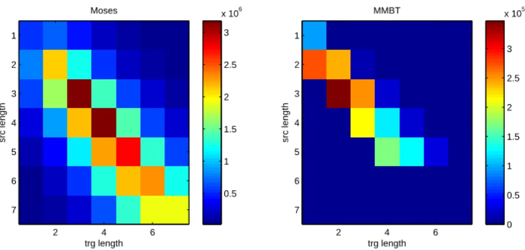
The phrase tables obtained using GIZA++ are about 23 times larger than those obtained with MMBT with respect to the number of biphrases but over 40 times larger with respect to the size of the file on disk as one can see from Table 4.2.
The distribution of biphrases with respect to their source length and target length as a ratio of the whole set of biphrases is shown on Figure 4.2. The GIZA++ algorithm allowed to retrieve phrases up to length 7 on both sides while MMBT was limited to 6. But regardless of that limit, MMBT concentrates much more on shorter biphrases and allows for much less distortion between the lengths on the source and target sides. This observation and the fact that the MMBT phrase table contains only two features per biphrase while Moses’ contains five features probably explains the difference in disk size.
4.3.2 GIZA++ characteristics
Since Moses and Sinuhe both rely on GIZA++ alignment and the same symmetrization heuristic, their characteristics are the same, only the scoring methods vary. Therefore, the results presented in this section are valid for both of them.
trg length src length Moses 2 4 6 1 2 3 4 5 6 7 trg length src length MMBT 2 4 6 1 2 3 4 5 6 7 0.5 1 1.5 2 2.5 3 x 10⁶ 0 0.5 1 1.5 2 2.5 3 x 10⁵
Figure 4.2: Distribution of the biphrases depending on the source length and target length
Pruning criteria
We look at the repartition of the biphrases to the groups made up by the six criteria used by Sinuhe to prune the phrase table. Using the phrase table generated by GIZA++ from the whole Europarl training data and scored by Sinuhe, we extracted every fiftieth biphrase (the whole phrase table is too large to be handled in Matlab).
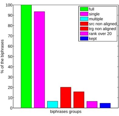
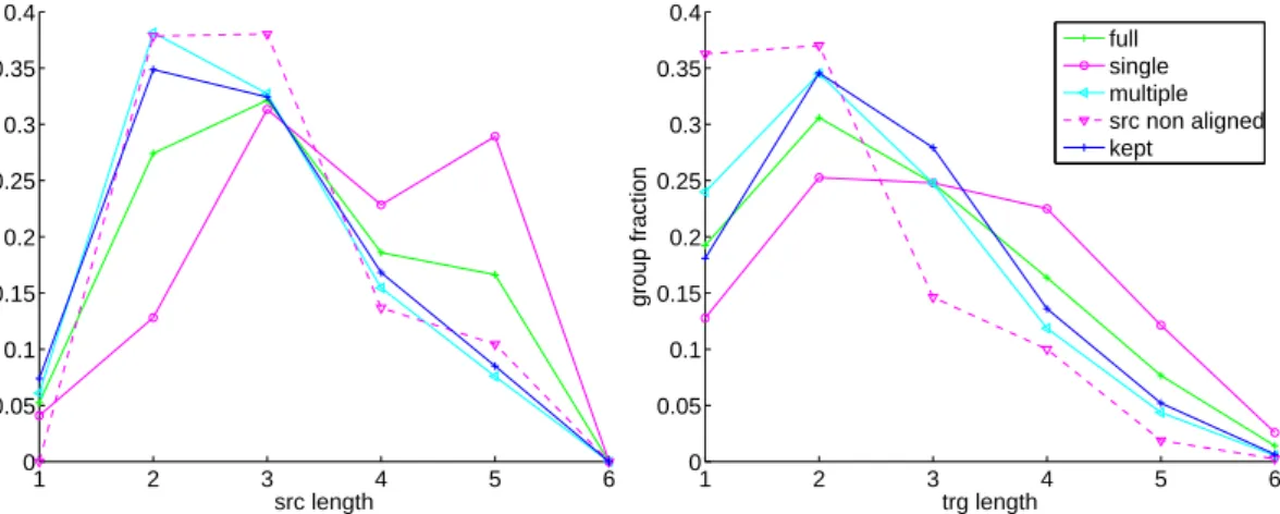
Figure 4.3 shows the number of biphrases contained by the following different groups:
full all extracted biphrases,
single biphrases occurring only once,
multiple biphrases occurring multiple times,
src non aligned biphrases whose first source word, last source word or both are not aligned,
trg non aligned biphrases whose first target word, last target word or both are not aligned,
rank over 20 biphrases that are ranked lower than twenty with regard to the count of occurrences for the same source phrase, and
kept biphrases that are retained in the phrase table after pruning.
Of course, there are overlaps between some of these groups. For example, a biphrase may occur once and have its first source word unaligned. Groups of biphrases that are left out by the pruning process are represented in red/pink while blue/cyan are used for biphrases that are retained in the phrase table.
Over 93% of the biphrases occur only once, about 20% have deficient alignment on their source side and about 16% on their target side. After pruning, only about 4.6% of the biphrases are retained.
The proportion of well-aligned biphrases is significantly higher among multiple-occurring biphrases than among single-occurring ones (76% in the former group, 67% in the latter).
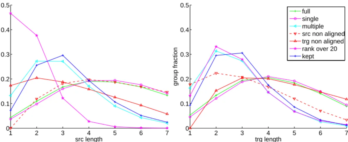
Figure 4.4 and Figure 4.5 show for each of the different groups the distribution of biphrases according to their source or target phrase length and length distortion (i.e., length of the source phrase minus length of the target phrase), respectively.
Phrases lengths
The distributions of biphrases according to their source length or target length in the full phrase table are alike, since the extraction process is symmetrical and does not depend on the direction.
0 10 20 30 40 50 60 70 80 90 100 % of the biphrases biphrases groups full single multiple src non aligned trg non aligned rank over 20 kept
Figure 4.3: Percentage of Sinuhe biphrases in each group
The lengths are very similar to the distribution of n-grams depending on their length n that can be observed in N-gram language models.
The number of different possible n-grams formed using words taken from a dictionary con-taining K words grows exponentially with respect to n since there are K times as many possible combinations of n words as there are combinations of n − 1 words. Nevertheless, kn, the number
of different n-grams actually observed in a corpus does not follow this exponential growth because of syntactic and semantic limitations on the possible combinations in natural languages. This property is the basis of N-gram language models. For n > 4, kn even decreases. Indeed, beyond
four words, there are fewer and fewer distinct phrases that occur in the data because of the data sparsity and sentence boundaries.
The distribution of source length for the biphrases with deficient source alignment is approx-imatetly the same as for the whole phrase table apart that there are no biphrases of length one for which that single word is not aligned. This would yield an empty alignment and this is not allowed during the phrase extraction. The same pattern is repeated on the target side.
Length distortion
The distribution of biphrases depending on the difference between the length of their source phrase and the length of their target phrase is centered on zero with variance around 1.99. This means, as we would expect, that most of the biphrases have equal length on source and target sides. The variance is quite high, some of the biphrases that were retrieved even have for example a source phrase of length one while the target phrase contains the maximum allowed seven words, yielding in this case a negative distortion of 6 words.
Many asymmetric biphrases are obtained by gluing an unaligned word on one end of the phrases, creating an extension with a deficient alignement. Unaligned words preceeding or following well-aligned symmetric biphrases are attached to them, producing asymmetric extensions. For that reason, the distribution of biphrases with unaligned end word on source side and on target side are very similar to the distribution of the complete phrase table with a one word shift toward
1 2 3 4 5 6 7 0 0.1 0.2 0.3 0.4 0.5 src length group fraction 1 2 3 4 5 6 7 0 0.1 0.2 0.3 0.4 0.5 trg length group fraction full single multiple src non aligned trg non aligned rank over 20 kept
Figure 4.4: Distribution of Sinuhe biphrases depending on their length
−4 −2 0 2 4 0 0.1 0.2 0.3 0.4 0.5 0.6 length distortion group fraction full single multiple src non aligned trg non aligned rank over 20 kept
Figure 4.5: Distribution of Sinuhe biphrases depending on their length distortion
source length or target length respectively. Removing biphrases with deficient alignment (33% of the biphrases) reduces the variance in distortion to about 1.29.
Keeping only multiple-occurring biphrases favors shorter phrases, reducing the potential for distortion. As a consequence this further lowers the variance in distortion to 0.78. An asymmetry toward longer biphrases on the source side remains. It is probably due to the fact that French is more wordy than English and French texts are generally longer than their English translation by a few words.
Lox rank biphrases
The last pruning criteria discards biphrases that are ranked lower than twenty among the candi-dates for a given source phrase. Source phrases that have more than twenty candicandi-dates must be very frequent, so as to be extracted along with more than twenty different target phrases. These different target phrases can be generated by different alignments in various sentences or as exten-sions, by gluing unaligned words on one or both sides of the target phrases. For example, the french phrase affaire occurs 3243 times in the training data. It has been extracted with 514 differ-ent target phrases. Among them are 169 single words, 34 well-aligned 2-grams and 2 well-aligned 3-grams, the remaining 309 candidates are extensions with deficient alignment.
# candidates # source phrases 1 1227906 2 118914 3 51493 4 26725 5 41931
Table 4.3: Number of candidate biphrases per source phrase for MMBT
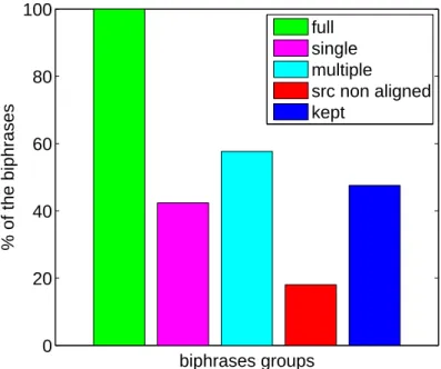
0 20 40 60 80 100 % of the biphrases biphrases groups full single multiple src non aligned kept
Figure 4.6: Percentage of MMBT biphrases in each group
4.3.3 MMBT characteristics
Pruning criteria
To compare the characteristics of the two different phrase tables, we studied the repartition of MMBT biphrases to the goups made up by Sinuhe pruning criteria. Note that as a consequence of the biphrase extraction process there are no biphrases with deficient alignment on the target side, since a target word has to be linked to some word of the candidate source phrase to be retrieved in the candidate target phrase. Therefore, deficient alignments can be found only on the source side. In the phrase table generated using MMBT there were at most five different biphrases for one given source phrase. 86% of the source phrases have only one candidate biphrase, as shown in Table 4.3. The pruning criterion based on rank is therefore not applicable here.
Thus, only five groups are taken into consideration: full, single, multiple, src non aligned and kept. As for Sinuhe’s biphrases, Figure 4.7 and Figure 4.8 show for each of the different groups the distribution of the MMBT’s biphrases according to their source or target phrase length and length distortion (i.e., length of the source phrase minus length of the target phrase) respectively.
Length distortion
As can be seen from Figure 4.2, the alignment obtained with MMBT is strongly biased toward asymmetric biphrases, compared to the one obtained with GIZA++. It retrieves a much larger proportion of biphrases whose source phrase is longer than the corresponding target phrase by one
1 2 3 4 5 6 0 0.05 0.1 0.15 0.2 0.25 0.3 0.35 0.4 src length group fraction 1 2 3 4 5 6 0 0.05 0.1 0.15 0.2 0.25 0.3 0.35 0.4 trg length group fraction full single multiple src non aligned kept
Figure 4.7: Distribution of MMBT biphrases depending on their length
−20 −1 0 1 2 0.2 0.4 0.6 0.8 1 full single multiple src non aligned kept
Figure 4.8: Distribution of MMBT biphrases depending on their length distortion
word.
In fact, the bias toward positive length distortion of the alignment algorithm may even be stronger, producing a large number of biphrases whose source phrase is longer than the corre-sponding target phrase by two or more words. Since only one word distortion is allowed during the extraction such biphrases are filtered out and we cannot assert whether this phenomena really occurs or not.
We also noticed that a gaussian kernel, instead of the default polynomial kernel configuration, produced very symmetrical alignments. However this was only tested for a small corpus and we cannot be certain that this result would generalize to a larger corpus as we were not able to run it on the larger corpus for computational reasons.
Almost all biphrases with unaligned words on the source side are asymmetric, problably pro-duced by extending some aligned biphrase by gluing an unaligned word to its end or beginning.
Applying pruning rules to the phrase table allows to obtain characteristics that are more in line with what we would expect, in terms of symmetry in particular. This is possible only at the expense of a reduction of the phrase table size. Modifying the extraction algorithm and maybe the alignment algorithm might allow to correct this bias and help to further enhance the quality of the phrase table while keeping it at a reasonable size.
By default, a biphrase must occur at least once if the source phrase contains only one word, four times if it contains between two and four words and twice if it contains five or six words. This criteria is responsible for the irregularities in the distribution of source lengths, which is also
closely linked to the distribution of target lengths.
4.4 Phrase table coverage
Our aim with this experiment is to compare how well a test set is covered by the biphrases of the different phrase tables, not making any assumptions on subsequent components such as the decoder or the language model, the capability of the system to handle reorderings, etc. The procedure we followed is explained in more details in the next section before presenting the results we obtained.
4.4.1 Experiment description
Metrics
For this test, we propose to retrieve the biphrases whose source phrase match n-grams in the source test sentence using some feature of the biphrase or a combination of features to threshold the phrase table. We analyse how the bag of words obtained from the biphrases’ words on target side covers the target test sentence using metrics similar to the common precision and recall:
P = inter
sumT and R = inter
sumR , (4.2)
where
inter is the number of words common to the target sentence and the aggregate bag,
sumT is the number of words contained in the aggregate bag (test), and
sumR is the number of words contained in the target sentence seen as a bag of words (reference).
R quantifies how well the test sentences were covered and can be assimilated to a measure of recall, while P quantifies how large a bag of word has been retrieved from the phrase table and can be assimilated to a precision measure. These measures can also be computed so that only the presence of the words, not their number of occurrences, is taken into account.
To evaluate the coverage at corpus level one can either
1. use micro-averaging, denoted with subscript mic, i.e., calculate the total inter, sumT and sumR for all sentences then compute P and R, or
2. use macro-averaging, denoted with subscript mac, i.e., compute P and R for each sentence and then average over all sentences.
Compared with micro-average, macro-average puts more emphasize on the shortest sentences. Nevertheless, the difference between the two measures is only noticeable for the first thresholds and vanishes as the size of the bags of words grows. Later in this report we use micro-average, unless otherwise stated, as it proved to be more stable for the first thresholds.
Outline
To carry out our experiment we follow the outline described below.
• Run the algorithm to obtain a scored phrase table (GIZA++ and Moses or Sinuhe scoring and pruning / MMBT).
• Associate to each biphrase a unique score using some function of the features found in the original phrase table. For that scoring function choose a set of K thresholds, defining bins in which to categorize the biphrases depending on their score, such that they give some nice partition of the biphrases. With Moses, the biphrases are scored using mos1.mos3, the
product of the first feature (direct translation probability) and the third feature (reverse translation probability) of the phrase table (cf.4.2.1). With Sinuhe we used the equivalent
score formula sin1
sin2.sin3, to obtain comparable results (cf. 4.2.2). For MMBT, the score is mmbt2 mmbt1,
the quotient of the second feature by the first feature (count) of the phrase table, i.e., the average margin (cf. 4.2.3).
• Choose a test dataset, an aligned corpus of J sentences.
• For each of the sentences of the source corpus look for all possible n-grams that appear in the phrase table on the source side, with n varying from 1 to a chosen length N , generally the maximum length of the source phrases in the studied phrase table. Split the corresponding target phrase into words. For each score bin, construct a bag containing all target words obtained from phrases whose score fall in that particular bin. There is no order between the words in the bag, but each of the words is associated to its count of occurrences.
• Progressively aggregate the bags from bins with increasing or decreasing thresholds and evaluate how the target sentence is covered at each step using P and R.
More formal definition
Our framework is defined by the following parameters:
• Different algorithms to generate phrase tables are compared: L phrase tables (1 . . . l), • A set of thresholds (t1, t2, . . . tk, . . . ) defines bins, such that the bin k contains biphrases
whose scores s are such that tk− 1 < s <= tk : K bins (1 . . . k),
• An aligned test corpus: J test sentences (1 . . . j),
• All words that appear on the target side, either in the phrase table or test dataset makes up a dictionary containing I words indexed from 1 to i: I words (1 . . . i).
This allows use to define:
• Wt(i, j, k, l), non-negative integer, as the number of times the word i is predicted for the
sentence j, using the bin k of the phrase table l.
• Wr(i, j), non-negative integer, as the number of times the word i appears in the target
sentence j.
• Zt(i, j, k, l), boolean, indicating whether the word i is predicted for the sentence j, using the
bin k of the phrase table l.
• Zr(i, j), boolean, indicating whether the word i appears in the target sentence j.
inter(j, k, l) =X
I
min(Wt(i, j, k, l), Wr(i, j)), (4.3)
sumT (j, k, l) =X I Wt(i, j, k, l), (4.4) sumR(j) =X I Wr(i, j), (4.5) Pmic(k, l) = P Jinter(j, k, l) P JsumT (j, k, l) , (4.6) Pmac(k, l) = 1 J X J inter(j, k, l) sumT (j, k, l), (4.7) Rmic(k, l) = P Jinter(j, k, l) P JsumR(j, k, l) . (4.8)
0 0.2 0.4 0.6 0.8 1 0 0.1 0.2 0.3 0.4 0.5 0.6 0.7 0.8 P R Moses MMBT Sinuhe
Figure 4.9: MMBT, Moses and Sinuhe phrase tables coverage comparison over 100 test sentences, including biphrases with decreasing scores, P vs. R
Rmac(k, l) = 1 J X J inter(j, k, l) sumR(j, k, l), (4.9) One can similarily define interU , sumT U , sumRU , P U and RU , by leaving out the number of occurrences and using the boolean indicators (0/1) instead of counts:
interU (j, k, l) =X
I
(Zt(i, j, k, l) AND Zr(i, j)), (4.10)
sumT U (j, k, l) =X I Zt(i, j, k, l), (4.11) and so on.
4.4.2 Results
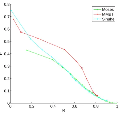
MMBT and MosesFigure 4.9 is a plot of R as a function of P for MMBT, Moses and Sinuhe.
We note that for the same value of R Moses generally has lower P than MMBT. This means that to cover the same amount of words in the test sentences, more words have been retrieved from Moses’s phrase table, leading to a larger raw search space to construct the translation from. In this respect, we can say that Moses’s phrase table contains more alternatives than MMBT’s. Among these alternatives, some are probably clearly wrong candidates but others can be correct translations that would have been used in other contexts. The prediction of the words is in that sense less deterministic with Moses.
When the full phrase table is taken into account (right end of the curves) Moses reaches a much better coverage, close to full coverage (R = 0.99) while with MMBT one fifth of the sentences remains uncovered (R = 0.81). The value of P when the full phrase table is taken into account is 6 × 10⁻²
1 1.5 2 2.5 3 3.5 0 0.1 0.2 0.3 0.4 0.5 0.6 0.7 0.8 0.9
Biphrases score threshold P R (a) MMBT (score=mmbt2/mmbt1) −0.2 0 0.2 0.4 0.6 0.8 1 1.2 0 0.1 0.2 0.3 0.4 0.5 0.6 0.7 0.8 0.9 1
Biphrases score threshold P
R
(b) Moses (score=mos1.mos3)
Figure 4.10: MMBT and Moses phrase tables coverage comparison over 100 test sentences, including biphrases with decreasing scores, P and R vs. thresholds
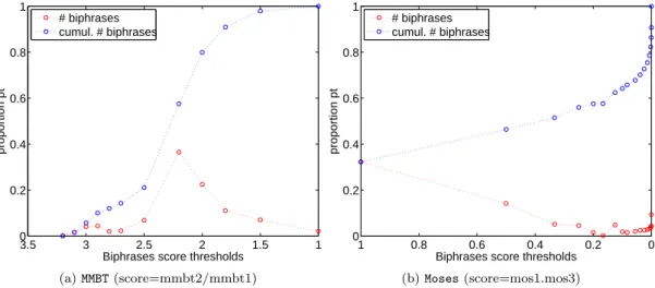
1 1.5 2 2.5 3 3.5 0 0.2 0.4 0.6 0.8 1 proportion pt
Biphrases score thresholds # biphrases cumul. # biphrases (a) MMBT (score=mmbt2/mmbt1) 0 0.2 0.4 0.6 0.8 1 0 0.2 0.4 0.6 0.8 1 proportion pt
Biphrases score thresholds # biphrases
cumul. # biphrases
(b) Moses (score=mos1.mos3)
Figure 4.11: MMBT and Moses biphrases distribution depending on their scores
Coverage and biphrases distribution
The evolution of R and P when more and more biphrases are included, aggregating words from phrases with decreasing scores, for MMBT and Moses, is shown on Figure 4.10a and Figure 4.10b respectively.
We can see that the increase of R is directly linked to the decrease of P . Increasing the coverage (as measured by R) is obtained by lowering the threshold to take in more biphrases, therefore building a larger bag of words, loosing precision (as measured by P ). The gain in coverage always remains proportional to the loss in precision.
The slope of the curve is mainly caused by the size of the portions of the phrase table that are aggregated when lowering the threshold on the score. We tried to use a score and thresholds set in order to cut the phrase table in equally sized portions to cut out this effect, but some large portions of the phrase table may have the same score and thus cannot be discriminated. The best example is the set of Moses’s biphrases scoring 1 which represent about a third of that phrase table.
de-0 0.2 0.4 0.6 0.8 1 0 0.2 0.4 0.6 0.8 1 P R sinuhe once words twenty tail
Figure 4.12: Sinuhe phrase table coverage comparison over 100 test sentences, including biphrases with decreasing scores, pruning using various methods, P vs. R
pending on their score shown on Figure 4.11a is very similar to the R curve of Figure 4.10b. Different scoring methods and threshold sets have been tried but we could not identify any subset of biphrases for which R and P were atypically related.
With MMBT, the R curve has a sharp increase for scores between 3 and 2.5, while the cumulative distribution of the biphrases (Figure 4.11a) does not show an equally sharp growth in the total number of biphrases between thoses scores but a rather small bump corresponding to the cluster with slope a1 = 2.886 mentioned in 4.2.3. Among a rather small number of biphrases from that
cluster, many have been retrieved and allowed to cover a significant part of the test sentences. This might indicate that this cluster contains biphrases of better quality.
Phrase table pruning
Next we look at how pruning the phrase table according to Sinuhe criteria affects the coverage. We used the score formula sin1
sin2.sin3. It corresponds directly to mos1.mos3, the formula used in the
previous section, allowing us to compare the results obtained with Moses’s phrase table and those obtained with Sinuhe’s.
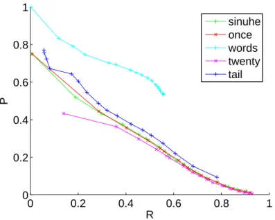
Figure 4.12 is a plot of R as a function of P for Sinuhe’s phrase table. The curve denoted sinuhe was obtained after applying the pruning used in Sinuhe described in 3.2.1, it was the same as the corresponding curve in Figure 4.9. The curve denoted once was obtained when applying the pruning used in Sinuhe but relaxing the pruning criterion on single co-occurrence of the pair (source phrase, target phrase) to a single occurrence of both source phrase and target phrase separately. Using only biphrases of length one on both sides restricting to the highest ranking candidate for each source phrase, i.e., using only word to word translation with the first candidate, we obtained the curve denoted as words. The curve denoted twenty was generated by removing only candidates ranked lower than twenty and the one denoted tail with multiple occurring biphrases, cutting the tail of candidates in a somewhat more elaborate way that we will detail later.
The values obtained for P and R for the different pruning methods when including the whole pruned phrase table (this corresponds to the rightmost point of each curve) are reported in Table 4.4.
The fact that using word to word matching with the best candidate (words) only allows to cover about half of the test data is an argument for using phrases with multiple candidates. Relaxing
pruning P R sinuhe 0.0207 0.9038 once 0.0120 0.9210 words 0.5358 0.5583 twenty 0.0065 0.9294 tail 0.0941 0.7813
Table 4.4: P and R for different pruning methods
the pruning criterion of one occurrence of the biphrase to one occurrence of both the source phrase and the target phrase (once) does not lead to a significant improvement over the original pruning when only multiple occurring biphrases ar kept (sinuhe). Only a little increase in coverage R at the expense of a smaller P , i.e., of a larger search space. Including all biphrases but still cutting the tail of candidates at the twentieth (twenty) has about the same effect, the coverage still increases by a few hundredth parts and the search space becomes still larger. This means that adding once occurring biphrases only brings few new useful terms but makes the search space larger, about twice as many distinct words to select the translation from in twenty as in sinuhe. Therefore, the decoding process might be slown down significantly only for little gain in translation quality. The last pruning technique, including only multiple occurring biphrases and cutting the tail of candidates depending on its shape allows to reach equivalent coverages with smaller search space than the three methods with fixed number of candidates. On the other hand its maximum coverage is only 0.78, letting a rather large fraction of data uncovered, and might be harmful to the translation quality.
Low rank biphrases
When using the complete phrase table, the value for R is very close to 1 for Moses, i.e., almost perfect recall is reached. In fact, this result appears to be misleading. We run the same coverage test, this time using only biphrases ranked further than the twentieth for a given source phrase. That phrase table contains only 11708 very frequent source phrases. Each of them is associated with a number of possible candidates. For example, the french word de is associated to 42569 different target phrases, pour to 11885 and pour les to 1713. In fact, almost all relatively common words from the target vocabulary have been extracted in some low ranking candidate. Since thoses source phrases are very frequent, several of them typically occur in each of the sentences to be translated. Then, almost all relatively common words are included in our target word bag and those that do occur in the target sentence can be found there even though they might have been generated only by chance from a distant word of the source sentence. This is how only rare words are left untranslated, yielding an almost perfect coverage, which is in fact only virtual, since as we explained it is generated merely by chance and cannot be handled by the decoder.
The number of candidates taken into account in the decoding process with Moses is generally limited to twenty, but the ranking of the candidates is not established on the same criteria. The values obtained for twenty (P = 0.0065, R = 0.9294), when removing only the low rank biphrases, therefore give a more accurate estimate of the operative setting also for Moses, even if it does not exactly correspond to the restriction applied on the search beam during the decoding process.
4.5 Tail cutting, translation quality and speed
Some phrases have a very large number of candidate translations, as we pointed out in the preceding section. Some among these candidates are erroneous translations, others are more or less literal translations. In this section we concentrate on the question of how many candidates to keep for each phrase.
Figure 4.13: Partition of Sinuhe biphrases depending on their occurrence counts
4.5.1 Sinuhe pruning
Out of the 46.4 million biphrases of the original phrase table, about a third (14.9 MB) contains an unaligned end word (Figure 4.13). About another third is made up by biphrases that occur once and whose source phrase and target phrase occur once. These biphrases are denoted by their characteristic 1-1-1 occurrence count. Almost all of the last third of the phrase table is composed of once occurring biphrases for which either the source phrase, the target phrase or both occur more than once. This group of biphrases will later be referred to as unique biphrases. The remaining multiple occurring biphrases represent only about 5% of the original phrase table. The original prunig method for Sinuhe keeps only the last group of biphrases.
An additional criterion for filtering the biphrases is one based on their rank. The biphrases that share the same source phrase are ranked in decreasing order of occurrence count and only those ranked over k are kept, where k is a parameter than can be modified in the configuration and is typically set to twenty. Note that since some biphrases can occur the same number of time there can be several biphrases having the same rank. In this case, if for example three biphrases have equal rank four, there won’t be any biphrase with rank five or six and the next biphrase will have rank seven. For that reason, phrases with more than twenty multiple occurring biphrases may not have exactly twenty candidates after pruning.
Furthermore, the ranking is established before any pruning. The once occurring biphrases do not have an influence on the ranking since they would always be ranked last. On the other hand, since the ranking is done before filtering out unaligned biphrases, some of them may be ranked among the twenty most frequent candidates, leaving holes in the ranking when they are removed. As an example, the tails of candidates of two source phrases are given as the sequence of the counts of occurrence of the candidate biphrases in decreasing order of occurrence. The subscripts indicates the rank and unaligned biphrases are displayed between parenthesis.
devions: 781 602 503 424 295 236 127 118 99 99 711 612 612 514 315 315 315 315 219 219 219 219
219 (2)19(2)19 (2)19. . .
de mani`ere `a: (108)1852843(82)4(54)5(51)6497408369(35)102711(26)122513(23)14(19)15
1816 1617 (16)17 (15)19 (15)19 1421 (13)22 (13)22 1224 1224 1224 (11)27 (11)27 (11)27 930 930 832
(8)32(7)34 (7)34 (7)34(6)37(6)37 (6)37 (6)37541 (5)41(5)41 (5)41 (5)41. . .
The first case shows how more than twenty candidates can be kept for the same source phrase. After pruning, the source phrases devions will have 23 candidates. The second case is an extreme example of how frequent unaligned biphrases can lead to a short tail of candidates after pruning. The source phrase de mani`ere `a will only have 9 candidates after pruning.
A similar fixed rank tail cutting also happens in Moses since the number of candidates for a given input phrase is limited during the decoding. This parameter is defined in the configuration file and is typically set to twenty.